FPGA-Based Dual Learning Model for Wheel Speed Sensor Fault Detection in ABS Systems Using HIL Simulations

Abstract

The rapid evolution of modern vehicles into intelligent and interconnected systems presents new complexities in both functional safety and cybersecurity. In this context, ensuring the reliability and integrity of critical sensor data, such as wheel speed inputs for anti-lock brake systems (ABS), is essential. Effective detection of wheel speed sensor faults not only improves functional safety, but also plays a vital role in keeping system resilience against potential cyber–physical threats. Although data-driven approaches have gained popularity for system development due to their ability to extract meaningful patterns from historical data, a major limitation is the lack of diverse and representative faulty datasets. This study proposes a novel dual learning model, based on Temporal Convolutional Networks (TCN), designed to accurately distinguish between normal and faulty wheel speed sensor behavior within a hardware-in-the-loop (HIL) simulation platform implemented on an FPGA. To address dataset limitations, a TruckSim–MATLAB/Simulink co-simulation environment is used to generate realistic datasets under normal operation and eight representative fault scenarios, yielding up to 5000 labeled sequences (balanced between normal and faulty behaviors) at a sampling rate of 60 Hz. Two TCN models are trained independently to learn normal and faulty dynamics, and fault decisions are made by comparing the reconstruction errors (MSE and MAE) of both models, thus avoiding manually tuned thresholds. On a test set of 1000 sequences (500 normal and 500 faulty) from the 5000 sample configuration, the proposed dual TCN framework achieves a detection accuracy of 97.8%, a precision of 96.5%, a recall of 98.2%, and an F1-score of 97.3%, outperforming a single TCN baseline, which achieves 91.4% accuracy and an 88.9% F1-score. The complete dual TCN architecture is implemented on a Xilinx ZCU102 FPGA evaluation kit (AMD, Santa Clara, CA, USA), while supporting real-time inference in the HIL loop. These results demonstrate that the proposed approach provides accurate, low-latency fault detection suitable for safety-critical ABS applications and contributes to improving both functional safety and cyber-resilience of braking systems.

1. Introduction

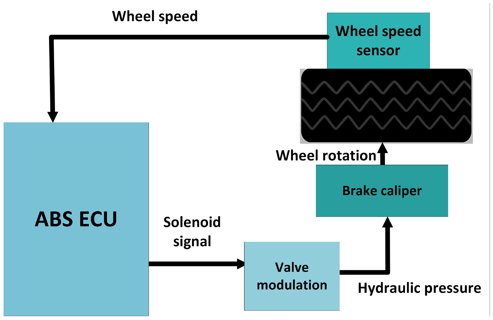
Modern vehicles integrate hundreds of electronic control units (ECUs) coordinating safety-critical functions such as braking, steering, and powertrain control [1]. As system complexity grows, so does the risk of component failures that can compromise vehicle safety. Among these, the anti-lock braking system (ABS) ECU plays a critical role in preventing wheel lockup during emergency braking, ensuring vehicle stability and steerability [2]. Wheel speed sensors provide essential input data to the ABS ECU; their failure or malfunction can lead to loss of braking effectiveness and steering control.

Detecting sensor faults in real time presents significant challenges. Traditional fault detection methods rely on manually defined thresholds and expert knowledge, making them time-consuming to develop and difficult to adapt to diverse operating conditions [3]. Furthermore, acquiring representative faulty sensor data for validation is problematic, as generating real faults in safety-critical systems is both risky and expensive [4]. Hardware-in-the-loop (HIL) simulation offers a controlled testing environment, but existing HIL-based fault detection approaches struggle with real-time performance requirements and adaptive fault classification [5,6].

Recent advances in deep learning, particularly Temporal Convolutional Networks (TCNs), have demonstrated superior performance in modeling sequential sensor data compared to recurrent architectures [7]. However, deploying these models on conventional computing platforms (CPUs/GPUs) introduces latency and power consumption incompatible with automotive real-time constraints. Field-Programmable Gate Arrays (FPGAs) provide an alternative, offering deterministic low-latency execution with significantly higher energy efficiency than GPUs [8].

This paper addresses these challenges by proposing a novel dual-learning framework based on TCNs for wheel speed sensor fault detection in ABS systems, implemented on FPGA hardware for real-time operation within HIL simulation platforms. Unlike conventional single-model approaches that learn only normal behavior, our dual-TCN architecture explicitly learns both normal and faulty sensor patterns, enabling threshold-free fault classification through comparative error analysis.

Main Contributions:

• A novel dual-learning TCN framework that simultaneously models normal and faulty wheel speed sensor behaviors, achieving 97.8% classification accuracy without manual threshold tuning.
• Real-time FPGA implementation enabling proactive fault detection before corrupted data reaches the ABS ECU.
• A systematic co-simulation methodology using MATLAB/Simulink and TruckSim (v2020.X, Mechanical Simulation Corporation, Ann Arbor, MI, USA) to generate eight representative fault scenarios, addressing the challenge of acquiring realistic faulty sensor datasets.
• Comprehensive validation on a HIL platform with a commercial Bendix EC-60 ABS ECU (Bendix Commercial Vehicle Systems LLC, Avon, OH, USA), demonstrating practical applicability to safety-critical automotive systems.
• An extensible dual-TCN monitoring block that can be retrained and reused for other safety-critical ECUs and sensor-driven subsystems, enabled by its modest FPGA resource footprint and generic sequence-modeling design.

In this study, normal behavior refers to the wheel speed sensor operation under fault-free conditions, whereas abnormal behavior denotes sensor behavior in the presence of injected faults.

The remainder of this paper is organized as follows. Section 1 reviews related work on HIL-based ECU validation, data-driven fault diagnosis, and ABS sensor fault detection. Section 2 presents the ABS system model. Section 3 describes the proposed methodology, including data generation, dual-TCN architecture, and FPGA implementation. Section 4 details the experimental setup and HIL platform. Section 5 reports and discusses the experimental results. Finally, Section 6 concludes the paper.

2. Related Work

HIL simulation has become a standard tool for validating automotive ECUs under realistic but safe conditions [5,6]. In such platforms, real-time vehicle dynamics models are coupled with physical ECUs to reproduce road scenarios, driver inputs, and component faults. As HIL-based real-time simulation for embedded control development and automated testing has matured, increasing attention has been devoted to analyzing how complex embedded ECU control software (i.e., firmware/control logic) behaves under abnormal or faulted operating conditions. For instance, Poon et al. [9] demonstrated that an HIL platform with fault injection can be used to systematically evaluate electric vehicle drive systems. Similarly, Abboush et al. [10] implemented a real-time fault-injection framework on a MATLAB/Simulink-based HIL bench with a prototype ECU, where multiple classes of sensor and actuator faults are injected in software without modifying the plant model. In contrast, our work uses the HIL bench to host a learned dual-model monitor that distinguishes normal and faulty wheel-speed behavior online, providing continuous sensor health assessment rather than exhaustive fault-injection coverage.

Within braking systems, ABS ECUs are especially sensitive to the quality of wheel speed sensor signals, since inaccurate speed measurements directly affect braking performance and vehicle stability [2]. Prior work on ABS fault detection has explored model-based observers, heuristic rules, and data-driven classifiers to detect wheel lock, slip, or sensor malfunctions [2,4,11]. While these approaches can successfully identify certain fault types, they often focus either on high-level ABS performance or on specific failure patterns, and typically assume that faulty data can be collected directly on test vehicles [12]. The safety and practical challenges of generating diverse faults in real vehicles motivate the use of simulation-based data generation; however, only a limited number of studies exploit high-fidelity co-simulation tools such as TruckSim for systematic modeling of wheel speed sensor faults.

In parallel, advances in computing and storage have accelerated the adoption of data-driven methods for fault diagnosis [13]. Deep neural networks—such as autoencoders (AEs and DAEs), convolutional neural networks (CNNs), recurrent neural networks (RNNs), and temporal convolutional networks (TCNs)—have been successfully applied to detect and classify faults in industrial and automotive systems [14,15,16]. These models can automatically extract hierarchical features from raw signals and frequently outperform traditional model-based approaches. Nevertheless, many reported solutions assume the availability of large labeled datasets, suffer from imbalanced or scarce faulty samples [14], or follow a single-model anomaly-detection paradigm in which a network learns only normal behavior and a fixed reconstruction- or anomaly-score threshold is used to declare faults [17,18].

Recent work has applied such deep learning techniques to a range of safety-critical domains [19,20,21,22,23]. For automotive HIL testing, Abboush et al. [19] proposed a hybrid CNN–LSTM network deployed on a PC-based HIL bench to classify eight injected sensor and actuator faults in a gasoline engine ECU, reporting approximately 98.8% accuracy, precision, recall, and F1-score over nine classes. In contrast, the present work targets ABS wheel-speed sensors and integrates the fault-detection model directly into the HIL loop as an FPGA-resident accelerator, enabling deterministic real-time operation with low latency.

Beyond automotive systems, several authors have employed LSTMs, CNNs, and TCNs for fault diagnosis in other cyber–physical systems. Malhotra et al. [22] used LSTM networks for anomaly detection in spacecraft telemetry, training a single model on normal data and identifying faults via an anomaly-score threshold, achieving an anomaly recall of about 89%. Guo et al. [23] proposed a hierarchical adaptive CNN for bearing fault diagnosis and reported classification accuracies around 99% over ten fault classes. Fang et al. [20] combined an enhanced TCN with a meta-heuristic optimizer for nuclear power plant fault diagnosis, obtaining higher accuracy than conventional deep learning baselines. Similarly, Cummins et al. [21] used a TCN as a normal-only anomaly detector for bearing condition monitoring and augmented it with counterfactual explanations for what-if analysis. All of these methods instantiate the single-model paradigm described above, either directly classifying fault types with a single network or declaring anomalies via a tuned threshold on a normal-trained model.

Deploying deep learning models in real-time automotive environments also raises hardware constraints. GPUs, although powerful, are usually unsuitable for embedded ECUs due to power, cost, and integration limitations. FPGAs have therefore attracted increasing interest as neural network accelerators, offering an order-of-magnitude improvement in energy and delay efficiency compared with GPUs [8]. Several works report FPGA-based implementations of CNNs and RNNs for generic time-series processing, yet there is little research on FPGA-accelerated TCNs tailored to automotive HIL fault detection. Even fewer examples integrate such accelerators into a closed-loop HIL platform that interacts with a commercial ABS ECU.

Taken together, the existing literature reveals three main gaps. First, most HIL studies do not embed a dedicated, learning-based sensor health monitoring module directly within the HIL loop. Second, deep learning approaches for fault detection commonly rely on single-model architectures that require manual threshold tuning or do not explicitly model faulty behavior, which can reduce robustness across heterogeneous fault modes. Third, there is limited reported work on FPGA-based deployment of dual-learning models (normal vs. faulty) for real-time ABS sensor fault detection using realistic, simulation-derived datasets. The framework proposed in this paper addresses these gaps by: (i) integrating a dual-TCN sensor fault detection module into an ABS HIL platform; (ii) explicitly learning normal and faulty behavior through two complementary TCN models and using their comparative reconstruction errors as an implicit decision rule, thereby eliminating the need for manually tuned thresholds required by single-model schemes; and (iii) implementing the complete architecture on a Xilinx ZCU102 FPGA, demonstrating both high detection performance and feasibility for real-time embedded deployment.

Table 1. Position of the proposed dual-TCN approach with respect to representative deep learning-based fault diagnosis methods.

Ref.	Domain & Target	Core Model	Learning Scheme	Deployment	Key Performance	Key Limitation/ Characteristic
[22]	Automotive HIL (engine ECU)	CNN–LSTM	Supervised classification	PC/HIL	≈98.8% accuracy (9 classes)	PC-based; not integrated as a deterministic in-loop monitor
[22]	Spacecraft telemetry	LSTM	Single (normal-only anomaly detection)	GPU	≈89% anomaly recall	Threshold-dependent; models only normal behaviour
[23]	Bearing diagnostics	CNN	Single (multi-class fault classification)	GPU	≈99% accuracy (10 fault classes)	Offline GPU-based analysis; no HIL or ECU integration
[20]	Nuclear power plant CPS	Enhanced TCN	Supervised classification	PC	Higher accuracy than DL baselines	Domain-specific; PC-based simulation environment
This work	Automotive HIL (ABS ECU, wheel-speed sensors)	Dual TCN	Dual-model comparative (normal vs. faulty)	FPGA (ZCU102)	97.8% accuracy, 97.3% F1-score	Threshold-free; deterministic real-time FPGA in-loop monitor

summarizes the position of the proposed framework relative to these representative methods in terms of target system, model type, learning scheme, deployment platform, and reported performance. Compared to this state of the art, our work introduces three complementary contributions: (i) a dual-learning TCN architecture that explicitly models both normal and faulty wheel-speed behavior and performs threshold-free discrimination via comparative reconstruction errors; (ii) a complete HIL-based workflow, from TruckSim/Simulink fault-scenario generation to closed-loop interaction with a commercial Bendix EC-60 ABS ECU; and (iii) an FPGA implementation that achieves 97.8% accuracy and a 97.3% F1-score on eight representative fault scenarios while using only 12.7% of LUTs, 19.1% of BRAMs, and 5.1% of DSP slices on a ZCU102 evaluation board (AMD, Santa Clara, CA, USA). This combination of dual learning, HIL integration, and resource-efficient FPGA deployment is, to the best of our knowledge, not jointly addressed in prior work.

3. ABS System Model

The ABS is a critical safety feature in modern vehicles designed to prevent wheel lock-up and maintain steering control during abrupt braking maneuvers. A standard four-wheel ABS configuration, illustrated in Figure 1, consists of wheel speed sensors, an ECU, a hydraulic modulator, and solenoid valves [24].

The ABS functions as a closed-loop control system. The wheel speed ${\omega }_w$ is continuously measured by the sensors and transmitted to the ECU. Using this information, the ECU computes the wheel slip ratio $\lambda$, a key variable that determines whether the wheel is approaching lock-up:

$$\lambda ={\displaystyle \frac{v-r_w{\omega }_w}{v}},$$

(1)

where v denotes the vehicle velocity and $r_w$ represents the effective wheel radius. When the slip ratio $\lambda$ exceeds a predefined limit ${\lambda }_{max}$, the ECU issues control commands to the hydraulic modulator to regulate the brake pressure applied to the wheel cylinder.

The rotational dynamics of the wheel can be expressed as:

$$J_w{\displaystyle \frac{d{\omega }_w}{dt}}=T_b-r_w{F}_x,$$

(2)

where $J_w$ is the wheel’s moment of inertia, $T_b$ is the brake torque, and $F_x$ is the longitudinal tire–road interaction force. The brake torque is dynamically adjusted by the ECU through a feedback controller, typically implemented in a PID structure:

$$T_b\left(t\right)=K_{p}e\left(t\right)+K_i{\int }_0^{t}e\left(\tau \right)d\tau +K_d{\displaystyle \frac{de\left(t\right)}{dt}},e\left(t\right)={\lambda }_{\mathrm{target}}-\lambda \left(t\right).$$

(3)

This closed-loop operation enables real-time adjustment of braking pressure to maintain the desired slip ratio, thereby optimizing braking performance while preserving vehicle stability and steering control [25].

4. Methodology

The proposed methodology introduces an FPGA-based proactive framework for early sensor-level fault detection, thereby enhancing the reliability and safety of the ABS ECU. Unlike conventional approaches that rely solely on the ECU for anomaly detection, the proposed system monitors and analyzes wheel speed sensor data before it reaches the ECU, preventing the transmission of corrupted signals that could adversely affect braking performance.

The methodology is centered on a dual-learning framework employing TCNs. Two distinct TCN models are trained: one to represent normal sensor behavior and the other to represent faulty behavior. Each model predicts the expected wheel speed signal sequence based on its respective learned dynamics. The reconstruction errors between the predicted and observed signals are computed using both the Mean Squared Error (MSE) and the Mean Absolute Error (MAE). A decision logic block then compares these errors to classify the incoming signal as either normal or faulty.

To eliminate reliance on manually defined fault thresholds and enhance detection robustness, the proposed framework adopts a comparative decision strategy that uses two TCN models rather than a single model. During evaluation, an input sequence is simultaneously processed by both networks, and their reconstruction performance is assessed through the aforementioned error metrics. The framework determines which model better explains the observed signal: when the errors corresponding to the faulty-trained model are smaller than those of the normal-trained model, the input is classified as faulty; conversely, if the normal-trained model yields smaller errors, the input is identified as normal. This comparative approach removes the need for predefined thresholds and provides a more adaptive and robust mechanism for fault detection.

Unlike single-TCN approaches that rely on a fixed MSE threshold to discriminate between normal and abnormal conditions, the dual-model configuration enables a direct comparison between two learned behavioral spaces. This design inherently compensates for environmental variability, signal scaling, and sensor noise, thereby making the classification process more adaptive and data-driven. Furthermore, while a single model primarily learns nominal dynamics and flags large deviations as faults, the dual-TCN architecture explicitly captures the statistical and temporal characteristics of both healthy and faulty states. Consequently, it can detect subtle or early sensor-level deviations that may fall below fixed threshold limits, offering improved sensitivity, reduced false alarms, and enhanced robustness across diverse operational and fault scenarios.

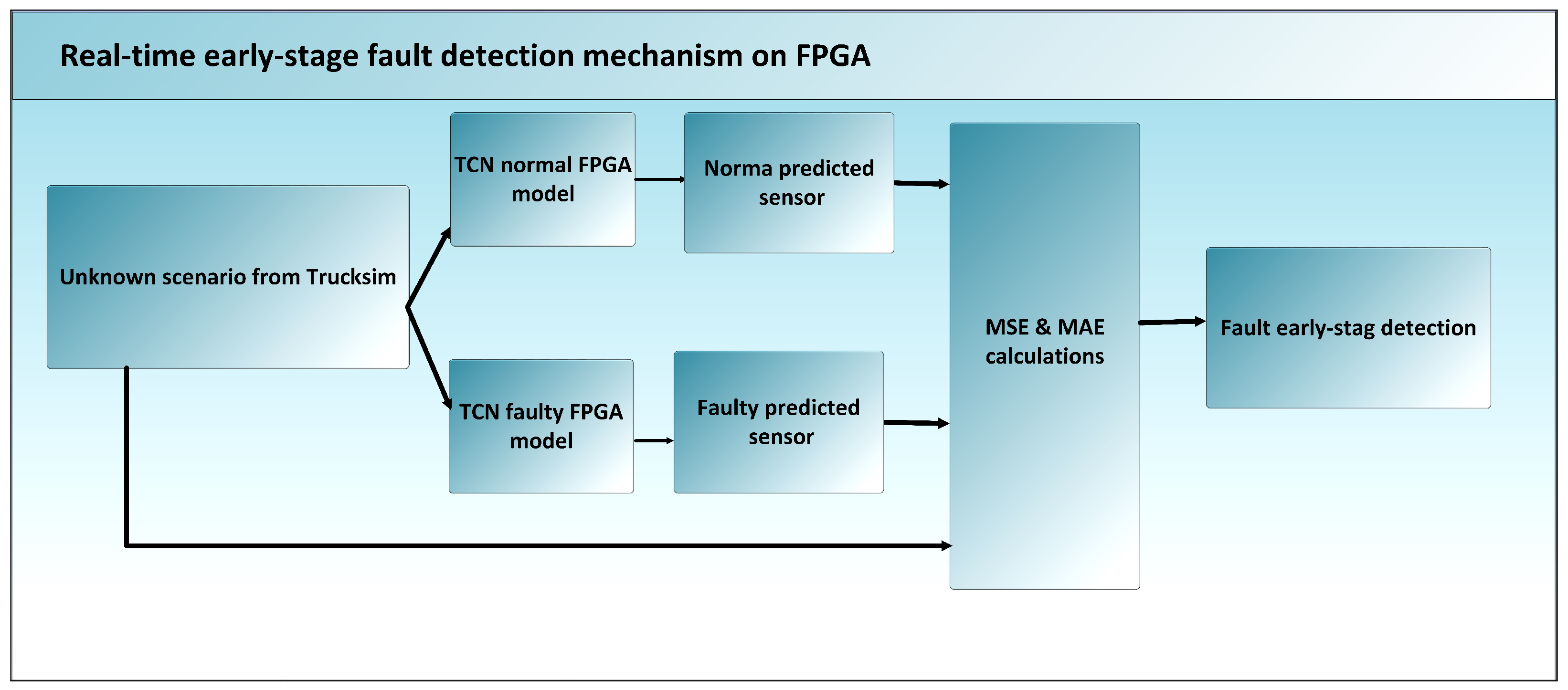
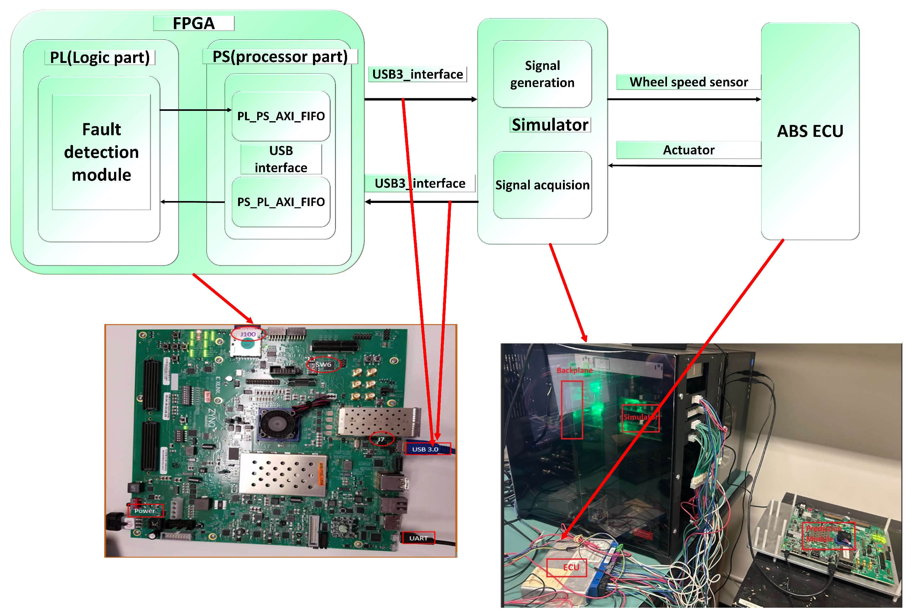
For real-time deployment, the proposed fault detection mechanism is implemented on an FPGA, as illustrated in Figure 2. It integrates TruckSim as the vehicle dynamics simulator to provide wheel speed data under various faulty and normal driving scenarios. These sensor signals are transmitted in real time to the FPGA-based fault detection module.

As shown in the figure, the incoming wheel speed data from TruckSim are simultaneously applied to two TCN models deployed on the FPGA: the TCN-normal FPGA model and the TCN-faulty FPGA model. Each model predicts how the corresponding wheel speed sensor should behave—one based on learned normal dynamics and the other based on faulty behavior. The outputs of the two models, referred to as the normal predicted sensor and the faulty predicted sensor, are forwarded to the MSE and MAE calculation block. This block computes and compares the reconstruction errors of both predictions relative to the TruckSim reference signal.

The comparative error analysis enables the system to identify the model that better represents the observed sensor behavior. When the faulty model exhibits lower errors, the input is classified as faulty; otherwise, it is considered normal. The final classification result is generated by the fault detection block, completing the real-time early sensor-level fault detection.

Overall, the FPGA-based HIL framework operates as a low-latency, parallel inference system capable of evaluating wheel speed sensor health directly from TruckSim scenarios. By performing MSE and MAE comparison between two behavior-specific TCN models, the architecture achieves proactive and threshold-free fault detection for ABS applications.

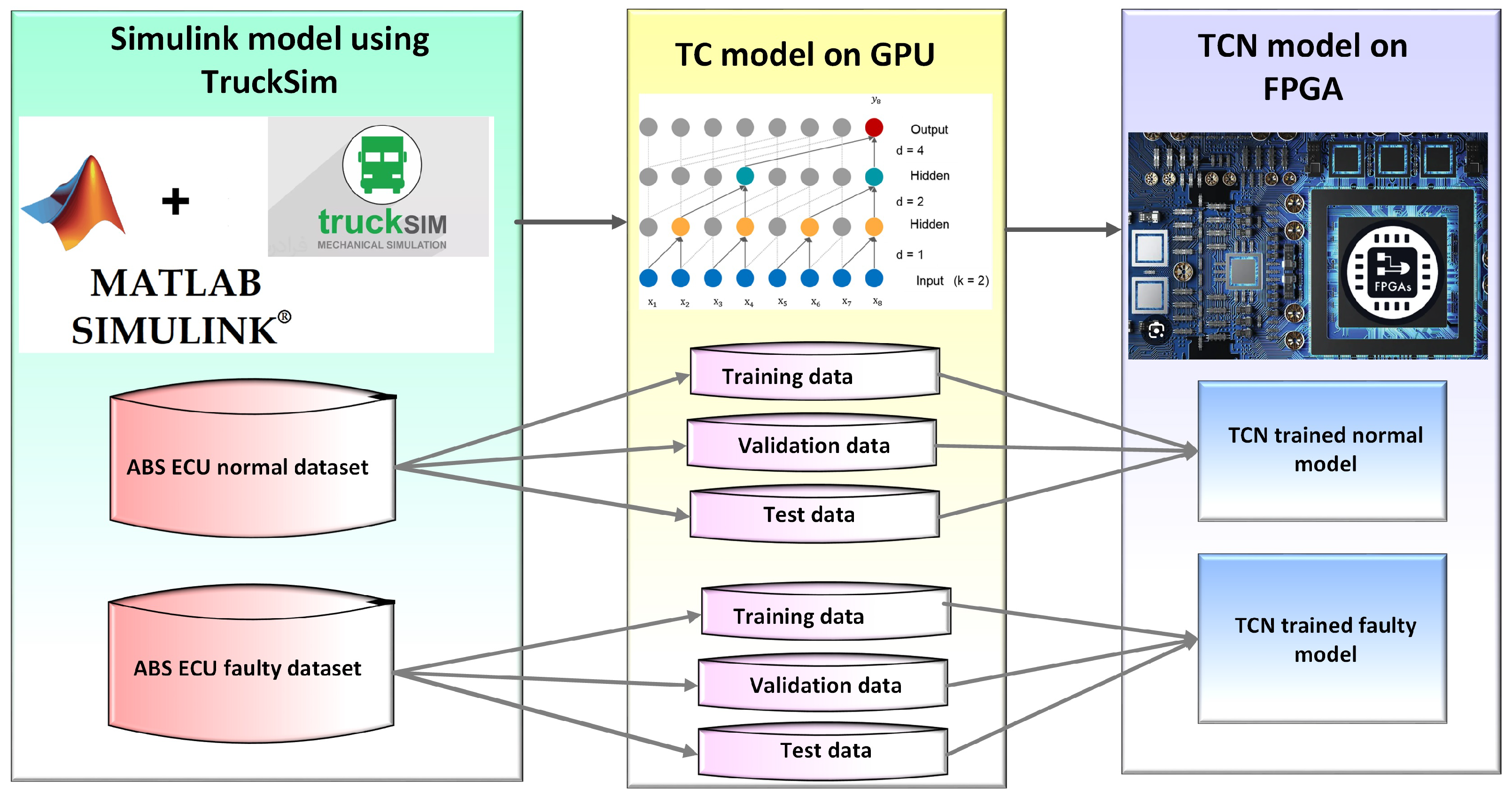
The proposed FPGA-based fault detection mechanism is organized into three main components: data augmentation, dual-model feature learning, and FPGA-based classifier deployment, as illustrated in Figure 3.

In the first stage, data augmentation is performed through a co-simulation framework that integrates TruckSim with MATLAB/Simulink. Various driving conditions (including changes in vehicle speed, braking pressure, and steering angle) are simulated to generate comprehensive datasets for both normal and faulty ABS ECU operation. Normal datasets capture healthy wheel speed sensor behavior, while faulty datasets are created by introducing fault patterns into the sensor models. This approach ensures diverse and realistic training samples for both operational states.

In the second stage, dual-model feature learning is carried out using TCNs trained on a GPU. The augmented datasets are partitioned into training, validation, and testing subsets. Two independent TCNs are then trained: one exclusively on normal data and the other on faulty data. Each model learns the temporal dependencies and statistical signatures characteristic of its respective condition, establishing two distinct behavioral representations.

In the final stage, both trained TCN models are deployed on FPGA hardware for real-time inference and classification. The FPGA executes the models in parallel, processing live wheel speed signals and comparing the prediction errors (measured by the MSE and MAE) to determine the sensor’s health state. This real-time deployment enables proactive fault detection and low-latency fault response, enhancing the overall reliability and safety of the ABS.

4.1. Simulation Model

To train and evaluate the proposed framework, two comprehensive datasets (representing both normal and faulty operating conditions) were generated for ABS ECU fault detection. The integration of TruckSim with MATLAB/Simulink enables high-fidelity co-simulation of vehicle dynamics and fault scenarios by modifying input signals, parameters, and environmental conditions. Because the wheel speed sensor output depends directly on the vehicle’s longitudinal velocity, braking torque, and steering dynamics, faulty sensor behavior can be effectively emulated by altering these parameters in the simulation.

In this study, eight representative fault scenarios were systematically introduced in TruckSim by manipulating specific input parameters of TruckSim. These scenarios simulate realistic cases in which the ABS fails to operate correctly. The corresponding wheel speed sensor data were collected to form a diverse faulty dataset for model training and evaluation.

According to recent literature, faults in automotive ECUs are generally classified into hardware, software, and communication/network categories, depending on the affected subsystem [19]. The faults modeled in this work primarily correspond to hardware-type sensor faults, representing signal abnormalities that arise from degradation, calibration drift, or sensor malfunction.

A TruckSim Simulink model framework was developed to replicate the dynamic behavior of a heavy vehicle equipped with an ABS ECU. TruckSim provides a physics-based vehicle dynamics model, while Simulink handles signal generation, control logic, and fault injection using MATLAB function blocks. This combined setup allows realistic simulation of both nominal and faulty driving conditions, ensuring accurate and diverse data generation for the TCN-based fault detection model.

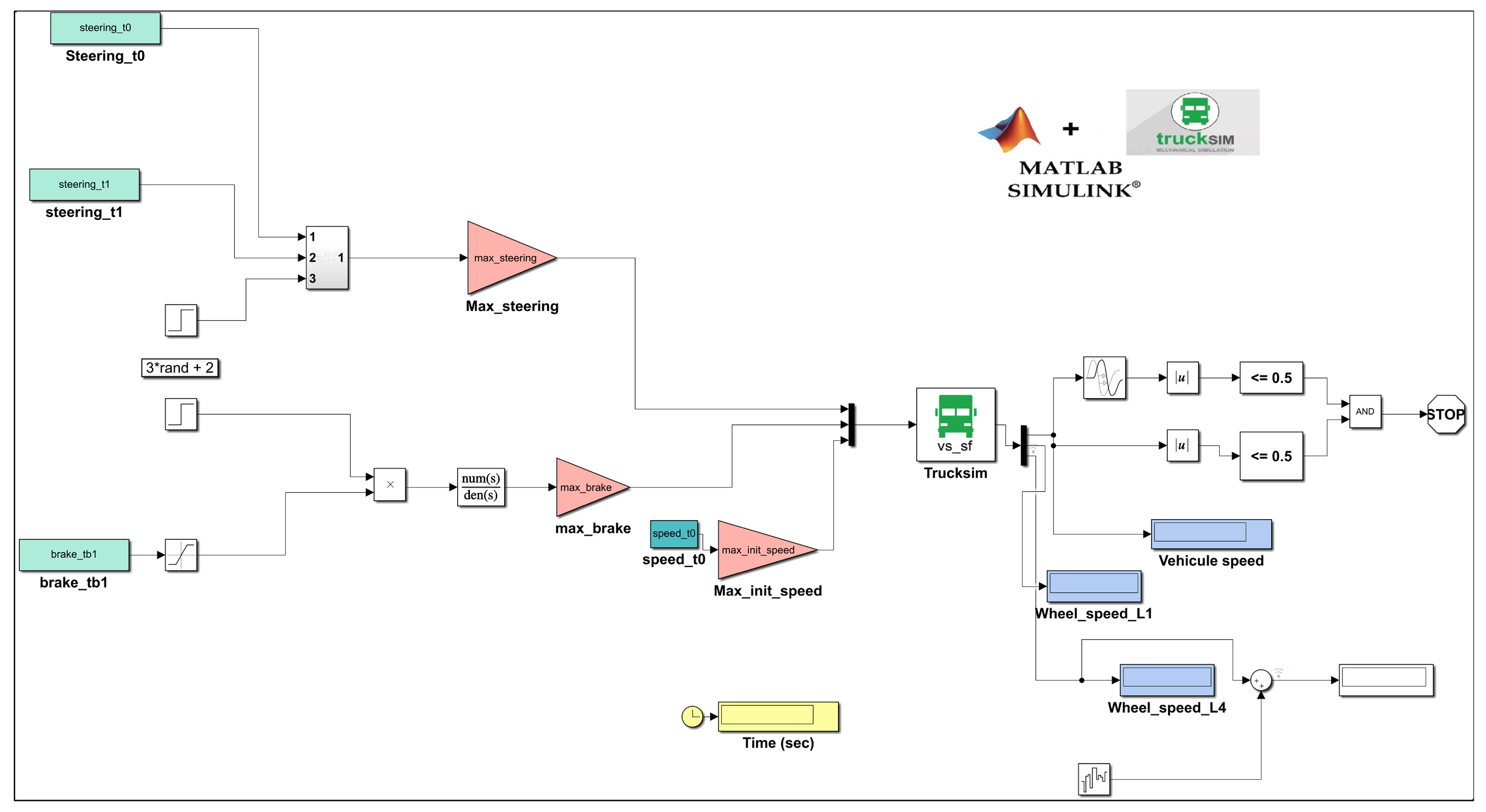
As shown in Figure 4, the left section of the model represents the input generation stage, where the steering angle, the braking torque, and the initial vehicle speed are defined using MATLAB function blocks and parameterized signal sources. These time-varying signals are transmitted to the TruckSim interface block to drive the vehicle model.

TruckSim then processes these control inputs to simulate realistic vehicle dynamics under varying operating conditions. The resulting outputs, such as vehicle speed, individual wheel speeds, yaw rate, and lateral acceleration, are fed back into Simulink for data logging, analysis, and fault evaluation. MATLAB functions thus serve as time-driven signal generators that map simulation time to dynamic driving behaviors, including steering oscillations, braking maneuvers, and velocity variations, ensuring diversity across all simulation runs.

The simulation utilizes two dedicated MATLAB function blocks that generate the steering wheel angle and brake pressure command as time-varying inputs to TruckSim. These signals define the driving maneuvers and braking behavior of the vehicle, enabling the analysis of ABS performance under diverse road conditions.

To simulate realistic driver behavior, steering and braking inputs are generated using random processes with truncated normal and uniform distributions. For example, the initial vehicle speed $v_{t0}$ is sampled as $v_{t0}\sim \mathcal{N}({\mu }_v=0.67,{\sigma }_v^2=0.{56}^2)$, truncated to $[0.17,1]$, to ensure that the sampled values correspond to the physical speed range of $[20,120]$ km/h while maintaining a realistic spread around the typical driving speed. The limits are derived from $v_{max}=120\mathrm{km}/\mathrm{h}$, $v_{min}=20\mathrm{km}/\mathrm{h}$, and $v_{\mathrm{range}}=100\mathrm{km}/\mathrm{h}$, resulting in:

$${\mu }_v={\displaystyle \frac{v_{\mathrm{range}}/2+v_{min}+10}{v_{max}}}=0.67,{\sigma }_v={\displaystyle \frac{v_{\mathrm{range}}}{1.5v_{max}}}=0.56,[v_{min}/v_{max},1]=[0.17,1].$$

(4)

Similarly, the initial brake and steering commands are sampled as

$$b_{t0}(\mathrm{m}/{\mathrm{s}}^2)=\left\{\begin{array}{cc}0,\hfill & p=0.08,\hfill \\ \mathcal{N}({\mu }_b=0.14,{\sigma }_b^2=0.3^2),\hfill & p=0.92\hfill \end{array}\right.,$$

(5)

$${\delta }_{t0}{(}^{\circ })=\left\{\begin{array}{cc}0,\hfill & p=0.1,\hfill \\ \mathcal{N}\left(0,{({\delta }_{\max \_\mathrm{init}}/1.5)}^2\right),\hfill & p=0.9\hfill \end{array}\right.,$$

(6)

where

$${\delta }_{\max \_\mathrm{init}}={\displaystyle \frac{1.5(-1.7v_{t0}{v}_{max}+260)}{720}}.$$

(7)

Here, v denotes the vehicle speed (normalized by $v_{max}$, mapping $[0.17,1]$ to $[20,120]$ km/h); b denotes the brake command (longitudinal deceleration, in $\mathrm{m}/{\mathrm{s}}^2$); and $\delta$ denotes the steering angle (in degrees). $\mathcal{N}(\mu ,{\sigma }^2)$ represents a normal distribution, and p indicates the sampling probability. Values drawn from $\mathcal{N}$ are truncated to the specified interval.

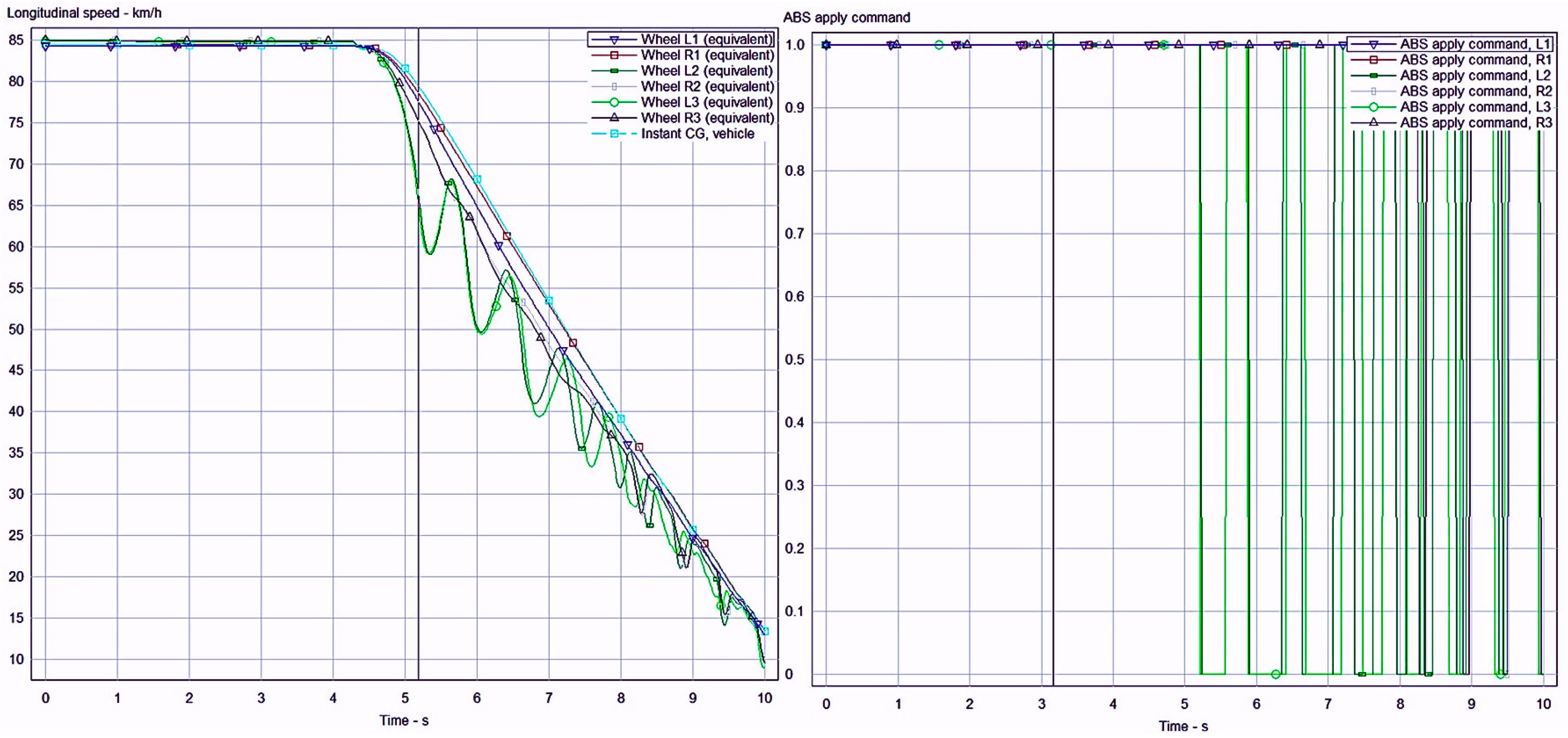
Normal behavior was obtained by simulating braking and steering events without any fault injection. The ABS ECU functioned correctly to prevent wheel lock while maintaining smooth deceleration. Figure 5 shows an example of normal braking behavior in TruckSim: the vehicle and wheel speeds decrease uniformly, while the ABS activation pattern remains stable and pulsed, indicating proper operation under nominal conditions.

4.2. Fault Scenario Modeling

To test the fault-detection capability of the proposed model, a range of fault scenarios was generated in the TruckSim–Simulink environment. These faults emulate actuator delays, sensor malfunctions, and abnormal driver inputs, which could degrade ABS performance or cause instability in the vehicle dynamics.

Table 2. Summary of normal and faulty scenarios generated in TruckSim–Simulink simulations.

Scenario	Affected Signals	Fault Type	Description and Effect
0	None	Normal	Vehicle dynamics follow normal steering, braking, and speed profiles.
1	Brake, Steering	Delay	Random delays added to brake (up to 0.5 s) and steering (up to 2 s) to simulate slow actuator response.
2	Brake	Delay	Brake actuation delayed randomly (up to 1 s) without affecting steering.
3	Wheel speed, Brake, Steering	Stuck-at value	Wheel speed sensor stuck at a constant value; brake and steering delayed to simulate sensor failure or control lag.
4	Brake	Sudden maximum	Vehicle initial speed is limited; brake torque set to maximum instantly to simulate emergency braking.
5	Wheel speed, Brake	Drift	Gradual increase in wheel speed and gradual decrease in braking torque over time to mimic sensor drift or calibration error.
6	Wheel speed	Spike or Drop	Random speed spike or sudden drop to test sensor fault or extreme dynamic event.
7	Wheel speed, Brake	Scaling error	Sensor outputs amplified or reduced, causing inconsistent speed and braking behavior.
8	Steering	Saturation	Steering input amplified up to maximum limits, simulating extreme or erroneous driver input.

summarizes the eight fault scenarios considered, including the affected signals, fault types, and their high-level impact on the system.

To provide a more formal mathematical definition suitable for discrete-time simulation, each fault scenario was implemented with its corresponding signal-level formulation.

Table 3. Fault scenarios in Simulink MATLAB model.

Fault Type	Fault Description	Discrete-Time Formulation	Effect on Vehicle Dynamics	Initial Values
1	Brake and steering delay	$b\left[n\right]=\left\{\begin{array}{cc}0,\hfill & n\mathrm{\Delta }t<{\tau }_b,\hfill \\ b_{\mathrm{t}0},\hfill & n\mathrm{\Delta }t\ge {\tau }_b,\hfill \end{array}\right.$ ${\tau }_b\in U[0,0.5]$ s $\delta \left[n\right]=\left\{\begin{array}{cc}0,\hfill & n\mathrm{\Delta }t<{\tau }_s,\hfill \\ {\delta }_{\mathrm{t}0},\hfill & n\mathrm{\Delta }t\ge {\tau }_s,\hfill \end{array}\right.$ ${\tau }_s\in U[0,2]$ s	Braking and steering responses are delayed, making vehicle control harder	Speed: $v_{t0}$ (km/h) $\sim N({\mu }_v=0.67,{\sigma }_v^2=0.{56}^2)$, truncated to $[0.17,1]$. Equivalent to $v_{t0}\in [20,120]$ km/h. ${\mu }_v={\displaystyle \frac{v_{\mathrm{range}}/2+v_{min}+10}{v_{max}}}=0.67$, ${\sigma }_v={\displaystyle \frac{v_{\mathrm{range}}}{1.5v_{max}}}=0.56$. $[v_{min}/v_{max},1]=[0.17,1]$, $v_{max}=120$ km/h, $v_{min}=20$ km/h, $v_{\mathrm{range}}=100$ km/h.   Brake: $b_{t0}$ (m/s2) $=\left\{\begin{array}{cc}0,\hfill & p=0.08,\hfill \\ N({\mu }_b=0.14,{\sigma }_b^2=0.3^2),\hfill & p=0.92\hfill \end{array}\right.$ Truncated to $[0,1]$.   Steering: ${\delta }_{max,\mathrm{init}}{(}^{\circ })={\displaystyle \frac{1.5(-1.7v_{t0}{v}_{max}+260)}{720}}$. ${\delta }_{t0}{(}^{\circ })=\left\{\begin{array}{cc}0,\hfill & p=0.1,\hfill \\ N(0,{({\delta }_{max,\mathrm{init}}/1.5)}^2),\hfill & p=0.9\hfill \end{array}\right.$ Truncated to $[-{\delta }_{max,\mathrm{init}},{\delta }_{max,\mathrm{init}}]$. $b_{max}=3$ m/s2, ${\delta }_{max}={720}^{\circ }$.
2	Brake delay only	$b\left[n\right]=\left\{\begin{array}{cc}0,\hfill & n\mathrm{\Delta }t<{\tau }_b,\hfill \\ b_{\mathrm{t}0},\hfill & n\mathrm{\Delta }t\ge {\tau }_b\hfill \end{array}\right.$ ${\tau }_b\in U[0,1]$ s	Only braking is delayed, increasing stopping distance.
3	Stuck-at wheel speed with delay	$v\left[n\right]=v_{\mathrm{const}}$, $b\left[n\right]=\left\{\begin{array}{cc}0,\hfill & n\mathrm{\Delta }t<{\tau }_b,\hfill \\ b_{\mathrm{t}0},\hfill & n\mathrm{\Delta }t\ge {\tau }_b\hfill \end{array}\right.$ $\delta \left[n\right]=\left\{\begin{array}{cc}0,\hfill & n\mathrm{\Delta }t<{\tau }_s,\hfill \\ {\delta }_{\mathrm{t}0},\hfill & n\mathrm{\Delta }t\ge {\tau }_s\hfill \end{array}\right.$ ${\tau }_b,{\tau }_s\in U[3,5]$ s	Major lag in braking and steering, making vehicle difficult to control.
4	Sudden maximum braking	$v\left[n\right]=max(v_{min},v_{\mathrm{t}0})$, $b\left[n\right]=b_{max}$	Instantaneous braking from limited speed; mimics emergency stop.
5	Drift in wheel speed and brake torque	$v\left[n\right]=v_{\mathrm{t}0}(1+\alpha n)$, $b\left[n\right]=b_{\mathrm{t}0}(1-\alpha n)$, $\alpha \in [0,0.02]$	Simulates gradual sensor drift: speed rises, braking decreases.
6	Speed spike or drop	$v\left[n\right]=\left\{\begin{array}{cc}{v}_{\mathrm{t}0}(1+\beta ),\hfill & p=0.2,\hfill \\ 0,\hfill & p=0.1,\hfill \\ v_{\mathrm{t}0},\hfill & \mathrm{otherwise}\hfill \end{array}\right.$ $\beta \in U[0,0.5]$	Speed randomly spikes/drops, affecting stability.
7	Scaling error in speed and brake signals	$v\left[n\right]=min(v_{\mathrm{t}0}·k,v_{max})$, $b\left[n\right]=min(b_{\mathrm{t}0}·k,b_{max})$, $k\in U[0.5,1.5]$	Scaling mismatch in sensors causes inconsistent dynamics and control effort.
8	Steering saturation	$$\begin{gathered} \delta \left[n\right]=min(max({\delta }_{\mathrm{t}0}· \\ 9.5,-{\delta }_{max}),{\delta }_{max}) \end{gathered}$$	Over-amplified steering input leads to oscillations or oversteering.

details these discrete-time equations, their physical interpretation, and their effects on vehicle dynamics. The initial condition values for speed, brake, and steering are generated probabilistically to ensure statistical variability across all simulated samples.

The signals are generated with a sampling frequency of $60\mathrm{Hz}$ ($\mathrm{\Delta }t=0.0166\mathrm{s}$) resulting in 600 discrete time points, with the time index defined as $n=0,1,2,\dots ,599$.

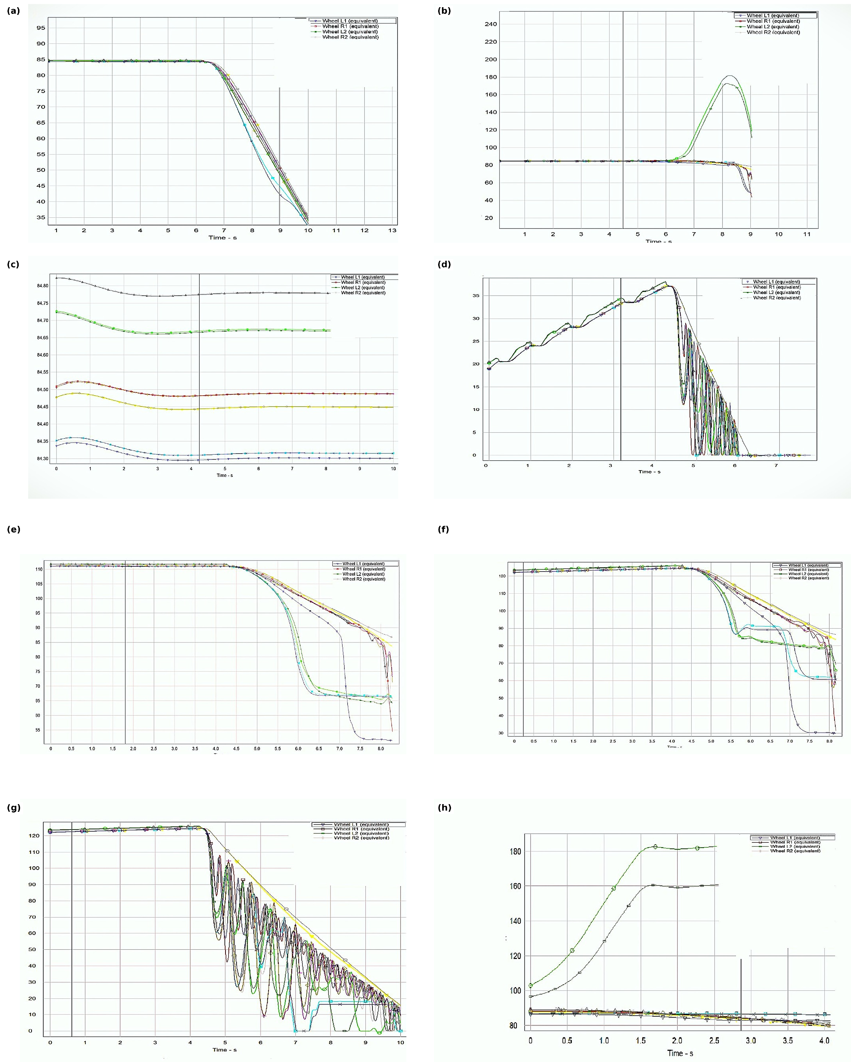
Figure 6 illustrates eight representative faulty wheel speed sensor scenarios generated in the TruckSim–Simulink co-simulation environment. Each plot demonstrates a distinct anomaly in wheel speed dynamics resulting from faulty input behavior, such as irregular brake pressure, excessive steering angles, or throttle perturbations. These abnormal driving inputs force TruckSim to produce physically consistent yet faulty sensor responses that mimic real-world ABS malfunctions. The variation in wheel speed profiles across the eight scenarios highlights diverse fault characteristics as illustrated in Table 2. Such diversity ensures that the faulty dataset captures a comprehensive range of realistic failure modes for robust TCN model training and validation.

This fault modeling approach ensures consistency between the responses of the physical vehicles and their corresponding sensor outputs. Consequently, the co-simulation environment produces a rich dataset encompassing both normal and faulty operating conditions, which are subsequently utilized for TCN model training, validation, and FPGA-based fault detection mechanism implementation.

4.3. TCN Architecture and Dual Learning Framework

The classifier used conditional log-likelihood from sequences of input signals that are below a time-varying limit. When dealing with time-series data, networks must effectively capture and retain long-term dependencies. To achieve this, dilated convolutions is used, allowing the network to reach an exponentially large receptive field using only a limited number of layers [26].

In this context, dilation refers to the inserting of fixed gaps between the elements of the convolution kernel. By spacing these elements apart, the model captures both short- and long-range temporal patterns without a proportional increase in computational cost.

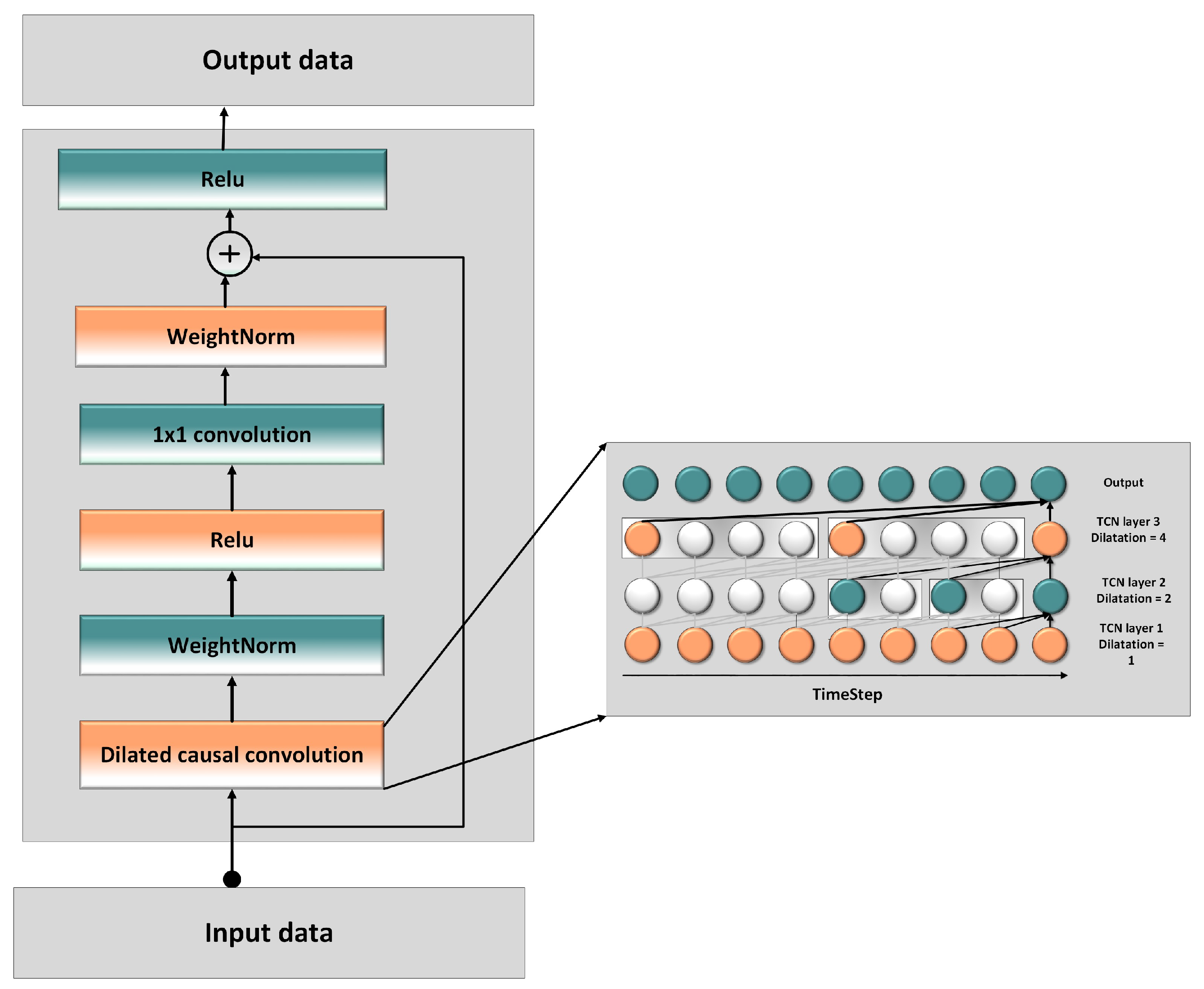
The architecture of a TCN is built upon stacked residual blocks. As illustrated in Figure 7, the input data sequentially passes through multiple Temporal Convolutional Modules (TCMs). Each TCM layer employs a dilated causal convolution, ensuring that the outputs depend only on the past and present inputs. The dilation factor increases exponentially with network depth (e.g., 1, 2, 4), which rapidly expands the receptive field and enables the network to model long-range dependencies. Within each module, the core operations typically include a dilated causal convolution, followed by Weight Normalization, a ReLU activation function, and a $1\times 1$ convolution. This configuration allows the TCN to efficiently process sequential data while maintaining temporal causality.

The receptive field R of a TCN defines the number of input time steps that influence a single output value and is expressed as:

$$R=1+\sum _{l=1}^L\left(k^{\left(l\right)}-1\right)·d^{\left(l\right)}$$

(8)

where:

• L: number of TCN layers;
• $k^{\left(l\right)}$: kernel size at layer l;
• $d^{\left(l\right)}$: dilation factor at layer l.

For the TCN configuration used in this study (Figure 7), the model was designed to capture multi-scale temporal dependencies essential for accurate wheel speed prediction. A kernel size of $k=3$ and $L=3$ layers were used, with dilation factors of 1, 2, and 4, respectively. This structure provides a receptive field sufficient to model both immediate and delayed temporal relationships. The model was trained for 140 epochs using the Adam optimizer for efficient convergence.

Unlike conventional recurrent architectures, a TCN ensures strict causality, which means that each prediction depends only on past and present inputs, preventing information leakage from future data. Furthermore, TCNs can map variable-length input sequences to equal-length output sequences, making them particularly suitable for time-series modeling [27].

A TCN predicts the next l values in a given time series. For an input sequence $x_0,x_1,\dots ,x_L$, the model produces a corresponding output sequence $y_0,y_1,\dots ,y_L$, where each $y_t$ represents the input shifted forward by l time steps. At any time step t, the model can only utilize the inputs $x_0,x_1,\dots ,x_t$ to predict $y_t$, thus maintaining temporal consistency.

In this work, the proposed dual-learning TCN framework operates under two complementary inference modes: open-loop and closed-loop. During initialization, the model functions in open-loop mode, where the first 40 input samples (referred to as the seed sequence) are directly fed from the sensor dataset. Once the initial states are established, the system transitions to closed-loop operation, in which subsequent predictions are generated autonomously based on previously predicted outputs rather than new sensor inputs.

This closed-loop configuration allows the model to emulate the temporal evolution of the wheel speed sensor behavior in real time, enabling accurate prediction and fault detection even in the absence of live input data. The choice of a 40-sample seed window was determined through analysis of both the temporal characteristics of the wheel speed signal and the receptive field of the TCN architecture. At a sampling rate of 60 Hz, this corresponds to approximately 0.67 s of sensor data, which encompasses a complete braking transient and provides sufficient temporal context for stable state initialization.

Moreover, since the TCN receptive field is 15 samples for the selected kernel and dilation parameters (as derived from the receptive field Equation (1) with $L=3$ convolutional layers and dilation factors $d=[1,2,4]$), using a 40-sample seed approximately three times larger than the receptive field ensures complete coverage of short- and mid-term temporal dependencies while maintaining low latency and efficient FPGA resource utilization.

The performance of the proposed TCN model is primarily evaluated using two error metrics, the MSE and the MAE. The MSE measures the average squared difference between the predicted outputs of the model and the actual sensor values, while the MAE quantifies the average absolute difference between them.

A lower MSE or MAE indicates a closer match between the predicted and actual sensor readings, reflecting the model’s ability to accurately capture the temporal dynamics of the system. Minimizing this metric during training ensures that the model effectively learns the underlying temporal correlations and reproduces realistic sensor behavior.

Based on this architecture, a dual-learning model was developed based on two independently trained TCNs, one modeling the behavior of the normal wheel speed sensor and the other modeling faulty behavior. The normal model was trained exclusively on datasets representing normal sensor operation, while the faulty model was trained on 5000 samples representing eight different fault conditions (

Table 4. Distribution of fault types in 5000 samples.

Fault Type	Number of Samples	Percentage (%)
1	625	12.5
2	630	12.6
3	628	12.6
4	588	11.8
5	664	13.3
6	587	11.7
7	627	12.5
8	651	13.0
Total	5000	100

). Each model learned its respective temporal dynamics from its dedicated dataset, forming the foundation of the dual-inference fault detection mechanism.

For this framework, the dataset was divided into two main classes: normal and faulty behavior. Each class was subdivided into training, validation, and test subsets. To make certain, all data were normalized by the MinMaxScaler from the scikit-learn library [28], which scales values within the range $[0,1]$:

$$Z_i={\displaystyle \frac{x_i-min\left(x\right)}{max\left(x\right)-min\left(x\right)}}$$

(9)

where $Z_i$ is the normalized value and $x_i$ represents an individual data point from the original dataset.

The training subsets were used to fit each TCN model to its respective data type, while the validation subsets supported hyperparameter tuning and overfitting prevention. Finally, the test subsets were used to assess the generalization performance of both models, allowing the framework to classify incoming wheel speed sensor data as normal or faulty based on temporal pattern matching and reconstruction errors.

The datasets used to train both models were generated in a TruckSim–Simulink co-simulation environment, where abnormal driving behaviors were intentionally induced by forcing TruckSim to operate under abnormal input conditions. These included modified control commands such as abnormal brake pressure profiles, irregular steering angles, and vehicle speed. Through the manipulation of these input signals, the simulated truck was driven to dynamic conditions that emulate sensor anomalies.

Table 5. TruckSim parameters used for ABS TCN model dataset generation.

Variable Name	Description	Unit	Role
Pbk_Con	Brake pressure command	Unitless ([−1, 0])	Input
Steer_SW	Steering wheel angle	(°)	Input
ABS_L1 to ABS_L5	ABS control state for five left wheels	Boolean	Input
ABS_R1 to ABS_R5	ABS control state for five right wheels	Boolean	Input
GearStat	Gear status	Integer	Input
Throttle	Throttle pedal position	Unitless ([0, 1])	Input
Vx	Longitudinal speed	km/h	Output
AVz	Yaw rate	°/s	Output
AVz_2	Yaw rate (trailer)	°/s	Output
Ay	Lateral acceleration	m/s2	Output
Ay_2	Lateral acceleration (trailer)	m/s2	Output
Fs	Mean wheel load (front/rear, left/right)	N	Output
Roll	Roll angle	(°)	Output
Vx_L1 to Vx_L5	Five left wheel speeds	km/h	Output
Vx_R1 to Vx_R5	Five right wheel speeds	km/h	Output

summarizes the TruckSim parameters used to generate normal and faulty datasets. These parameters were selected to capture the comprehensive dynamics of the vehicle under varying conditions. The input variables (e.g., brake pressure command, steering wheel angle, throttle position, and ABS control states) act as control signals that influence vehicle dynamics, while the output variables (e.g., longitudinal speed, yaw rate, lateral acceleration, and individual wheel speeds) represent the measurable system responses that the TCN models are trained to predict.

4.4. Fault Detection Stage

In this stage, each incoming wheel speed signal is simultaneously fed to both TCN models. The normal TCN attempts to reconstruct the expected sensor signal under nominal operating conditions, whereas the faulty TCN predicts the corresponding behavior under fault-induced conditions.

For each model, the reconstruction errors are computed using both the MSE and the MAE:

$${\mathrm{MSE}}_{\mathrm{normal}}={\displaystyle \frac{1}{n}}\sum _{i=1}^n{(y_i-{\widehat{y}}_{i,\mathrm{normal}})}^2,{\mathrm{MSE}}_{\mathrm{faulty}}={\displaystyle \frac{1}{n}}\sum _{i=1}^n{(y_i-{\widehat{y}}_{i,\mathrm{faulty}})}^2$$

(10)

$${\mathrm{MAE}}_{\mathrm{normal}}={\displaystyle \frac{1}{n}}\sum _{i=1}^n|y_i-{\widehat{y}}_{i,\mathrm{normal}}|,{\mathrm{MAE}}_{\mathrm{faulty}}={\displaystyle \frac{1}{n}}\sum _{i=1}^n|y_i-{\widehat{y}}_{i,\mathrm{faulty}}|$$

(11)

where $y_i$ denotes the measured wheel speed at time step i, and ${\widehat{y}}_{i,\mathrm{normal}}$ and ${\widehat{y}}_{i,\mathrm{faulty}}$ are the predictions from the normal and faulty TCN models, respectively.

Both MSE and MAE have probabilistic interpretations. Minimizing MSE corresponds to maximizing the likelihood under Gaussian noise:

$${\mathcal{L}}_{\mathrm{MSE}}\propto -\sum _{i=1}^{n}log\left(e^{-{\displaystyle \frac{{(y_i-{\widehat{y}}_i)}^2}{2{\sigma }^2}}}\right),$$

(12)

while minimizing MAE corresponds to maximizing the likelihood under Laplacian noise:

$${\mathcal{L}}_{\mathrm{MAE}}\propto -\sum _{i=1}^{n}log\left(e^{-{\displaystyle \frac{|y_i-{\widehat{y}}_i|}{b}}}\right).$$

(13)

Reporting MSE and MAE separately provides complementary information: MSE emphasizes large deviations critical for detecting abrupt faults, whereas MAE captures consistent small errors and noise-driven variations.

The final classification decision is made by comparing the two models independently on both metrics:

$$\mathrm{Decision}=\left\{\begin{array}{cc}\mathrm{Normal}\mathrm{behavior},\hfill & \mathrm{if}{\mathrm{MSE}}_{\mathrm{normal}}<{\mathrm{MSE}}_{\mathrm{faulty}}\mathrm{and}{\mathrm{MAE}}_{\mathrm{normal}}<{\mathrm{MAE}}_{\mathrm{faulty}},\hfill \\ \mathrm{Faulty}\mathrm{behavior},\hfill & \mathrm{otherwise}.\hfill \end{array}\right.$$

(14)

This dual-metric strategy leverages the complementary strengths of both error measures and model types to accurately distinguish normal and faulty temporal patterns. When implemented on FPGA, it enables real-time, low-latency fault detection and correction, forming the foundation for hardware-accelerated ABS ECU validation and diagnostic testing.

4.5. FPGA-Based Prediction Module

FPGAs offer a reconfigurable and parallel processing environment well-suited for real-time control and HIL simulations. Their ability to execute concurrent operations enables the implementation of complex neural network architectures such as TCNs for rapid signal analysis, fault recognition, and closed-loop system validation.

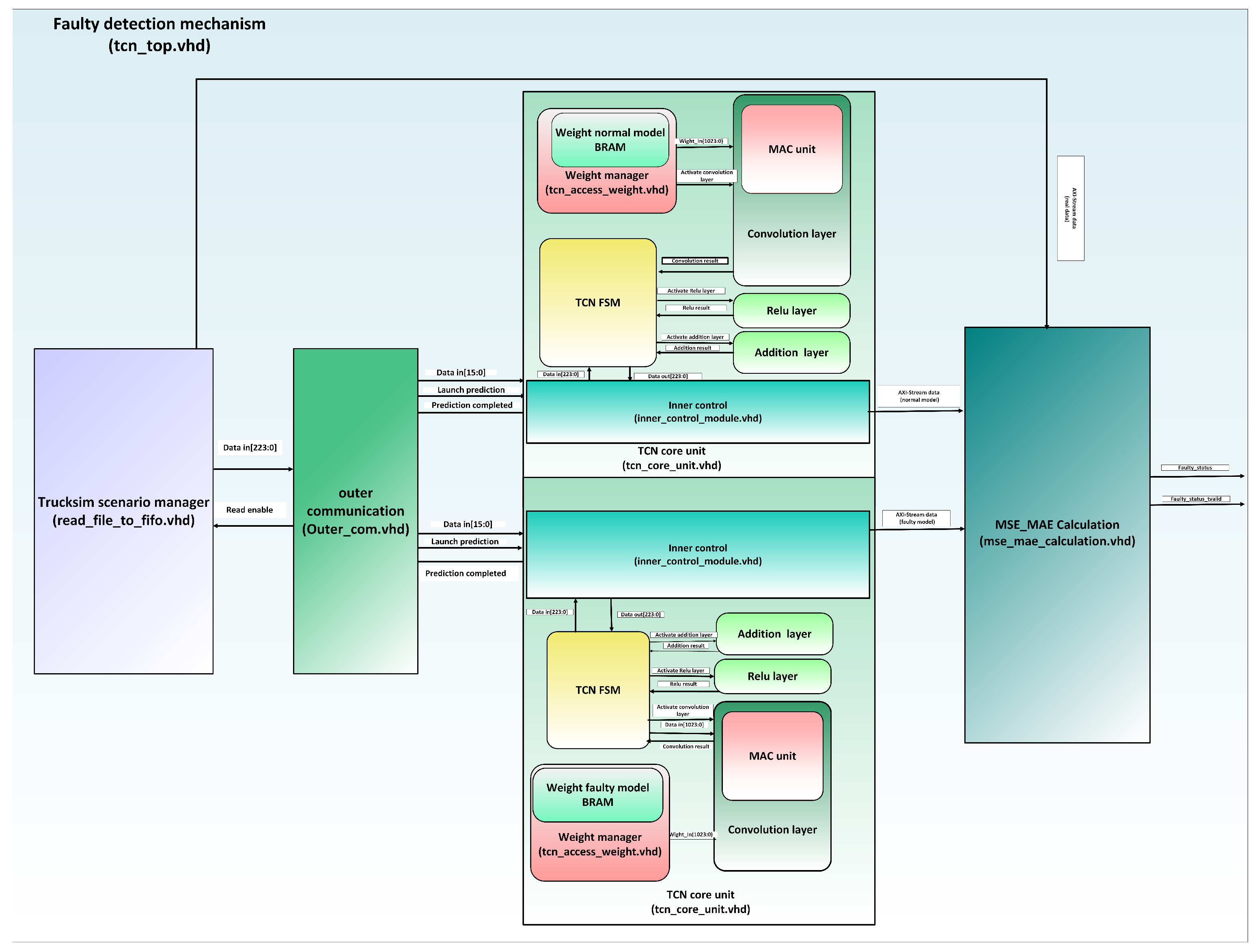
In the proposed system, the FPGA acts as an intelligent module for real-time fault early sensor-level detection in the HIL simulation platform for ABS systems. It performs real-time data monitoring, prediction, and fault classification within the HIL loop. The FPGA implementation, shown in Figure 8, is composed of four principal subsystems: the TCN prediction model module and the Fault detection module.

TCN Prediction Model

A key step in the hardware implementation involves mapping the trained parameters of both the normal and faulty TCN models onto the FPGA’s on-chip memory resources. The pre-trained weights and biases obtained from Python-based GPU training are quantized into a fixed-point Q1.15 format and exported as Coefficient (.coe)  files. These files are used to initialize the FPGA’s embedded Block RAMs (BRAMs) during bitstream generation, ensuring that model parameters are directly accessible from dedicated on-chip memory. This approach eliminates the latency associated with external memory access and enables parallel weight retrieval during convolution operations.

The TCN dual-weight model manager organizes and controls two independent BRAM blocks that store the pre-trained parameters of the normal and faulty TCN models, respectively. A multiplexer (MUX) dynamically selects the active weight bank according to the operational mode or testing scenario defined by the TruckSim scenario manager. This architecture allows seamless, real-time switching between normal and faulty model evaluations within the FPGA fabric, without requiring hardware reconfiguration or interrupting the HIL simulation.

The TruckSim scenario manager dynamically selects either normal or faulty vehicle dynamics scenarios from TruckSim CSV file based on the input and output parameters summarized in Table 5. These scenarios represent diverse braking conditions and sensor degradation profiles, ensuring a comprehensive range of test environments.

In the closed-loop configuration, the TruckSim scenario manager streams real-time wheel speed data to the FPGA-based TCN prediction module through a dedicated input channel. During the first 40 sampling intervals, the model operates in open-loop mode to initialize its internal temporal states and synchronize with the vehicle’s dynamics.

After this warm-up phase, the system transitions to closed-loop prediction, where the TCN’s previously predicted outputs are used as inputs for subsequent time steps to predict the next-step outputs. This feedback strategy enhances prediction stability and accuracy under transient conditions and sensor faults, enabling reliable real-time estimation of wheel speed behavior under both normal and faulty scenarios.

The TCN finite-state machine (FSM) orchestrates the overall data flow and synchronization among the convolution, activation, and accumulation stages for both models, ensuring deterministic timing and proper sequencing of input loading, weight access, and output generation for real-time inference on the FPGA. The controller is implemented as a synchronous Moore FSM with 17 states, driven by eight logical inputs (network_input_tvalid, fc_conv_result_tvalid, relu_result_tvalid, addition_result_tvalid, load_causal_activations, and resetn) and generating twelve registered outputs (handshake, layer-activation, block-selection, and output-valid/data signals). This Moore-style implementation was chosen because all control signals depend only on the current state, which avoids combinational glitches, simplifies timing closure, and guarantees deterministic cycle-by-cycle behavior.

The TCN layer comprises three computational blocks: a convolution layer for temporal feature extraction, a ReLU layer for non-linear activation, and an addition layer for residual accumulation. The convolution layer is implemented using a dedicated multiply–accumulate (MAC) unit, which performs temporal convolutions across input sequences to capture dynamic dependencies in the wheel speed signals. Under FSM supervision, the MAC unit executes pipelined and parallel computations with minimal latency.

As one of the most resource-intensive modules in neural network accelerators, the MAC unit performs numerous multiply-and-add operations across neurons and layers, consuming significant FPGA resources such as DSP slices, LUTs, and flip-flops. Efficient design and optimization of the MAC are therefore critical to balancing computational precision, throughput, and resource utilization.

To address these challenges, an optimized fixed-point MAC (OFM) architecture is adopted in this work to enhance performance while minimizing FPGA resource consumption [29]. The OFM unit, illustrated in Figure 8, consists of two main pipeline stages: a multiplication stage and an accumulation stage. Both stages operate on operands represented in the Q1.15 fixed-point format, where one bit is allocated for the integer part and fifteen bits for the fractional part. This representation provides a good balance between numerical precision and hardware efficiency, making it well-suited for real-time ABS sensor signal prediction and HIL-based testing applications.

The outputs from the TCN prediction models are routed to the MSE calculation module, which differentiates between the results generated by the normal and faulty models and computes the MSE for each output parameter according to Table 5 for both normal and faulty models.

Utilizing Equation (14) together with the calculated MSE and MAE metrics, the early sensor-level fault detection module identifies abnormal sensor behavior and triggers alerts to prevent corrupted data from being transmitted to the ECU.

The combination of FSM-based control, dual-weight management, optimized MAC computation, and fault detection logic ensures deterministic timing, low latency, and scalability for multi-sensor configurations. These characteristics make the proposed design particularly suitable for real-time wheel speed sensor fault detection in safety-critical ABS applications.

5. Experimental Setup

This section describes the HIL test platform developed to evaluate the Bendix EC-60 ABS ECU under both normal and faulty wheel-speed sensor conditions. As illustrated in Figure 9, the platform integrates the FPGA-based fault-detection mechanism shown in Figure 2 as a core component within a real-time simulation and data-acquisition framework. The objective of the HIL setup is twofold: (i) to verify that the ECU correctly detects and reacts to abnormal sensor behavior injected by the TCN-based virtual sensor and (ii) to confirm that, under non-faulty conditions, the Bendix EC-60 operates correctly without spurious fault activation.

The HIL platform is composed of four major hardware subsystems that form a closed-loop testing environment, corresponding to the blocks shown in Figure 9:

• FPGA fault-detection module: hosts the fixed-point implementation of the TCN model for real-time sensor data processing and fault detection. Wheel speed time series generated by the Trucksim simulator are buffered in the BRAM on programmable logic (PL) of ZCU102 board. The PL then processes these samples with the TCN, and the resulting predicted wheel speed values and fault flags are passed back through AXI-Stream FIFOs between the PL and PS before being transferred to the simulator over USB 3.0 for further use in the HIL loop.
• Signal-generation module: converts the FPGA’s digital predicted wheel speed sensors into analog wheel speed sensor signals for the ECU.
• Signal-acquisition module: uses A/D convertors on the same backplane, wired to the ECU outputs such as Pressure Modulating Valves (PMVs), Traction Control Valves (TCVs), and status lines. These channels continuously record the ECU’s reaction to the injected wheel speed profiles and faults and stream the data back to the host PC for logging and offline analysis.
• Communication interface module: manages J1939/CAN bus data exchange between the ECU and the host system.

All modules are interconnected via the simulator’s custom-designed backplane, which integrates analog and digital I/O, the CAN interface, and the required power rails. The backplane provides a single, high-bandwidth USB 3.0 connection to the FPGA prediction module and ensures deterministic timing between signal generation, acquisition, and TCN inference, thereby guaranteeing synchronous operation of the HIL loop.

5.1. FPGA Interface and Integration

The core of the prediction module is a Xilinx ZCU102 evaluation board integrating a Zynq UltraScale+ MPSoC, chosen for its tightly coupled PS and PL. The architecture is shown in Figure 8. The PL executes the low-latency, parallel computations of the TCN model (convolutions and residual blocks), while the PS, equipped with ARM cores, manages high-level control, buffer management, and communication with the HIL simulator.

A key aspect of the design is the robust communication interface bridging the HIL simulator and the FPGA. The Vitis project employs a Communications Device Class (CDC) USB 3.0 interface, enabling the FPGA to appear as a virtual COM port on the host PC. This high-bandwidth link is used exclusively for real-time sensor and actuator data transfer. On the FPGA side, AXI-Stream FIFO interfaces bridge the PS and PL, decoupling the TCN computation from USB transfer latency and enabling continuous streaming of wheel-speed samples through the TCN pipeline.

During operation, wheel-speed sequences generated by the TruckSim-based simulator are sent to the FPGA via USB 3.0. The PL processes these sequences with the TCN and returns predicted wheel-speed values and corresponding fault indicators to the PS, which forwards them back to the simulator. The signal-generation module then converts these predictions into analog wheel-speed signals, which are applied to the EC-60 ECU. The ECU executes its ABS control logic based on these signals, modulating PMVs and TCVs accordingly. The acquisition module records the ECU responses and forwards them to the host system for further analysis, closing the validation loop over a wide range of nominal and faulty scenarios.

5.2. ECU Signal Configuration

The interface between the HIL platform and the Bendix EC-60 ECU is defined by the input and output signals listed in

Table 6. Input and output signal configuration of the Bendix EC-60 ABS ECU.

Category	Signal	Description
Inputs	Wheel Speed Sensors (Steering-LH, Steering-RH, Drive1-LH, Drive1-RH, Drive2-LH, Drive2-RH)	Measure wheel-end speed on each side of the front and rear axles. Dual tires on a single axle end are represented by one sensor.
	Brake Pressure Sensor	Provides real-time brake pressure feedback for closed-loop control accuracy.
Outputs	Pressure Modulating Valves (PMV-Steering-LH, PMV-Steering-RH, PMV-Drive1-LH, PMV-Drive1-RH, PMV-Drive2-LH, PMV-Drive2-RH)	Regulate braking pressure at each wheel-end to prevent wheel lock-up during braking.
	Traction Control Valves (TCV-Drive1-LH, TCV-Drive1-RH, TCV-Drive2-LH, TCV-Drive2-RH)	Engage traction control by applying selective braking to restore grip during wheel slip events.

. While a commercial truck may include up to ten wheel speed sensors, the EC-60 ECU simplifies this by using six—one per side on the steering and drive axles—ensuring full axle-end coverage without redundancy. The outputs consist of corresponding PMVs and TCVs that regulate braking pressure and traction control at each wheel end.

6. Results and Discussion

To evaluate the proposed system, we verified that the dual-learning model effectively distinguishes between normal and faulty wheel speed sensor behaviors. The underlying principle is that each TCN model should achieve the lowest prediction error on the type of data it was trained on. Consequently, for normal sensor data, the normal-behavior TCN is expected to produce a lower prediction error than the faulty-behavior TCN, and vice versa. This comparative evaluation enhances both the robustness and precision of the fault detection framework.

Formally, let ${\mathrm{MSE}}_{\mathrm{normal}}$ and ${\mathrm{MSE}}_{\mathrm{faulty}}$ denote the Mean Squared Errors obtained from the normal and faulty TCN models, respectively. Similarly, let ${\mathrm{MAE}}_{\mathrm{normal}}$ and ${\mathrm{MAE}}_{\mathrm{faulty}}$ represent the corresponding Mean Absolute Errors. The individual decision metrics are first evaluated for each model to quantify the reconstruction quality of the input sequence.

Since the MSE metric is highly sensitive to large deviations, it is particularly effective for identifying abrupt or severe anomalies in wheel speed sensor signals. In contrast, the MAE metric provides a more uniform weighting of all errors, offering robustness against isolated outliers or transient disturbances. By jointly analyzing both metrics, the framework leverages the complementary characteristics of MSE and MAE to improve overall fault discrimination accuracy.

The final classification decision is made by comparing the error magnitudes from both TCN models, as given in Equation (14).

In practice, the joint MSE–MAE evaluation enhances decision reliability by reducing sensitivity to noise and preventing false detections caused by short-term fluctuations. During real-time FPGA deployment, this rule enables the early sensor-level fault detection module to dynamically select the most representative model (normal or faulty) based on the reconstruction consistency of incoming wheel speed signals. Consequently, the system achieves robust and adaptive fault classification across diverse driving and fault conditions.

6.1. Evaluation Based on Classification Metrics

In addition to the error-based decision rules, the classification performance of the proposed fault detection framework was evaluated using standard metrics derived from the confusion matrix, as summarized in

Table 7. Performance metrics based on confusion matrix [30].

Metric	Definition	Formula
Accuracy	Proportion of correct predictions	${\displaystyle \frac{\mathrm{TP}+\mathrm{TN}}{\mathrm{TP}+\mathrm{TN}+\mathrm{FP}+\mathrm{FN}}}$
Precision (PPV)	Proportion of positive predictions that are correct	${\displaystyle \frac{\mathrm{TP}}{\mathrm{TP}+\mathrm{FP}}}$
Recall (Sensitivity)	Proportion of actual positives correctly identified	${\displaystyle \frac{\mathrm{TP}}{\mathrm{TP}+\mathrm{FN}}}$
Specificity	Proportion of actual negatives correctly identified	${\displaystyle \frac{\mathrm{TN}}{\mathrm{TN}+\mathrm{FP}}}$
F1-Score	Harmonic mean of precision and recall	${\displaystyle \frac{2\mathrm{TP}}{2\mathrm{TP}+\mathrm{FP}+\mathrm{FN}}}$

. A classification outcome is defined as follows:

• True Positive (TP): Faulty input correctly identified as faulty.
• True Negative (TN): Normal input correctly identified as normal.
• False Positive (FP): Normal input incorrectly classified as faulty.
• False Negative (FN): Faulty input that is not detected.

The performance of the fault detection model was evaluated by increasing size of datasets, each model containing an equal number of normal and faulty samples to ensure class balance. A 70%/20%/10% split was applied for training, validation, and testing, respectively, resulting in approximately 500 normal and 500 faulty samples in the test set for the 5000-sample configuration.

The results, summarized in

Table 8. Performance metrics for fault detection models with different dataset sizes.

Dataset Size	TP	FP	TN	FN	Accuracy	Precision	Recall	F1-Score
2000	156	57	143	44	0.748	0.733	0.780	0.756
3000	253	62	238	47	0.805	0.803	0.843	0.823
4000	356	54	346	44	0.880	0.868	0.890	0.879
5000	467	55	445	33	0.912	0.894	0.934	0.914
7000	637	77	623	63	0.910	0.892	0.910	0.901

, show that increasing the dataset size improves the model’s overall performance across all metrics. Performance peaks at the 5000-sample dataset, achieving an accuracy of 0.912 and an F1-score of 0.914. Expanding the dataset further to 7000 samples results in a marginal performance decrease (F1-score of 0.901), indicating that the model converges and additional data provide diminishing returns.

These classification metrics complement the error-based measures (MSE and MAE). While error metrics quantify the magnitude of prediction deviations, precision, recall, and F1-score assess the system’s classification effectiveness. Together, they provide a comprehensive evaluation of the dual-learning fault detection framework under various dataset scales and driving conditions.

6.2. Comparative Analysis: Dual-TCN vs. Single-TCN Framework

To provide an initial comparison, a single-TCN model was implemented using only the normal behavior scenarios. In this configuration, the model predicts the expected wheel speed sequence and computes the MSE between the predicted and measured signals. A fault is detected when the prediction error exceeds a predefined MSE threshold.

To determine the fault detection threshold for the single-TCN model, the MSE distribution of the validation dataset was analyzed using samples from the 5000-sample configuration, which included both normal and faulty data sequences. The validation subset consisted exclusively of normal samples (approximately 500) to ensure that the threshold reflected the expected variability of prediction errors under healthy sensor conditions. The mean (${\mu }_{\mathrm{val}}$) and standard deviation (${\sigma }_{\mathrm{val}}$) of the MSE values were computed from these normal samples, and the threshold was defined according to the well-established k-sigma method [31,32]:

$${\mathrm{Threshold}}_{\mathrm{MSE}}={\mu }_{\mathrm{val}}+k·{\sigma }_{\mathrm{val}},$$

(15)

where k is a positive sensitivity factor chosen empirically, ${\mu }_{\mathrm{val}}$ represents the expected prediction error for normal sensor behavior, and ${\sigma }_{\mathrm{val}}$ quantifies its variation across different driving conditions.

The k-sigma method is a widely used and straightforward statistical approach for threshold selection. In this study, empirical analysis showed that $k=2.5$ provided an effective trade-off between sensitivity and stability.

Using the test scenarios from the normal model (${\mu }_{\mathrm{val}}=0.00597$) and the estimated standard deviation (${\sigma }_{\mathrm{val}}\approx 0.0035$), the resulting threshold was computed as:

$${\mathrm{Threshold}}_{\mathrm{MSE}}=0.00597+2.5\times 0.0035=0.0147.$$

(16)

Consequently, any wheel speed signal producing an MSE above 0.0147 was statistically classified as faulty. If the instantaneous MSE exceeded this limit over a consecutive window of samples, the system flagged the sensor as faulty; otherwise, it was considered normal.

For comparative evaluation, both the single-TCN and the proposed dual-TCN frameworks were tested under identical conditions. Each model was evaluated using 1000 test samples (500 normal and 500 faulty) derived from the 5000-sample dataset to ensure a fair and balanced comparison. Detection performance was quantified using metrics such as accuracy, precision, recall, and F1-score.

The results in

Table 9. Performance comparison between single-TCN and dual-TCN approaches.

Metric	Single-TCN	Dual-TCN (Proposed)
Detection Accuracy (%)	91.4	97.8
Precision (%)	89.2	96.5
Recall (%)	88.7	98.2
F1-Score (%)	88.9	97.3

clearly demonstrate that the dual-TCN framework outperforms the single-TCN approach across all evaluation metrics. While the single-TCN relies on a fixed MSE threshold, the dual-TCN leverages a comparative learning strategy between the normal and faulty networks, enabling adaptive and threshold-free classification.

6.3. Case Studies

To further demonstrate the comparative mechanism of the dual model, we present two case studies from TruckSim simulation scenarios: one under normal conditions and another with a simulated fault.

6.3.1. Case Study 1 (Normal Scenario)

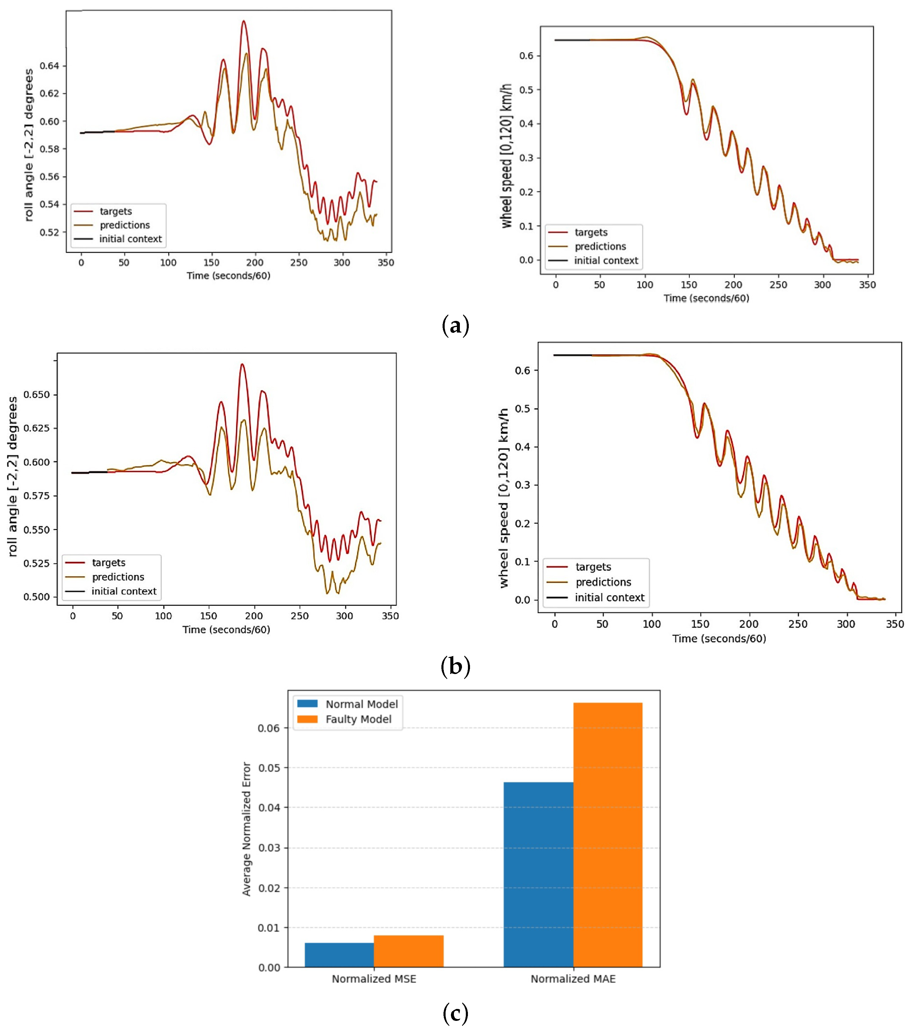
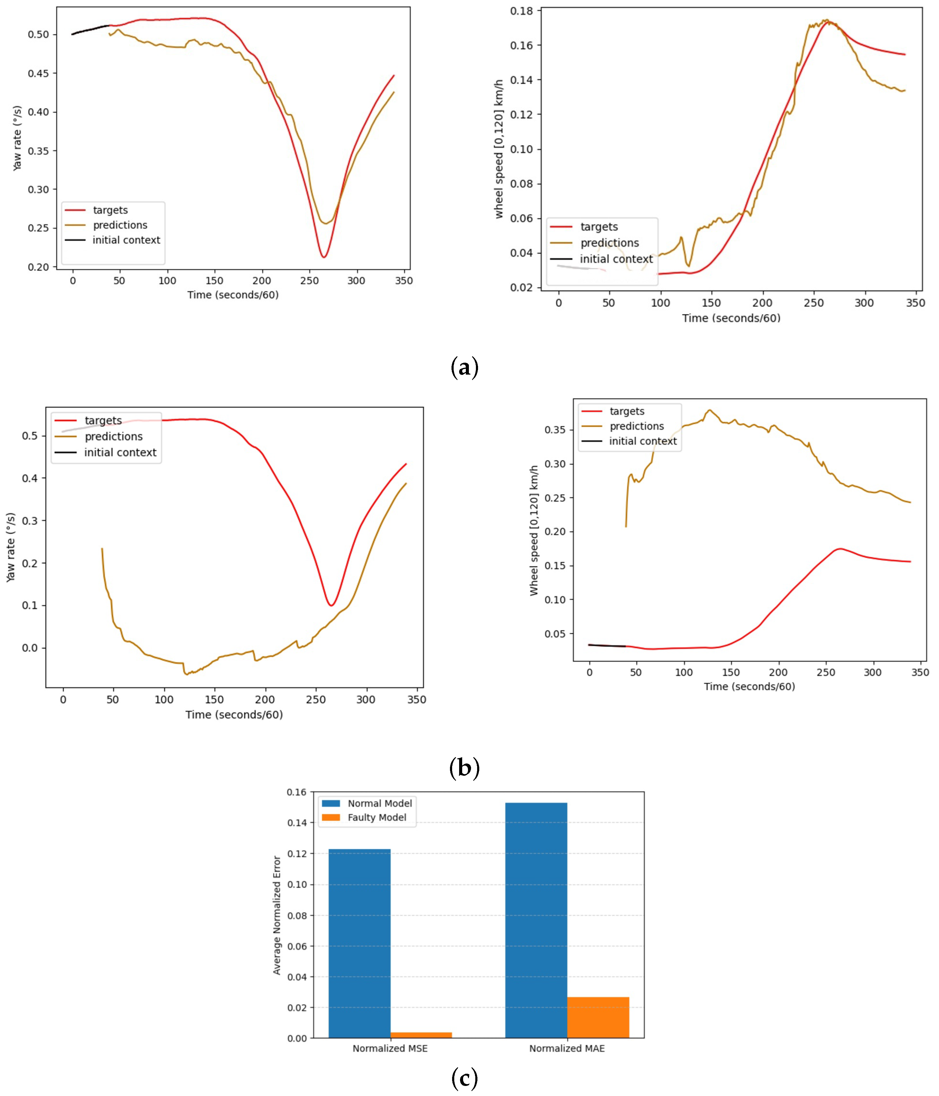
Figure 10 illustrates the model performance under normal driving conditions. In this scenario, normal sensor data were applied to both the normal-behavior model and the faulty-behavior model. As shown in Figure 10b, the predictions generated by the normal model closely follow the target signals across all two variables (roll angle, and wheel speed), indicating a tight alignment and low prediction error. In contrast, the faulty-behavior model in Figure 10a shows noticeable deviations between the predicted and actual signals, particularly during later time intervals, reflecting larger and more variable errors.

The comparison in Figure 10c quantitatively supports this observation. Both the normalized MSE and MAE are significantly lower for the normal model compared to the faulty model. This confirms that the framework correctly recognizes normal operating conditions by assigning smaller and more consistent errors to the appropriate model, while the faulty model exhibits a broader spread of errors due to its inability to capture the normal behavior pattern.

6.3.2. Case Study 2 (Faulty Scenario)

Figure 11 presents the model performance when faulty sensor data were applied to both TCN models. As illustrated in Figure 11a, the faulty behavior model shows strong predictive accuracy, with predicted signals closely matching the actual target values across all measured parameters. In contrast, the normal behavior model shows a clear mismatch between predicted and target signals, especially during dynamic transitions, indicating that it fails to represent the fault pattern accurately.

The quantitative results in Figure 11c reinforce this finding. The faulty behavior model achieves substantially lower normalized MSE and MAE values, while the normal model yields higher and more dispersed errors, reflecting its inability to adapt to abnormal behavior. This reversal of results, compared with the normal scenario, validates the framework’s capability to effectively discriminate between healthy and faulty conditions by assigning lower errors to the corresponding model.

To evaluate the hardware feasibility of the proposed dual-TCN fault detection framework, the design was synthesized and implemented on an FPGA platform. Resource utilization was analyzed to assess computational and memory efficiency during real-time execution.

The synthesis results summarized in

Table 10. FPGA resource utilization summary for the implemented TCN-based fault detection architecture.

Resource	Estimation	Available	Utilization (%)
LUT	34,815	274,080	12.70
LUTRAM	6	144,000	0.01
FF	109,935	548,160	20.06
BRAM	174	912	19.08
DSP	128	2520	5.08
IO	22	328	6.71
BUFG	1	404	0.25

show that the proposed dual-TCN architecture occupies 12.7% of LUTs, 20.1% of FFs, 19.1% of BRAMs, and 5.1% of DSP slices, with negligible LUTRAM (0.01%) and BUFG (0.25%) usage. This relatively low utilization is important for several reasons, even though the full FPGA device is already present on the PCB.

First, it demonstrates that the proposed architecture is computationally efficient and does not require a high-end device: the same design could be migrated to a smaller and less expensive FPGA or integrated alongside additional logic on the same SoC, which is relevant for industrial deployment and cost optimization. Second, the available resource headroom provides a clear path for scalability. In future work, we plan to extend the platform beyond ABS to include additional ECU fault-detection modules (e.g., steering, transmission, or powertrain). The current FPGA leaves sufficient LUT, BRAM, and DSP capacity to instantiate further TCN-based monitors or higher-capacity models without redesigning the hardware platform.

Third, although the static power is dominated by the device itself, keeping the design compact reduces dynamic power by limiting the number of actively switching LUTs, FFs, BRAMs, and DSPs, which is beneficial when the FPGA also hosts other time-critical tasks. Overall, Table 10 does not simply show that resources are “unused”, but rather that the proposed dual-TCN implementation achieves real-time performance with a modest hardware footprint, leaving ample margin for future extensions, additional ECU monitoring blocks, and integration into cost- and power-constrained automotive platforms.

From a timing perspective, the dual-TCN block operates as a supervisory monitor running in parallel with the ABS ECU. The ECU preserves its original control period of 16.7 microsecond (60 Hz), while the TCN accelerator on the FPGA processes the same wheel-speed measurements and produces a fault/normal decision without altering the ECU’s actuation schedule. Owing to the fully pipelined hardware implementation, the end-to-end latency from input-window arrival to fault decision is on the order of only a few tens of microseconds (i.e., well below 1% of ABS control cycle). As a result, the additional monitoring introduces only minimal latency and has no practical impact on the timing or stability of the ABS control loop, while still enabling real-time sensor health assessment.

6.4. Bendix EC60 Results Under Normal and Faulty Wheel Speed Sensor Conditions

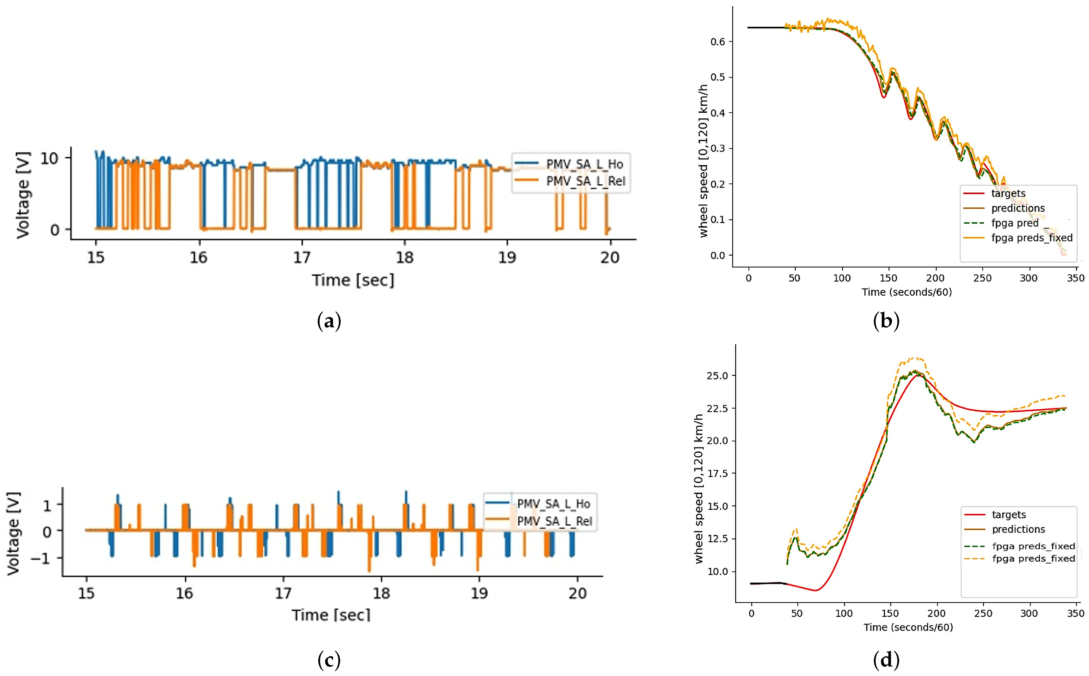
Figure 12 illustrates the feedback obtained from the Bendix EC-60 ABS ECU under normal and faulty wheel speed sensor conditions. In the normal scenario, the wheel speed signal demonstrates smooth and consistent behavior, closely following the expected rotational dynamics of the wheel. This indicates that the sensor is functioning correctly, providing reliable input to the ABS ECU for effective braking control. Under these conditions, the hold signal engages the brake pressure when wheel slip exceeds the ABS threshold. The release signal reduces brake pressure when the wheel regains traction. Because the wheel speed sensor provides accurate feedback, these signals are properly timed, ensuring smooth braking and preventing wheel lock-up.

Conversely, the faulty scenario exhibits noticeable deviations from the expected wheel speed profile. The signal may show abrupt fluctuations, drops, or spikes, which can lead to incorrect ABS responses if left uncorrected. In this case, the hold signal may engage too early or too late, causing unnecessary or insufficient brake pressure. The release signal may fail to reduce brake pressure on time, increasing the risk of wheel lock-up. Comparing these two figures highlights the impact of sensor faults on system behavior, emphasizing the importance of early fault detection.

6.5. Summary of Experimental Findings

The experimental results collectively demonstrate the effectiveness and practicality of the proposed dual-TCN framework for early sensor-level fault detection in ABS systems. First, the analysis of different dataset sizes (Table 8) shows that increasing the number of simulated sequences from 2000 to 5000 samples steadily improves all classification metrics. The best trade-off is obtained with the 5000-sample configuration, which achieves an accuracy of 0.912, a precision of 0.894, a recall of 0.934, and an F1-score of 0.914 on a balanced test set. Beyond this point (7000 samples), the performance gains become marginal, indicating that the proposed training pipeline reaches a stable generalization regime.

Second, the comparative study between the single-TCN and dual-TCN configurations (Table 9) highlights the benefit of explicitly learning both normal and faulty behaviors. Whereas the single-TCN model, relying on a fixed MSE threshold, achieves a detection accuracy of 91.4% and an F1-score of 88.9%, the proposed dual-TCN scheme reaches 97.8% accuracy, 96.5% precision, 98.2% recall, and a 97.3% F1-score under the same test conditions. This corresponds to an improvement of 6.4 percentage points in accuracy and 8.4 percentage points in F1-score, confirming that the dual-learning strategy significantly enhances fault discrimination capability.

Third, the case studies based on TruckSim scenarios (Figure 10 and Figure 11) and the Bendix EC-60 HIL experiments (Figure 12) demonstrate that these quantitative gains translate into meaningful behavior at system level. Under normal conditions, the normal-TCN model yields consistently lower MSE and MAE values than the faulty model, while under faulty conditions the situation is reversed. In the HIL tests with the EC-60 ECU, the framework correctly differentiates healthy and faulty wheel speed sensor behaviors and reflects these differences in the ECU’s PMV/TCV actuation patterns.

Finally, the FPGA implementation results (Table 10) confirm that the dual-TCN architecture can be deployed in real time with modest hardware overhead. The design uses only 12.7% of LUTs, 20.1% of flip-flops, 19.1% of BRAMs, and 5.1% of DSPs on a Xilinx ZCU102 device, while supporting streaming operation at 60 Hz within the HIL loop. This demonstrates that the proposed method is not only accurate in terms of machine learning metrics, but also feasible for embedded implementation in safety-critical automotive platforms.

Overall, the experimental findings show that the proposed dual-TCN framework delivers high detection performance, robustness across diverse fault scenarios, and efficient FPGA-based real-time execution, thereby providing a significant and practical contribution to ABS sensor fault diagnosis and ECU validation.

Beyond these results, it is important to note that, while the proposed dual-TCN framework demonstrates robustness to short-term environmental variations (e.g., loading, road surface), long-term physical changes such as tire wear or suspension degradation could, in principle, induce concept drift over multi-year operational lifetimes. This challenge is common to all data-driven automotive systems and can be addressed through periodic model retraining using updated simulation parameters, followed by FPGA bitstream updates during scheduled maintenance. Because trainings are architecturally decoupled, such updates preserve the real-time properties of the monitoring system.

7. Conclusions

This study presented a dual learning approach for intelligent early sensor-level fault detection of ABS systems. By integrating a dual-TCN model within an FPGA-based HIL simulation platform, the proposed method accurately distinguishes between normal and faulty sensor behaviors under diverse driving scenarios. Using realistic datasets generated from a TruckSim–MATLAB/Simulink co-simulation, including eight representative fault scenarios and up to 5000 labeled sequences, the framework overcomes the common limitation of scarce and non-representative faulty data.

Experimental results show that, on a balanced test set of 1000 sequences, the proposed dual-TCN framework achieves a detection accuracy of 97.8%, a precision of 96.5%, a recall of 98.2%, and an F1-score of 97.3%. In comparison, a single-TCN baseline reaches 91.4% accuracy and an 88.9% F1-score, confirming that the dual-learning strategy provides a significant improvement in fault classification performance. The complete dual-TCN architecture is implemented on a Xilinx ZCU102 FPGA, requiring only 12.7% of LUTs, 20.1% of flip-flops, 19.1% of BRAMs, and 5.1% of DSPs, while supporting real-time inference in the HIL loop with low latency.

Moreover, the FPGA-resident dual-TCN monitor introduces only negligible additional latency relative to the ABS control period, ensuring that real-time braking performance is not affected.

While the framework targets HIL-based ECU validation—where wheel-speed signals are generated virtually—its design principles address practical deployment considerations. In a physical vehicle, the dual-TCN monitor operates on the existing sensor set, learning subtle temporal anomalies without the cost, complexity, and wiring overhead of additional hardware redundancy. This makes the solution a scalable and cost-effective alternative to pure sensor duplication, with the added benefit of being reusable across multiple ECUs and vehicle subsystems.

Although this work focuses on ABS wheel-speed sensors, the same dual-TCN and FPGA-based HIL pipeline can be reused for other safety-critical ECUs by adjusting the input signals and retraining the models, making the proposed framework a generic and extensible solution for real-time fault detection in embedded automotive systems.

In summary, this work demonstrates that combining data-driven learning with hardware acceleration provides a practical, scalable solution for intelligent automotive fault detection, essential for next-generation software-defined vehicles.