A Novel Reactive Power Decoupling Strategy for VSG Inverter Systems Using Adaptive Dynamic Virtual Impedance

Abstract

Virtual synchronous machine (VSG) technology provides a robust framework for integrating electric vehicle energy storage into modern microgrids. Nonetheless, conventional VSG control often suffers from intense interaction between active and reactive power flows, which can trigger persistent steady-state errors, power fluctuations, and potential system collapse. This research addresses these challenges by developing a 5th-order electromagnetic dynamic model tailored for a two-stage cascaded bridge inverter. By synthesizing a 3rd-order power regulation loop with a 2nd-order output stage, the proposed model captures stability boundaries across an extensive parameter spectrum. Unlike traditional 3rd-order “quasi-steady-state” approaches—which overlook essential dynamics under weak-damping or low-inertia conditions—this study utilizes the 5th-order model to derive an adaptive dynamic virtual impedance decoupling technique. This strategy facilitates real-time compensation of the cross-coupling between active and reactive channels, significantly boosting the inverter’s damping ratio. Quantitative analysis confirms that this approach curtails overshoot by 85.6% and accelerates the stabilization process by 42%, markedly enhancing the overall dynamic performance of the grid-connected system.

1. Introduction

The global energy landscape is undergoing a fundamental shift, prioritizing carbon-neutral alternatives over conventional thermal power generation. This transition is characterized by deep decarbonization in the utility sector and a surge in consumer-end electrification. When integrated into the power distribution network, sustainable sources can provide bidirectional power flow, helping to mitigate the gap between peak demand and base-load supply.

To balance these fluctuating consumption patterns, multilevel inverter (MLI) architectures have become instrumental due to their space-saving designs, high efficiency, and superior spectral quality [1]. This study introduces a C3PB multilevel architecture founded on three-phase voltage-source inverter units. Each C3PB cell features an autonomous DC link, supplied by either an isolated source or a capacitive buffer. By cascading the AC terminals of these units, the system synthesizes a high-granularity voltage waveform. This modular design allows the number of output levels to be scaled flexibly, which not only enhances the purity of the power delivered but also significantly minimizes the physical footprint of filtering components. However, unlike conventional synchronous generators (SGs), standard power electronic converters are devoid of mechanical inertia and rotating kinetic energy. These intrinsic reserves are vital for frequency stability, as they provide an immediate buffer during grid disturbances. Modern power systems, however, lack these intrinsic stabilizing properties when primarily based on traditional converter control [2].

To imbue power electronic converters with rotational momentum and damping characteristics reminiscent of SGs, a firmware-emulated control logic that replicates synchronous dynamics—widely termed the Virtual Synchronous Generator (VSG) paradigm—has been introduced. By electronically synthesizing inertia and damping, VSG architectures facilitate active participation in frequency and voltage modulation, establishing this technology as a cornerstone for future integrated network-source-demand-storage ecosystems [3]. Contemporary exploration into VSG control is predominantly categorized into several technical domains: the optimization of internal parameters via modern control theory to refine regulatory precision [3], addressing synchronization complexities in multi-converter parallel configurations [4], and the collaborative control with renewable clusters such as solar arrays or wind farms [5]. Furthermore, research has addressed stability assessments encompassing both incremental fluctuations and severe grid disruptions. Despite these advancements, the systemic influence of VSG-enabled electric vehicle (EV) storage units on grid stability—specifically regarding transient behavior following massive integration—has remained a relatively under-explored frontier. Investigating these interactions represents a critical imperative for power electronic development in the current era.

While rigorous full-order analytical frameworks provide the requisite granularity for stability profiling, such high-dimensional formulations often encounter prohibitive processing requirements and structural intricacies, which can obscure the specific sensitivity of system variables. To circumvent these hurdles, numerous researchers have adopted simplified representations. Although the impedance-based approach [6] offers a streamlined method by aggregating the system into a single equivalent branch, its intrinsic oversimplification fails to mirror fast-acting physical dynamics, leading to its limited utility in certain scenarios. In the context of motor drives, the Phillips-Heffron model is frequently utilized to bypass stator-side electromagnetic transients [7]. Expanding on these foundations, the classic 3rd-order “quasi-steady-state” model was formulated [8], with subsequent applications in both grid-connected and autonomous microgrid configurations [9,10]. Comparative studies between inverter-based VSGs and conventional synchronous machines have further validated these methodologies for shared dynamic traits [11]. Similarly, the Phillips–Heffron framework has been extended to current-controlled and voltage-controlled inverters to derive their respective analytical profiles [12,13]. However, eigenvalue loci analysis reveals that such quasi-steady-state linearizations remain valid exclusively under conditions of high inertia and substantial damping. As the virtual inertia J scales upward or the damping coefficient D diminishes, the corresponding eigenvalue pairs tend to bifurcate significantly, thereby invalidating the predictive accuracy of 3rd-order approximations. To address these theoretical gaps, this study incorporates transmission line electromagnetic dynamics into a refined 5th-order model, ensuring high-fidelity characterization of stability under low-inertia and weak-damping regimes.

Leveraging the high-fidelity insights from the 5th-order framework, this study introduces an adaptive decoupling scheme based on dynamic virtual impedance to mitigate complex system perturbations and transient fluctuations. This approach utilizes an online tuning mechanism that modulates the virtual impedance in real-time to instantaneously counteract interactive cross-talk between the real and imaginary power channels, thereby ensuring robust decoupling at the nominal equilibrium. Beyond mere suppression of interactive interference, this methodology fundamentally optimizes the system’s transient trajectory and enhances regulatory precision across a broad operational envelope.

2. Analytical Characterization of the C3PB Multi-Stage Architecture

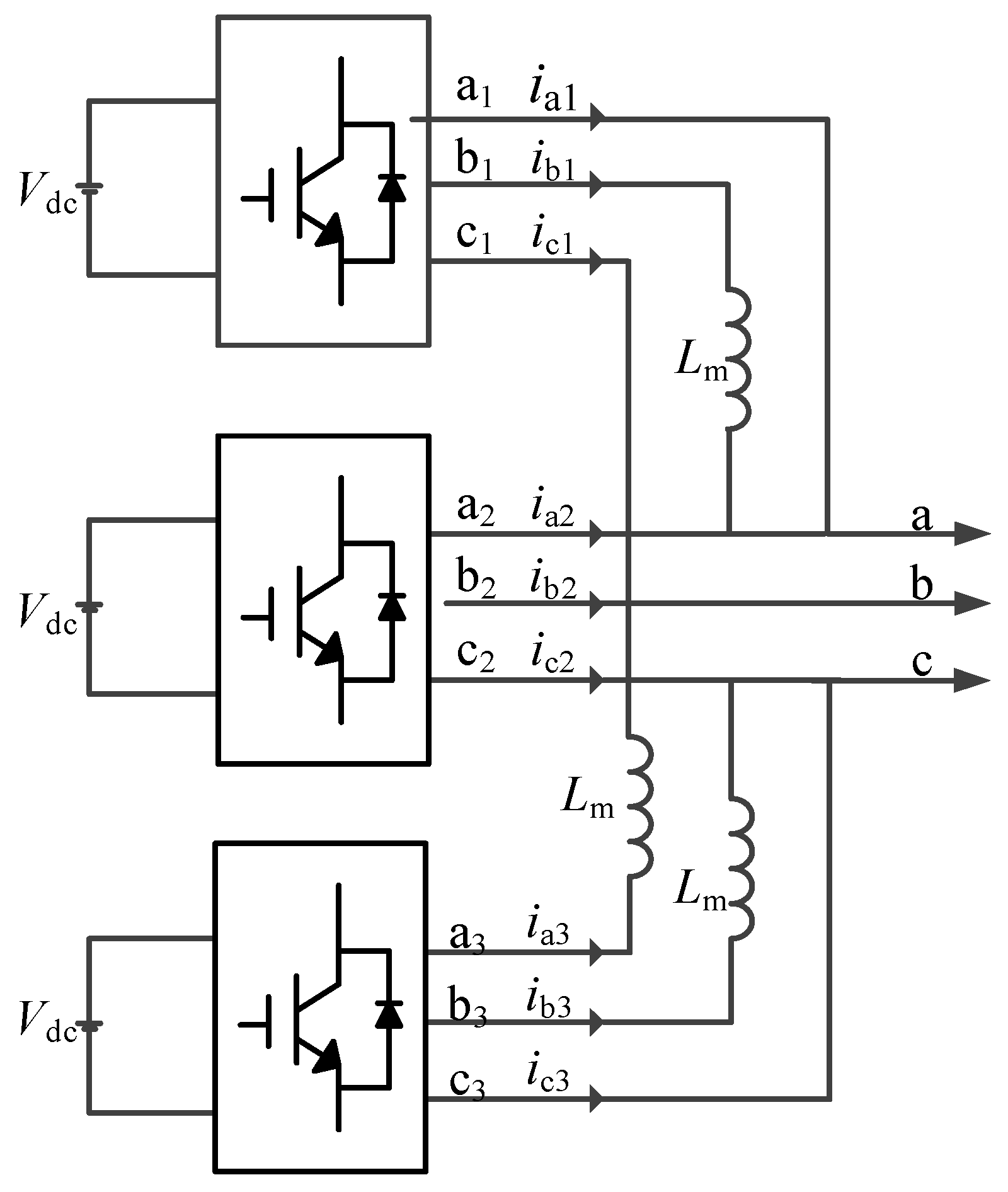
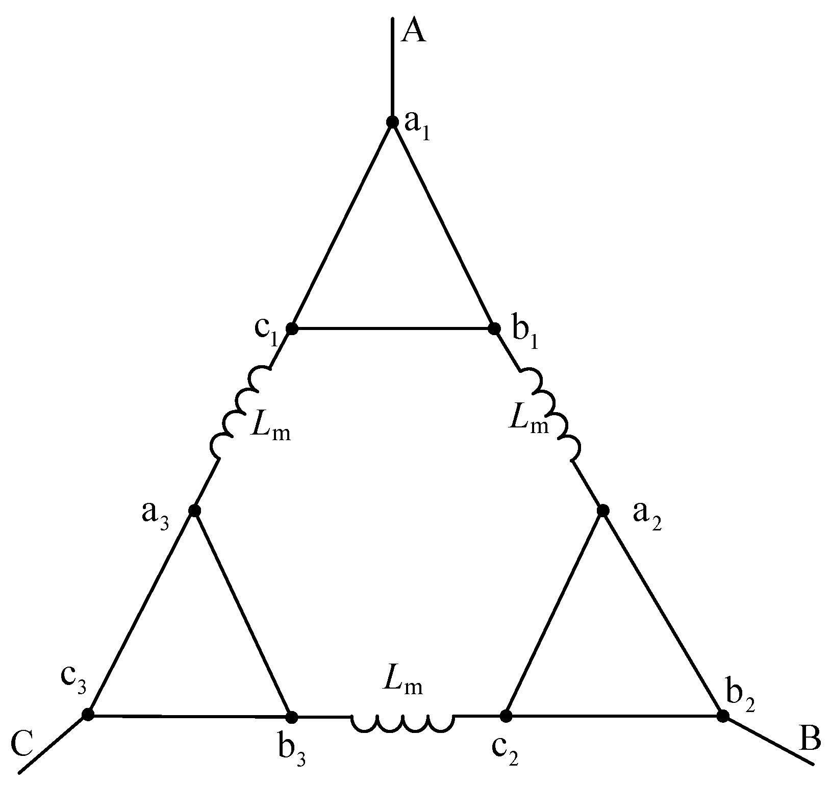
This study implements a multi-level C3PB configuration, deriving from conventional voltage-source inverter (VSI) principles to facilitate high-voltage grid interfacing through lower-rated semiconductors. Such a modular design is exceptionally beneficial for high-capacity renewable energy harvesting, as it minimizes component expenditures while reinforcing the stability of power conversion units tailored for electric mobility. The semiconductor arrangement is illustrated in Figure 1, which identifies nine distinct IGBT output clusters; for example, the primary module’s nodes are designated as $a_1,b_1$and $c_1$. The overarching operational logic of this cascaded structure is further detailed in the simplified representation in Figure 2.

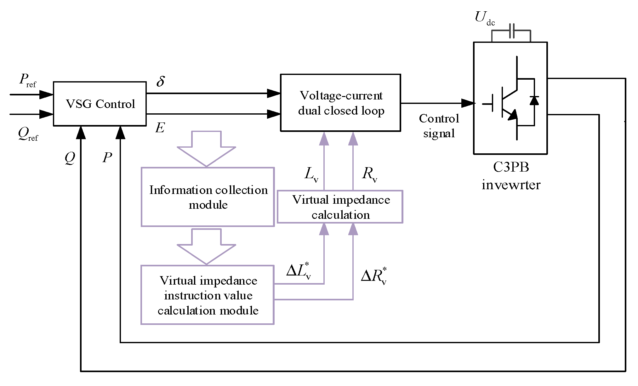
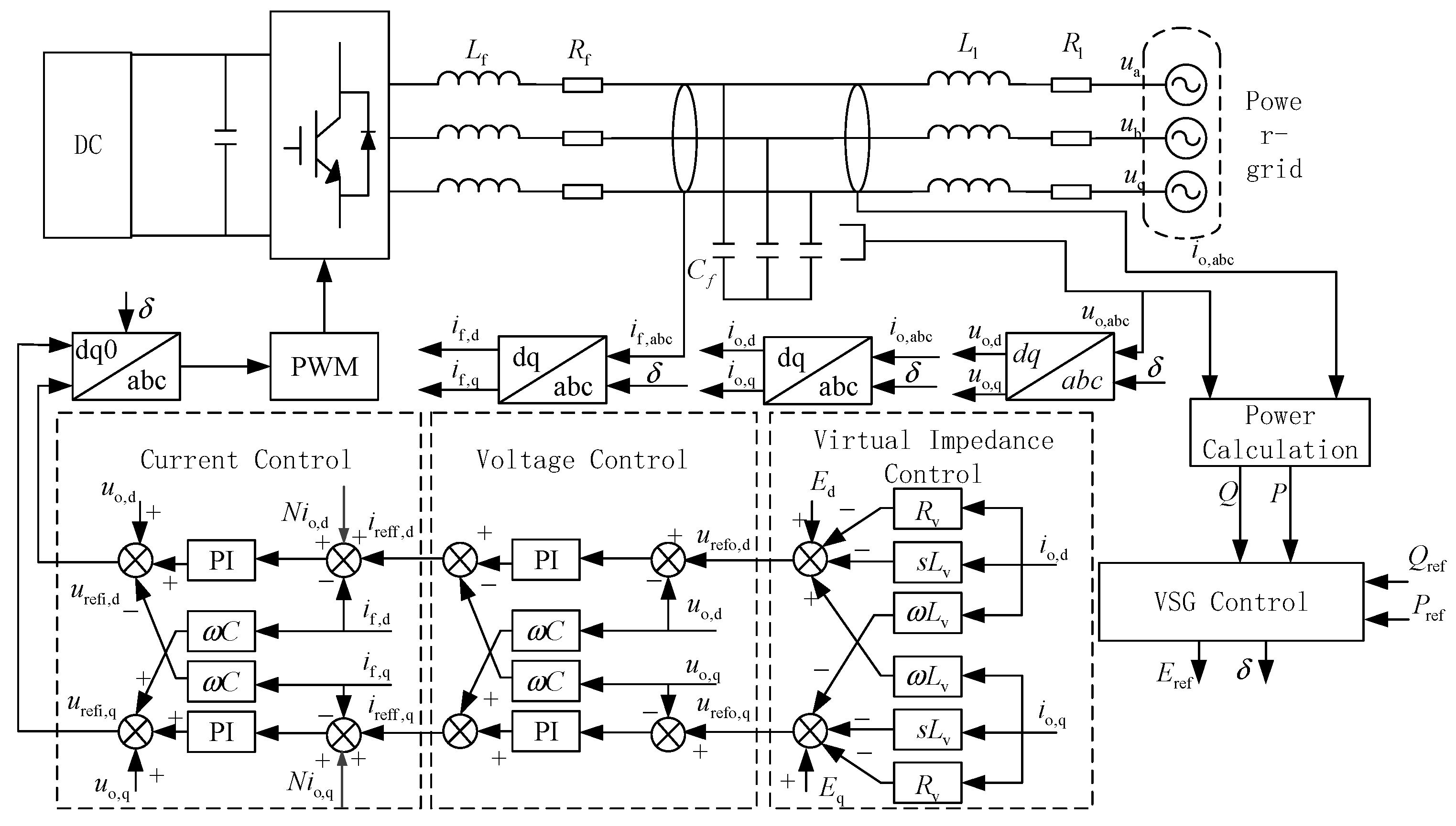
A pivotal advantage of the C3PB topology is its inherent fault-tolerant capability. As shown in Figure 2, the inverter can maintain continuous operation during a device failure by re-routing power through adjacent bridge arms. This structural redundancy is vital for enhancing the overall lifespan and reliability of the power electronics. Figure 3 maps the comprehensive system model under the VSG control paradigm, which synergizes four essential functional modules: the grid-tie hardware interface, the core VSG control logic, a hierarchical dual-loop voltage and current regulator, and the specialized virtual impedance decoupling mechanism. Detailed mathematical derivations for each functional block are elaborated in the following sections.

2.1. State-Space Representation of the Inverter Interface

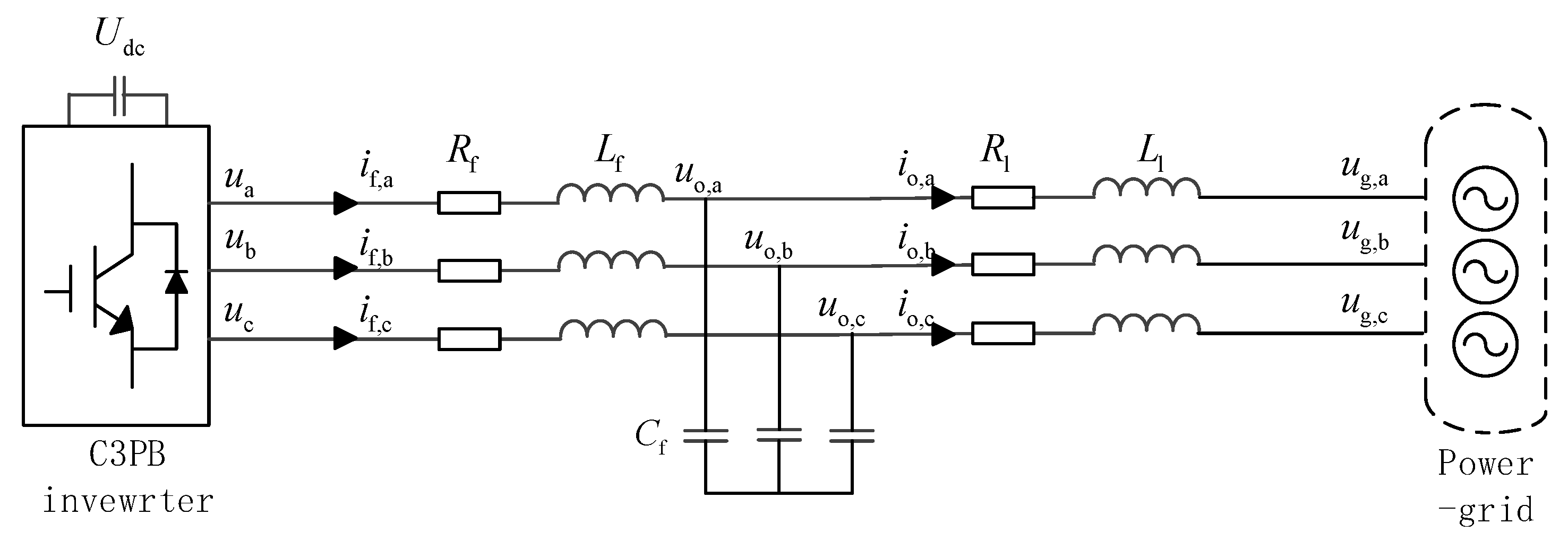
The hardware configuration visualized in Figure 4 incorporates an LC filter network coupled in parallel with the distribution grid. To simplify the subsequent control synthesis, the system’s mathematical model is projected from the fixed αβ coordinate system onto a synchronously rotating d−q reference frame. By applying this transformation, the transient voltage and current dynamics are governed by the following set of differential equations:

$$\left\{\begin{array}{l}{\displaystyle \frac{\mathrm{d}{u}_{\mathrm{o},\mathrm{d}}}{ \mathrm{d}t}}=\omega u_{\mathrm{o},\mathrm{q}}+{\displaystyle \frac{1}{C_{\mathrm{f}}}}{i}_{\mathrm{f},\mathrm{d}}-{\displaystyle \frac{1}{C_{\mathrm{f}}}}{i}_{\mathrm{o},\mathrm{d}}\\ {\displaystyle \frac{\mathrm{d}{u}_{\mathrm{o},\mathrm{q}}}{ \mathrm{d}t}}=-\omega u_{\mathrm{o},\mathrm{d}}+{\displaystyle \frac{1}{C_{\mathrm{f}}}}{i}_{\mathrm{f},\mathrm{q}}-{\displaystyle \frac{1}{C_{\mathrm{f}}}}{i}_{\mathrm{o},\mathrm{q}}\\ {\displaystyle \frac{\mathrm{d}{i}_{\mathrm{f},\mathrm{d}}}{ \mathrm{d}t}}=-{\displaystyle \frac{R_{\mathrm{f}}}{L_{\mathrm{f}}}}{i}_{\mathrm{f},\mathrm{d}}+\omega i_{\mathrm{f},\mathrm{q}}+{\displaystyle \frac{1}{L_{\mathrm{f}}}}{u}_{\mathrm{i},\mathrm{d}}-{\displaystyle \frac{1}{L_{\mathrm{f}}}}{u}_{\mathrm{o},\mathrm{d}}\\ {\displaystyle \frac{\mathrm{d}{i}_{\mathrm{f},\mathrm{q}}}{ \mathrm{d}t}}=-{\displaystyle \frac{R_{\mathrm{f}}}{L_{\mathrm{f}}}}{i}_{\mathrm{f},\mathrm{q}}-\omega i_{\mathrm{f},\mathrm{q}}+{\displaystyle \frac{1}{L_{\mathrm{f}}}}{u}_{\mathrm{i},\mathrm{q}}-{\displaystyle \frac{1}{L_{\mathrm{f}}}}{u}_{\mathrm{o},\mathrm{q}}\end{array}\right.$$

(1)

The d-axis and q-axis output voltages of the IGBT power stage, respectively; i_f,d and i_f,q stand for the d-axis and q-axis output currents of the IGBT power stage, respectively; u_o,d and u_o,q refer to the d-axis and q-axis output voltages after the LC filter, respectively; and i_o,d and i_o,q denote the d-axis and q-axis output currents after the LC filter, respectively.

2.2. Mathematical Model of VSG

The second-order virtual synchronous generator model emulates a conventional synchronous machine through an active-power–frequency droop that mimics the rotor swing equation: integrating the virtual torque imbalance yields the electrical angular velocity $\dot{\delta }$ and thus the phase δ. A reactive-power–voltage droop functions as an exciter, regulating the magnitude E of the virtual internal voltage. The combination of E and δ generates the reference voltage for inverter operation, endowing it with synthetic inertia, damping, and inherent frequency/voltage regulation—characteristics identical to those of a real synchronous generator.

The control architecture proposed herein utilizes a second-order representation designed to emulate the characteristic droop responses inherent in traditional synchronous units. This framework encapsulates both the frequency-active power (P − ω) and voltage-reactive power (Q − E) regulatory features of the VSG. Specifically, the mechanical swing dynamics governing the active power-frequency loop are expressed through the following differential relations:

$$\left\{\begin{array}{l}\dot{\delta }=\omega -{\omega }_{\mathrm{g}}\hfill \\ J\dot{\omega }={\displaystyle \frac{(P^{\ast }-P)-K_{\mathrm{p}}\left(\omega -{\omega }_0\right)}{{\omega }_0}}-D\left(\omega -{\omega }_0\right)\hfill \\ P={\displaystyle \frac{{\omega }_{\mathrm{c}}}{s+{\omega }_{\mathrm{c}}}}p\hfill \end{array}\right.$$

(2)

In Equation (2), the parameters $J$ and $D$ signify the virtual inertia constant and the damping coefficient, respectively. The cutoff bandwidth of the power filter is represented by ${\omega }_c$, whereas ${\omega }_0$ and ${\omega }_g$ correspond to the nominal and actual grid angular frequencies. Additionally, the variables $p$ and $P$ denote the active power signals before and after the low-pass filtering stage. The governing law for the VSG’s reactive power-voltage regulation is formulated as:

$$\left\{\begin{array}{l}E=U^{\ast }+K_{\mathrm{q}}\left(Q^{\ast }-Q\right)\hfill \\ Q={\displaystyle \frac{{\omega }_c}{s+{\omega }_c}}q\hfill \end{array}\right.$$

(3)

In the reactive power channel, q and Q denote the raw and smoothed power values, respectively.

2.3. Analytical Modeling of the Hierarchical Control Layers

To stabilize the energy conversion process, the VSG algorithm is typically embedded within a hierarchical voltage-current cascaded framework. Such an architecture facilitates high-fidelity regulation of the inverter’s output while reinforcing the overall system’s robustness. The linearized dynamics of the primary voltage regulation stage are defined as:

$$\left\{\begin{array}{l}{\displaystyle \frac{\mathrm{d}{\phi }_{\mathrm{d}}}{ \mathrm{d}t}}=u_{\mathrm{o},\mathrm{d}}^{\ast }-u_{\mathrm{o},\mathrm{d}}\hfill \\ i_{\mathrm{f},\mathrm{d}}^{\ast }=-\omega C_{\mathrm{f}}{u}_{\mathrm{o},\mathrm{q}}+k_{\mathrm{vP}}\left(u_{\mathrm{o},\mathrm{d}}^{\ast }-u_{\mathrm{o},\mathrm{d}}\right)+k_{\mathrm{vI}}{\phi }_{\mathrm{d}}+N{i}_{\mathrm{o},\mathrm{d}}\hfill \\ {\displaystyle \frac{\mathrm{d}{\phi }_{\mathrm{q}}}{ \mathrm{d}t}}=u_{\mathrm{o},\mathrm{q}}^{\ast }-u_{\mathrm{o},\mathrm{q}}\hfill \\ i_{\mathrm{f},\mathrm{q}}^{\ast }=\omega C_{\mathrm{f}}{u}_{\mathrm{o},\mathrm{d}}+k_{\mathrm{vP}}\left(u_{\mathrm{o},\mathrm{q}}^{\ast }-u_{\mathrm{o},\mathrm{q}}\right)+k_{\mathrm{vI}}{\phi }_{\mathrm{q}}+N{i}_{\mathrm{o},\mathrm{q}}\hfill \end{array}\right.$$

(4)

In this formulation, $u_{\mathrm{o}}^{\ast }$ signifies the target voltage setpoint, whereas $k_{vP}$ and $k_{vI}$ represent the proportional and integral regulatory gains of the outer-loop PI compensator.

Similarly, the differential equations characterizing the inner current regulation loop are expressed as follows:

$$\left\{\begin{array}{l}{\displaystyle \frac{\mathrm{d}{\lambda }_{\mathrm{d}}}{ \mathrm{d}t}}=i_{\mathrm{f},\mathrm{d}}^{\ast }-i_{\mathrm{f},\mathrm{d}}\hfill \\ u_{\mathrm{i},\mathrm{d}}^{\ast }=-\omega L_{\mathrm{f}}{i}_{\mathrm{f},\mathrm{q}}+k_{\mathrm{iP}}\left(i_{\mathrm{f},\mathrm{d}}^{\ast }-i_{\mathrm{f},\mathrm{d}}\right)+k_{\mathrm{iI}}{\lambda }_{\mathrm{d}}+u_{\mathrm{o},\mathrm{d}}\hfill \\ {\displaystyle \frac{\mathrm{d}{\lambda }_{\mathrm{q}}}{ \mathrm{d}t}}=i_{\mathrm{f},\mathrm{q}}^{\ast }-i_{\mathrm{f},\mathrm{q}}\hfill \\ u_{\mathrm{i},\mathrm{q}}^{\ast }=\omega L_{\mathrm{f}}{i}_{\mathrm{f},\mathrm{d}}+k_{\mathrm{iP}}\left(i_{\mathrm{f},\mathrm{q}}^{\ast }-i_{\mathrm{f},\mathrm{q}}\right)+k_{\mathrm{iI}}{\lambda }_{\mathrm{q}}+u_{\mathrm{o},\mathrm{q}}\hfill \end{array}\right.$$

(5)

where $\dot{\lambda }=i_{\mathrm{f}}^{\ast }-i_{\mathrm{f}}$, and i_f^* serves as the internal current reference command, with k_iP and k_if representing the corresponding proportional and integral gains for the current-loop PI controller. Furthermore, u_i^* denotes the derived modulation signal utilized for pulse-width modulation.

2.4. Mathematical Formulation of Adaptive Virtual Impedance

The integration of a virtual impedance loop substantially bolsters the regulatory efficacy of conventional droop mechanisms while improving load-sharing characteristics across the network. This control layer is mathematically characterized by the following set of differential equations:

$$\left\{\begin{array}{l}{L}_{\mathrm{v}}{\displaystyle \frac{d{i}_{\mathrm{o},\mathrm{d}}}{dt}}=-R_{\mathrm{v}}{i}_{\mathrm{o},\mathrm{d}}+L_{\mathrm{v}}\omega i_{\mathrm{o},\mathrm{q}}+E_{\mathrm{d}}-u_{\mathrm{o},\mathrm{d}}^{\ast }\hfill \\ L_{\mathrm{v}}{\displaystyle \frac{d{i}_{\mathrm{o},\mathrm{q}}}{dt}}=-R_{\mathrm{v}}{i}_{\mathrm{o},\mathrm{q}}-L_{\mathrm{v}}\omega i_{\mathrm{o},\mathrm{d}}+E_{\mathrm{q}}-u_{\mathrm{o},\mathrm{q}}^{\ast }\hfill \end{array}\right.$$

(6)

where L_v and R_v denote the virtual inductance and resistance, respectively.

An integrated analytical framework for the VSG control system is established by synthesizing the individual modules of the grid-interactive inverter, the VSG logic, the hierarchical dual-loop regulator, and the virtual impedance stage. This holistic representation encompasses the entirety of regulatory variables to provide a high-fidelity characterization of both transient and steady-state system behaviors. To facilitate small-signal stability analysis, the global non-linear state-space manifold is linearized around the equilibrium manifold (i_f,d0, i_f,q0, u_o,d0, u_o,q0, i_o,d0, i_o,q0, ω₀), yielding a comprehensive 14th-order model. This derived system consists of a sixth-order power stage, a fourth-order hierarchical controller, and a fourth-order active/reactive power loop. By designating the input perturbation vector as Δu = [U_g ω_g P^* Q^*]^T and the observed output as Δy = [P Q]^T, the linearized plant dynamics are mapped onto the state-space domain as follows:

$$\begin{array}{l}\Delta \dot{x}=A\Delta x+B\Delta u\\ \Delta y=C\Delta x\end{array}$$

(7)

where the state vector Δx and the corresponding system matrices A, B, and C are defined in a partitioned format:

$$\begin{array}{c}\Delta x={\left[\Delta \omega \Delta \delta \Delta P \Delta Q \Delta {\phi }_{\mathrm{d}} \Delta {\phi }_{\mathrm{q}} \Delta {\lambda }_{\mathrm{d}} \Delta {\lambda }_{\mathrm{q}} \Delta i_{\mathrm{f},\mathrm{d}} \Delta i_{\mathrm{f},\mathrm{q}} \Delta u_{\mathrm{o},\mathrm{d}} \Delta u_{\mathrm{o},\mathrm{q}} \Delta i_{\mathrm{o},\mathrm{d}} \Delta i_{\mathrm{o},\mathrm{q}}\right]}^{\mathrm{T}};\\ A=\left[\begin{array}{cccc}{A}_1& 0& 0& A_4\\ B_{11}{A}_2& 0& 0& B_3\\ C_{11}{C}_{12}{A}_2& C_{11}{C}_{21}& 0& C_{41}+C_{11}{C}_{42}\\ D_{11}(D_{12}{C}_{12}{A}_2+D_{14}{A}_2)+D_{15}{D}_{16}& D_{11}{D}_{12}{C}_{21}& D_{11}{D}_{31}& D_{41}{D}_{11}(D_{12}{C}_{12}{D}_{42})\end{array}\right];\\ B={\left[\begin{array}{cccc}{B}_1& B_{11}{B}_2& C_{11}{C}_{12}{B}_2& D_{11}{D}_{12}{C}_{12}{B}_2+D_{15}{B}_4\end{array}\right]}^{\mathrm{T}};\\ C={\left[\begin{array}{cccccccccccccc}0& 0& 1& 0& 0& 0& 0& 0& 0& 0& 0& 0& 0& 0\\ 0& 0& 0& 1& 0& 0& 0& 0& 0& 0& 0& 0& 0& 0\end{array}\right]}^{\mathrm{T}}.\end{array}$$

$$\begin{array}{l}{A}_1=\left[\begin{array}{cccc}{\displaystyle \frac{-D{\omega }_0-K_{\mathrm{p}}}{J{\omega }_0}}& 0& -{\displaystyle \frac{1}{J{\omega }_0}}& 0\\ 1& 0& 0& 0\\ 0& 0& -1& 0\\ 0& 0& 0& -1\end{array}\right];A_2=\left[\begin{array}{cccc}1& 0& 0& 0\\ 0& 0& 0& -K_{\mathrm{q}}\\ 0& 0& 0& 0\end{array}\right]\\ A_4=\left[\begin{array}{cccccc}0& 0& 0& 0& 0& 0\\ 0& 0& 0& 0& 0& 0\\ 0& 0& 1.5{\omega }_c{i}_{\mathrm{o},\mathrm{d}0}& 1.5{\omega }_c{i}_{\mathrm{o},\mathrm{q}0}& 1.5{\omega }_c{u}_{\mathrm{o},\mathrm{d}0}& 1.5{\omega }_c{u}_{\mathrm{o},\mathrm{q}0}\\ 0& 0& -1.5{\omega }_c{i}_{\mathrm{o},\mathrm{q}0}& 1.5{\omega }_c{i}_{\mathrm{o},\mathrm{d}0}& 1.5{\omega }_c{u}_{\mathrm{o},\mathrm{q}0}& -1.5{\omega }_c{u}_{\mathrm{o},\mathrm{d}0}\end{array}\right]\\ B_1=\left[\begin{array}{cccc}0& 0& {\displaystyle \frac{1}{J{\omega }_0}}& 0\\ -1& 0& 0& 0\\ 0& 0& 0& 0\\ 0& 0& 0& 0\end{array}\right];B_2=\left[\begin{array}{cccc}0& 0& 0& 0\\ 0& 0& 0& K_{\mathrm{q}}\\ 0& 0& 0& 0\end{array}\right]\\ B_3=\left[\begin{array}{cccc}0& \sin {\delta }_0& 0& 0\\ 0& \cos {\delta }_0& 0& 0\end{array}\right];B_4=\left[\begin{array}{cccccc}0& 0& -1& 0& 0& 0\\ 0& 0& 0& -1& 0& 0\end{array}\right];B_{11}=\left[\begin{array}{ccc}0& 1& 0\\ 0& 0& 1\end{array}\right]\\ C_{12}=\left[\begin{array}{ccc}-C_{\mathrm{f}}{u}_{\mathrm{o},\mathrm{q}0}& k_{\mathrm{vP}}& 0\\ C_{\mathrm{f}}{u}_{\mathrm{o},\mathrm{d}0}& 0& k_{\mathrm{vP}}\end{array}\right];C_{42}=\left[\begin{array}{cccccc}0& 0& -k_{\mathrm{vP}}& -{\omega }_0{C}_{\mathrm{f}}& N& 0\\ 0& 0& {\omega }_0{C}_{\mathrm{f}}& -k_{\mathrm{vP}}& 0& N\end{array}\right]\\ C_{11}=\left[\begin{array}{cc}1& 0\\ 0& 1\end{array}\right];C_{41}=\left[\begin{array}{cccccc}-1& 0& 0& 0& 0& 0\\ 0& -1& 0& 0& 0& 0\end{array}\right];C_{21}=\left[\begin{array}{cc}{k}_{\mathrm{vI}}& 0\\ 0& k_{\mathrm{vI}}\end{array}\right]\\ D_{31}=\left[\begin{array}{cc}{k}_{\mathrm{iI}}& 0\\ 0& k_{\mathrm{iI}}\end{array}\right];D_{12}=\left[\begin{array}{cc}{k}_{\mathrm{iP}}& 0\\ 0& k_{\mathrm{iP}}\end{array}\right];D_{14}=\left[\begin{array}{ccc}-L_{\mathrm{f}}{i}_{\mathrm{f},q0}& 0& 0\\ -L_{\mathrm{f}}{i}_{\mathrm{f},\mathrm{d}0}& 0& 0\end{array}\right]\\ D_{16}=\left[\begin{array}{cccc}0& U_{\mathrm{g}0}\cos {\delta }_0& 0& 0\\ 0& -U_{\mathrm{g}0}\sin {\delta }_0& 0& 0\end{array}\right];D_{42}=\left[\begin{array}{cccccc}-k_{\mathrm{iP}}& -{\omega }_0{L}_{\mathrm{f}}& 0& 0& 0& 0\\ {\omega }_0{L}_{\mathrm{f}}& -k_{\mathrm{iP}}& 0& 0& 0& 0\end{array}\right]\\ D_{41}=\left[\begin{array}{cccccc}-{\displaystyle \frac{R_{\mathrm{f}}}{L_{\mathrm{f}}}}& {\omega }_0& -{\displaystyle \frac{1}{L_{\mathrm{f}}}}& 0& 0& 0\\ -{\omega }_0& -{\displaystyle \frac{R_{\mathrm{f}}}{L_{\mathrm{f}}}}& 0& -{\displaystyle \frac{1}{L_{\mathrm{f}}}}& 0& 0\\ {\displaystyle \frac{1}{C_{\mathrm{f}}}}& 0& 0& {\omega }_0& -{\displaystyle \frac{1}{C_{\mathrm{f}}}}& 0\\ 0& {\displaystyle \frac{1}{C_{\mathrm{f}}}}& -{\omega }_0& 0& 0& -{\displaystyle \frac{1}{C_{\mathrm{f}}}}\\ 0& 0& {\displaystyle \frac{1}{L_{\mathrm{l}}}}& 0& -{\displaystyle \frac{R_{\mathrm{l}}}{L_{\mathrm{l}}}}& {\omega }_0\\ 0& 0& 0& {\displaystyle \frac{1}{L_{\mathrm{l}}}}& -{\omega }_0& -{\displaystyle \frac{R_{\mathrm{l}}}{L_{\mathrm{l}}}}\end{array}\right];D_{11}=\left[\begin{array}{cc}{\displaystyle \frac{1}{L_{\mathrm{f}}}}& 0\\ 0& {\displaystyle \frac{1}{L_{\mathrm{f}}}}\\ 0& 0\\ 0& 0\\ 0& 0\\ 0& 0\end{array}\right];D_{15}=\left[\begin{array}{cc}0& 0\\ 0& 0\\ 0& 0\\ 0& 0\\ -{\displaystyle \frac{1}{L_{\mathrm{l}}}}& 0\\ 0& -{\displaystyle \frac{1}{L_{\mathrm{l}}}}\end{array}\right]\end{array}$$

3. Implementing Adaptive Virtual Impedance Decoupling via a Refined 5th-Order Analytical Framework

3.1. Theoretical Foundation of the 5th-Order Electromagnetic Formulation

While the full-order model of a VSG-controlled inverter provides a precise representation of both transient and steady-state responses, its high dimensionality leads to a substantial computational load and extended runtime. This complexity also hinders intuitive understanding and complicates stability analysis. Meanwhile, the conventional third-order model is only valid for high-inertia, high-damping scenarios and cannot reflect the stability characteristics of low-inertia, weakly damped systems.

Grounded in the preceding comprehensive analysis, a 5th-order electromagnetic-dynamic representation is formulated, specifically integrating the electromagnetic transients of the transmission network. By merging a 3rd-order power regulation stage with a 2nd-order stage for output power, the model effectively recreates system-wide stability. More importantly, it facilitates the precise observation of the three major low-frequency poles as operational settings fluctuate. While the “inverter time scale” currently lacks a rigid definition, examining the distribution of characteristic roots within the complete model highlights specific zones of high parameter sensitivity. Specifically, high-frequency feature roots are primarily dictated by the hardware interface—namely the LC filter and transmission line parameters—alongside the operating voltage and current levels. Conversely, low-frequency poles remain highly sensitive to the dynamics of the power loop. To account for the dynamic interactions within the cabling, three-phase sinusoidal components are represented as time-dependent vectors:

$$P(x(t))={\displaystyle \frac{dX(t)}{dt}}=X(t)e^{\mathrm{j}\delta (t)}$$

(8)

Within this analytical framework, P is the projection operator for the non-stationary vector, where $X(t)$ represents the signal amplitude, and δ(t) is the initial phase angle. The term $\dot{X}(t)$ refers to the time-varying vector representation.

Differentiating $x(t)$ with respect to time yields:

$$P\left({\displaystyle \frac{d}{dt}}x(t)\right)={\displaystyle \frac{d}{dt}}({\displaystyle \frac{dX(t)}{dt}})+\mathrm{j}\omega {\displaystyle \frac{dX(t)}{dt}}$$

(9)

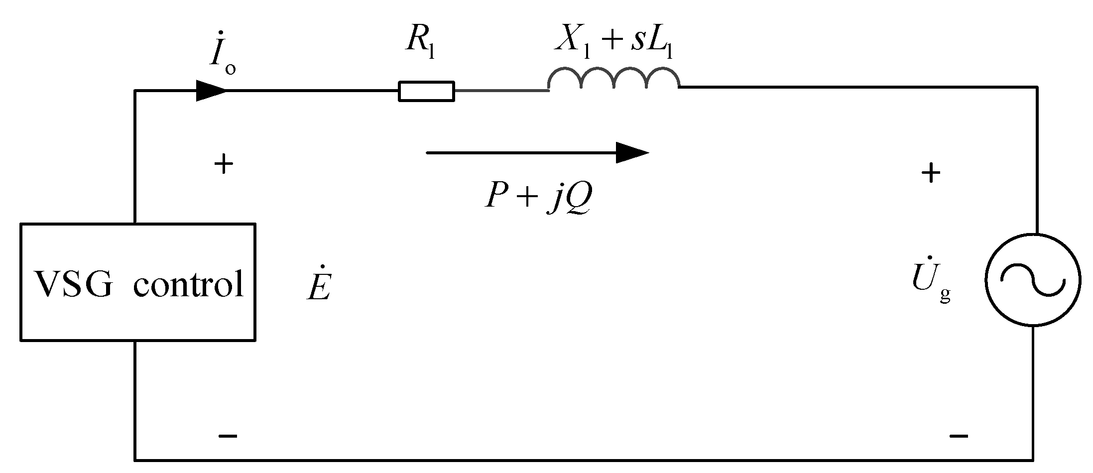
Conventional “quasi-steady-state” third-order models typically neglect the dynamic term $d\dot{X}(t)/dt$. However, overlooking transient variations in amplitude, frequency, and phase angle during dynamic events can obscure critical stability factors. Therefore, incorporating these transient effects is essential. The resulting circuit topology, adjusted for these dynamics, is depicted in Figure 5.

To precisely reflect these rapid temporal shifts, the mathematical expression governing the inverter’s terminal current is reformulated as:

$${\dot{I}}_{\mathrm{o}}={\displaystyle \frac{1}{R_{\mathrm{l}}+\mathrm{j}{X}_{\mathrm{l}}+s{L}_{\mathrm{l}}}}(E\angle \delta -U_{\mathrm{g}}\angle 0)$$

(10)

Accordingly, the equations governing the system’s active and reactive power are reformulated as:

$$\left\{\begin{array}{l}P={\displaystyle \frac{\left(R_{\mathrm{l}}+s{L}_{\mathrm{l}}\right)\left(E^2-E{U}_{\mathrm{l}}\cos \delta \right)+X_{\mathrm{l}}E{U}_{\mathrm{l}}\sin \delta }{{\left(R_{\mathrm{l}}+s{L}_{\mathrm{l}}\right)}^2+X_{\mathrm{l}}^2}}\\ Q={\displaystyle \frac{X_{\mathrm{l}}\left(E^2-E{U}_{\mathrm{g}}\cos \delta \right)-\left(R_{\mathrm{l}}+s{L}_{\mathrm{l}}\right)E{U}_{\mathrm{g}}\sin \delta }{{\left(R_{\mathrm{l}}+s{L}_{\mathrm{l}}\right)}^2+X_{\mathrm{l}}^2}}\end{array}\right.$$

(11)

In the neighborhood of the steady-state operating point, small deviations of state variables are much smaller than their steady-state values, allowing nonlinear terms to be neglected. The linearized model thus accurately captures low-frequency dynamics and stability characteristics. Linearization at the steady-state operating point (E₀, U_g0, δ₀) therefore yields:

$$\left[\begin{array}{c}\Delta \dot{\delta }\\ \Delta \dot{\omega }\\ \Delta \dot{Q}\end{array}\right]=\left[\begin{array}{ccc}0& 1& 0\\ 0& {\displaystyle \frac{-D{\omega }_0-K_p}{J{\omega }_0}}& 0\\ 0& 0& -{\omega }_c\end{array}\right]\left[\begin{array}{c}\Delta \delta \\ \Delta \omega \\ \Delta Q\end{array}\right]+\left[\begin{array}{ccc}-1& 0& 0\\ 0& {\displaystyle \frac{-1}{J{\omega }_0}}& {\displaystyle \frac{1}{J{\omega }_0}}\\ 0& 0& {\omega }_c\end{array}\right]\left[\begin{array}{c}\Delta {\omega }_g\\ \Delta P\\ \Delta Q_{ref}\end{array}\right]$$

(12)

$$\left[\begin{array}{c}\Delta P\\ \Delta Q\\ \Delta E\end{array}\right]=\left[\begin{array}{ccc}{G}_{P-\delta }& 0& G_{P-E}\\ G_{Q-\delta }& 0& G_{Q-E}\\ 0& -K_q& 0\end{array}\right]\left[\begin{array}{c}\Delta \delta \\ \Delta Q\\ \Delta E\end{array}\right]+\left[\begin{array}{cc}{G}_{P-g}& 0\\ G_{Q-g}& 0\\ 0& K_q\end{array}\right]\left[\begin{array}{c}\Delta U_g\\ \Delta Q_{ref}\end{array}\right]$$

(13)

where

$$\left\{\begin{array}{l}{G}_{\mathrm{P}-\mathrm{E}}(s)={\displaystyle \frac{\left(s{L}_{\mathrm{l}}+R_{\mathrm{l}}\right)\left(2E_0-U_{\mathrm{g}0}\cos {\delta }_0\right)+X_{\mathrm{l}}{U}_{\mathrm{g}0}\sin {\delta }_0}{{\left(s{L}_{\mathrm{l}}+R_{\mathrm{l}}\right)}^2+X_{\mathrm{l}}^2}}\hfill \\ G_{\mathrm{P}-\mathsf{\delta }}(s)={\displaystyle \frac{\left(s{L}_{\mathrm{l}}+R_{\mathrm{l}}\right)E_0{U}_{\mathrm{g}0}\sin {\delta }_0+X_{\mathrm{l}}{E}_0{U}_{\mathrm{g}0}\cos {\delta }_0}{{\left(s{L}_{\mathrm{l}}+R_{\mathrm{l}}\right)}^2+X_{\mathrm{l}}^2}}\hfill \\ G_{\mathrm{P}-\mathrm{g}}(s)={\displaystyle \frac{-\left(s{L}_{\mathrm{l}}+R_{\mathrm{l}}\right)E_0\cos {\delta }_0+X_{\mathrm{l}}{E}_0\sin {\delta }_0}{{\left(s{L}_{\mathrm{l}}+R_{\mathrm{l}}\right)}^2+X_{\mathrm{l}}^2}}\hfill \\ G_{\mathrm{Q}-\mathrm{E}}(s)={\displaystyle \frac{X_{\mathrm{l}}\left(2E_0-U_{\mathrm{g}0}\cos {\delta }_0\right)-\left(s{L}_{\mathrm{l}}+R_{\mathrm{l}}\right)U_{\mathrm{g}0}\sin {\delta }_0}{{\left(s{L}_{\mathrm{l}}+R_{\mathrm{l}}\right)}^2+X_{\mathrm{l}}^2}}\hfill \\ G_{\mathrm{Q}-\mathsf{\delta }}(s)={\displaystyle \frac{X_{\mathrm{l}}{E}_0{U}_{\mathrm{g}0}\sin {\delta }_0-\left(s{L}_{\mathrm{l}}+R_{\mathrm{l}}\right)E_0{U}_{\mathrm{g}0}\cos {\delta }_0}{{\left(s{L}_{\mathrm{l}}+R_{\mathrm{l}}\right)}^2+X_{\mathrm{l}}^2}}\hfill \\ G_{\mathrm{Q}-\mathrm{g}}(s)={\displaystyle \frac{-X_{\mathrm{l}}{E}_0\cos {\delta }_0-\left(s{L}_{\mathrm{l}}+R_{\mathrm{l}}\right)E_0\sin {\delta }_0}{{\left(s{L}_{\mathrm{l}}+R_{\mathrm{l}}\right)}^2+X_{\mathrm{l}}^2}}\hfill \end{array}\right.$$

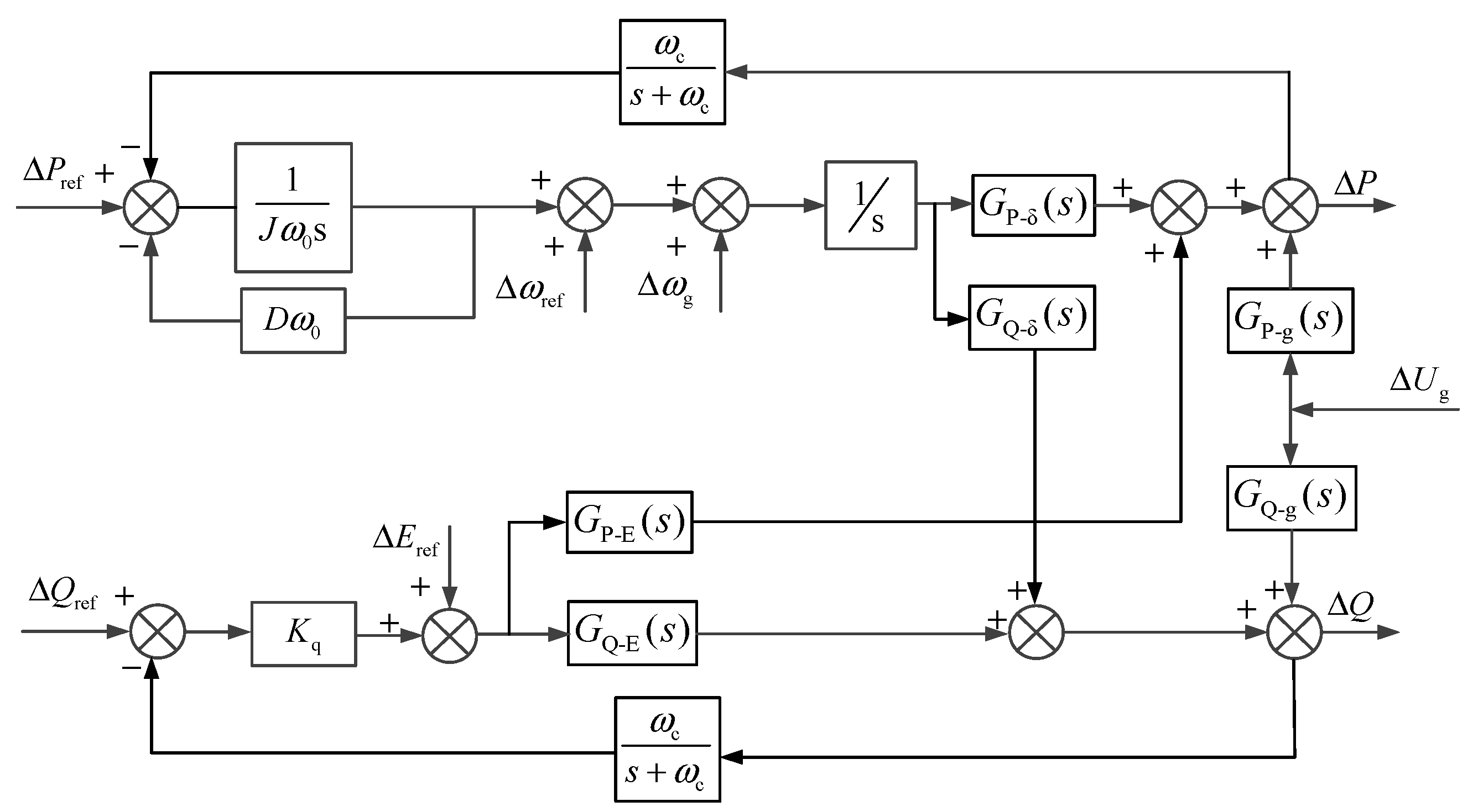
Guided by the preceding mathematical synthesis, the integrated state-space architecture of the VSG control scheme is synthesized, as visualized in the block diagram of Figure 6. This formulation illustrates that the proposed 5th-order framework bifurcates into two coupled layers: a 3rd-order power-frequency regulation stage interconnected with a 2nd-order reactive-voltage subsystem. This hierarchical arrangement ensures a high-fidelity representation of the complex interactions between the real and imaginary power channels.

3.2. Dynamic Decoupling Logic Grounded in the High-Fidelity 5th-Order Framework

Traditional methods for adaptive virtual impedance decoupling typically rely on quasi-steady-state assumptions, often neglecting inherent system dynamics. In contrast, the adaptive dynamic virtual impedance algorithm proposed herein explicitly addresses these dynamics, effectively resolving cross-coupling between active and reactive power loops while significantly enhancing overall dynamic performance.

Observations from Figure 6 suggest that while virtual admittance modulation allows for the synthesis of purely reactive line characteristics, a persistent interdependence exists between active/reactive power fluctuations and the internal angle. This interaction is further exacerbated as the phase displacement increases. In realistic operating environments, the power angle undergoes dynamic shifts driven by the active power throughput of the inverter, thereby complicating the decoupling objectives. Furthermore, owing to the disparate time constants inherent in converter control hierarchies, the VSG framework—though providing synthetic inertia and damping—exhibits a response latency that falls short of the rapid timescales achieved by standard feed-forward decoupled cascaded loops.

To address these challenges, the current study proposes a self-tuning virtual impedance decoupling architecture designed to isolate the regulatory interactions between real and imaginary power flows. By effectively partitioning the control loops within the VSG framework, this method suppresses the undesirable sensitivity of reactive power to angular fluctuations, thereby ensuring superior precision in steady-state operation. Moreover, the proposed control logic significantly bolsters the system’s robustness and transient regulatory performance when operating under adverse scenarios, such as high-impedance networks, expansive power angles, or weak-grid environments.

Figure 7 depicts the simplified circuit configuration of the grid-connected VSG under the influence of virtual impedance. The resultant transmission impedance, defined as Z_eq, is the aggregate of the intrinsic line parameters and the synthesized virtual components:

$$Z_{\mathrm{eq}}=\left(R_{\mathrm{l}}+R_{\mathrm{v}}\right)+\mathrm{j}\omega \left(L_{\mathrm{l}}+L_{\mathrm{v}}\right)=R_{e\mathrm{q}}+\mathrm{j}{X}_{\mathrm{eq}}$$

(14)

The cross-coupling phenomenon primarily stems from how power angle perturbations, Δδ, impact the reactive power output. Although modifying the impedance angle θ offers a mechanism to offset Δδ, any adjustment to θ inevitably disturbs the reactive power amplitude Q. Consequently, a corrective tuning of the virtual impedance is mandatory to eliminate such unintended coupling.

To evaluate the linear sensitivity of reactive power fluctuations, the linearized relationship mapping the deviations in $\theta$ and $\delta$ is established through the following expression:

$$\Delta Q=G_{Q\theta }\Delta \theta +G_{Q\delta }\Delta \delta$$

(15)

$$\left\{\begin{array}{l}{G}_{Q\theta }={\displaystyle \frac{U_g}{Z_{eq}}}\left[U_0\cos ({\theta }_0-{\delta }_0)-U_g\cos {\theta }_0\right]\hfill \\ G_{Q\delta }=-{\displaystyle \frac{U_g{U}_0}{Z_{eq}}}\cos ({\theta }_0-{\delta }_0)\hfill \end{array}\right.$$

(16)

In this formulation, ${ \theta }_0$ signifies the equilibrium impedance angle. The total variation in the impedance angle is decomposed into a dual-functional structure: $\mathsf{\Delta }{\delta }^{*}$ serves to counteract the reactive power perturbations cross-coupled from the power angle, while $\mathsf{\Delta }{\theta }^{*}$ is specifically designed for addressing the self-induced deviations within the reactive power channel itself.

$$\left\{\begin{array}{l}\Delta \theta =\Delta {\delta }^{\ast }+\Delta {\theta }^{\ast }\hfill \\ \Delta {\delta }^{\ast }=\Delta \delta \hfill \end{array}\right.$$

(17)

Since the compensation aims to nullify reactive power fluctuations, it follows that:

$$\Delta Q=G_{Q\theta }\Delta {\theta }^{\ast }-G_{Q\delta }(\Delta {\delta }^{\ast }+\Delta {\theta }^{\ast })=0$$

(18)

Solving this nullification condition allows for the derivation of the feed-forward compensation gain:

$$\Delta {\theta }^{\ast }={\displaystyle \frac{G_{Q\delta }}{G_{Q\theta }-G_{Q\delta }}}\Delta {\delta }^{\ast }=K_{const}\Delta {\delta }^{\ast }$$

(19)

In this context, the scalar $K_{const}$ represents a decoupling coefficient fundamentally dictated by the system’s steady-state equilibrium parameters ($E_0,U_{g0},{\theta }_0,{\delta }_0$). Consequently, by consolidating the incremental relationships, the total compensatory adjustment for the impedance angle is established as:

$$\Delta \theta =\left(1+K_{\mathrm{const} }\right)\Delta \delta$$

(20)

The proposed strategy maintains a constant modulus for the equivalent impedance. During large virtual impedance adjustments, ensuring a constant impedance modulus is crucial to prevent persistent voltage fluctuations. Consequently:

$$\left\{\begin{array}{l}|\Delta Z|={\left(R_{\mathrm{eq}0}^2+X_{\mathrm{eq}0}^2\right)}^{-{\displaystyle \frac{1}{2}}}\left(R_{\mathrm{eq}0}\Delta R+X_{\mathrm{eq}0}\Delta X\right)=0\\ \Delta \theta ={\displaystyle \frac{1}{Z_{\mathrm{eq}0}^2}}\left(R_{\mathrm{eq}0}\Delta X-X_{\mathrm{eq}0}\Delta R\right)\end{array}\right.$$

(21)

The steady-state parameters $R_{eq0}$, $X_{eq0}$ and $Z_{eq0}$ serve as benchmark resistance, reactance, and total impedance, respectively, chosen to ensure the magnitude of $Z_{eq0}$ remains invariant. The incremental deviations $\mathsf{\Delta }R$, $\mathsf{\Delta }X$ and $\mathsf{\Delta }Z$ account for the fluctuations within these respective domains. To suppress reactive oscillations triggered by angular shifts, the compensatory reactance is dynamically recalibrated. The corrective mapping between the angular perturbation and the impedance adjustments is formulated in vector-matrix notation as:

$$\left[\begin{array}{c}\Delta R\\ \Delta X\end{array}\right]=\left[\begin{array}{c}-X_0\\ R_0\end{array}\right](1+K_{const})\Delta \delta$$

(22)

Given that the physical grid and feeder parameters are relatively static, the operational adjustments are restricted solely to the virtual impedance components. Thus, within the framework of the proposed control strategy, $\mathsf{\Delta }R$ and $\mathsf{\Delta }X$ specifically represent the adaptive tuning of the virtual resistance and reactance within the $Z_v$ controller to satisfy the stabilization requirements.

Within this self-adaptive decoupling framework, the virtual impedance parameters are dynamically modulated by the system’s angular evolution, which necessitates a high-precision estimation of the power angle. To alleviate the numerical burden without sacrificing regulatory fidelity, the angular deviation is estimated through a neighborhood linear expansion of the system model in the vicinity of the quiescent equilibrium:

$$\Delta \delta =K_1(P-P_{ref})$$

(23)

In this context, $K_1$ signifies the sensitivity gain of the power angle relative to active power, which is evaluated as:

$$K_1^{-1}=D_{\delta }+D_{\theta }\Delta \theta$$

(24)

where $D_{\delta }$ characterizes the first-order sensitivity of power to the angle, and $D_{\theta }$ serves as a second-order correction term derived from the impedance-angle gradient:

$$D_{\theta }={\left.{\displaystyle \frac{\partial D_{\delta }}{\partial \theta }}\right|}_{({\theta }_0,{\delta }_0)}={\displaystyle \frac{U_g{U}_o}{Z_{eq0}}}\cos ({\theta }_0-{\delta }_0)$$

(25)

Figure 8 illustrates the conceptual flowchart of the proposed self-tuning impedance mechanism, anchored in the high-fidelity electromagnetic model. The operational sequence involves acquiring the baseline equilibrium, executing real-time perturbation calculations, and updating the virtual impedance commands to achieve precise decoupling.

First, the steady-state voltage, power angle, and virtual-impedance baseline are acquired, and real-time deviations are calculated online.

Second, dynamic corrections R_v and L_v are recalculated at each sampling instant to update the impedance command.

Third, these corrections are fed into the dual-loop controller to generate PWM signals for the IGBTs, thereby achieving adaptive decoupling.

4. Simulation and Experimental Results

To assess the regulatory performance and decoupling efficacy of the proposed dynamic self-tuning strategy, a comprehensive grid-interactive VSG testbed was developed within the PSCAD/EMTDC software environment (version 5.0). This high-fidelity simulation setup facilitates a rigorous comparison under various disturbance scenarios. The critical physical constants and control coefficients utilized for this numerical verification are summarized in

Table 1. Key parameters used in the VSG system simulation.

Parameter	Value	Unit
Rated power (Pn)	50	kW
Rated voltage (Vrms)	220	V
Rated frequency (f0)	50	Hz
DC voltage (Vdc)	800	V
PWM frequency (fsw)	12,800	Hz
Filter inductor (Lf)	1.35	mH
Filter capacitor (Cf)	50	μF
Filter resistor (Rf)	0.01	Ω
Line resistance (Rline)	0.5	Ω
Line inductor (Lline)	2	mH

.

4.1. Response to Step Changes in Active Power

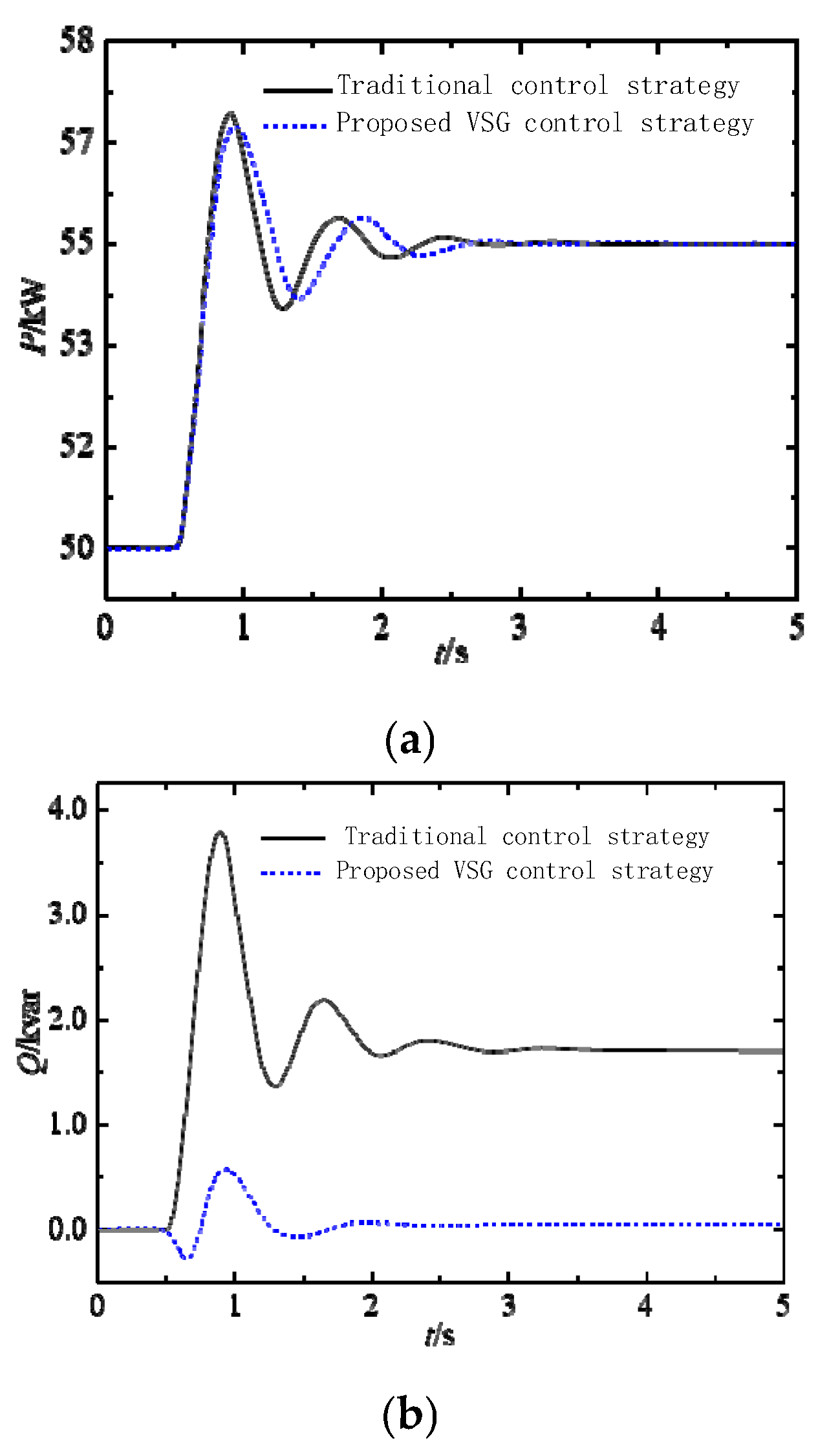
Initially, the VSG system delivers 50 kW of active power and 0 kvar of reactive power to the grid. The system reaches steady state at a power angle of δ₀ = 0.6, with a line impedance ratio set to R₁/X₁ = 0.4. These simulation conditions represent a high impedance ratio and large power angle scenario, where severe coupling is expected.

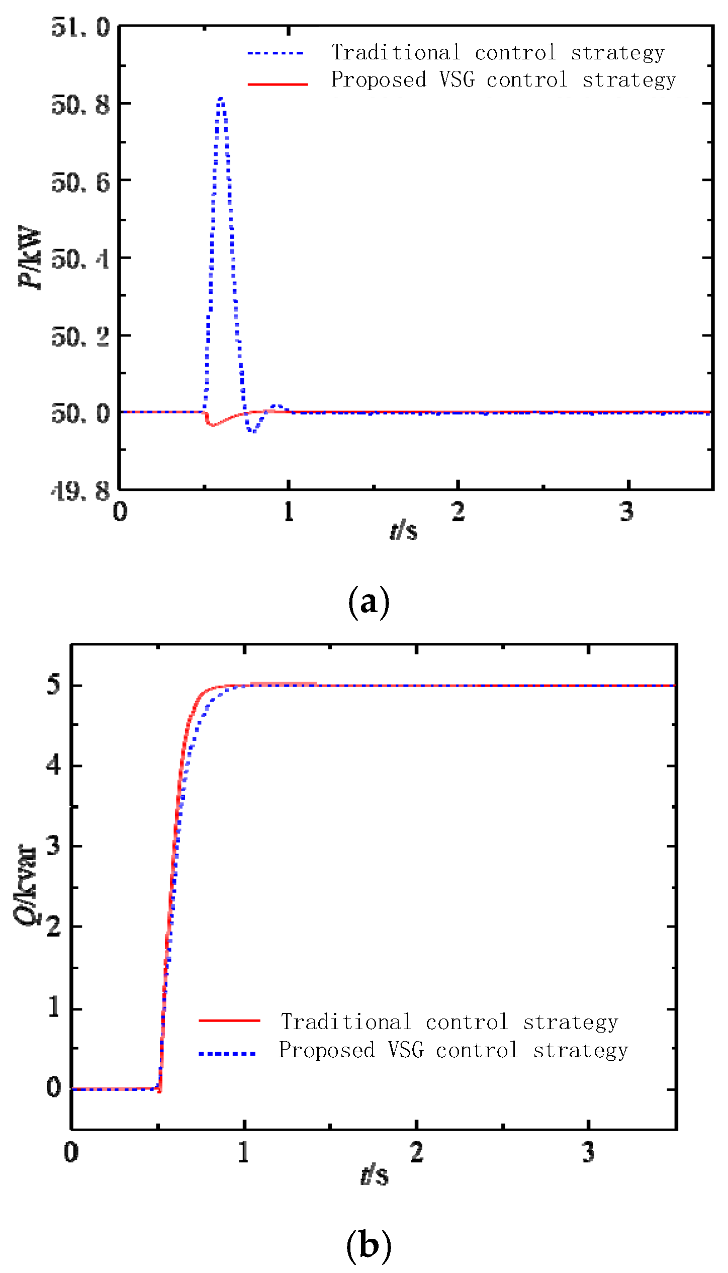
A sudden load increment of $\mathsf{\Delta }P=5 \mathrm{k}\mathrm{W}$ is applied at the $0.5 \mathrm{s}$ mark to evaluate the system’s regulatory resilience. The resulting performance metrics for the C3PB-based inverter, contrasting the legacy control framework with the introduced self-adaptive impedance compensation, are visualized in Figure 9. In particular, the transient evolution of the real and imaginary power components is detailed in subplots (a) and (b), respectively.

Analysis of Figure 9 highlights a pronounced interaction between the real and imaginary power channels under the legacy control framework, symptomatic of insufficient system damping. Upon the occurrence of the real-power step, the reactive component undergoes a substantial peak excursion, with the maximum transient deviation climbing to 3.82 kvar. Furthermore, as the system settles, the lack of compensation allows the angular shift to permanently bias the reactive equilibrium, resulting in a steady-state error where the output drifts from its 0 var reference to 1.71 kvar.

In contrast, the implementation of the recommended self-adaptive decoupling logic successfully isolates the two power channels. The simulation data confirms that the reactive power baseline remains immune to fluctuations in the real power throughput, accurately returning to its pre-disturbance setpoint. This enhanced performance verifies that the proposed strategy eliminates the structural dependency between real and imaginary power. By significantly reinforcing the inverter system’s damping ratio, the new control logic ensures superior dynamic resilience. Comparative benchmarks reveal that, relative to the legacy approach, the proposed methodology curtails the peak overshoot by 85.6% and accelerates the stabilization process by 42%, thereby achieving a higher standard of grid-tie stability and regulatory precision.

4.2. Sudden Change in Reactive Power

At the onset of the test, the VSG framework sustains a baseline output of 50 kW real power while maintaining a zero imaginary power profile. To evaluate the decoupling efficacy, a reactive load impulse of $\mathsf{\Delta }Q=5$ kvar is initiated at the 0.5 s mark. Figure 10 presents a comparative performance evaluation of the C3PB inverter under the legacy control versus the suggested adaptive impedance logic. The resulting fluctuations in the real and imaginary power channels are detailed in subplots (a) and (b), providing a clear contrast in their regulatory stability.

The quantitative performance metrics derived from Figure 10 indicate that, in the absence of decoupling logic, the real-power injection is significantly disrupted by reactive-power fluctuations. Specifically, the sudden reactive step triggers a substantial transient swing in the real power channel, reaching a peak deviation of 0.83 kW. Although the inherent integral-based secondary control within the VSG enables the real power to eventually return to its 50 kW setpoint, the recovery is notably sluggish, requiring a settling period of 1.39 s.

Conversely, the integration of the recommended self-adaptive impedance compensation fundamentally redefines the transient trajectory. The cross-talk between the power loops is effectively suppressed, with the maximum real-power perturbation curtailed to a negligible −0.03 kW. Furthermore, the stabilization process is markedly accelerated, with the total regulation time dropping to just 0.69 s. This stark contrast validates the operational superiority of the proposed strategy, demonstrating its ability to isolate the real and imaginary power channels and maintain high-fidelity tracking during rapid load transitions.

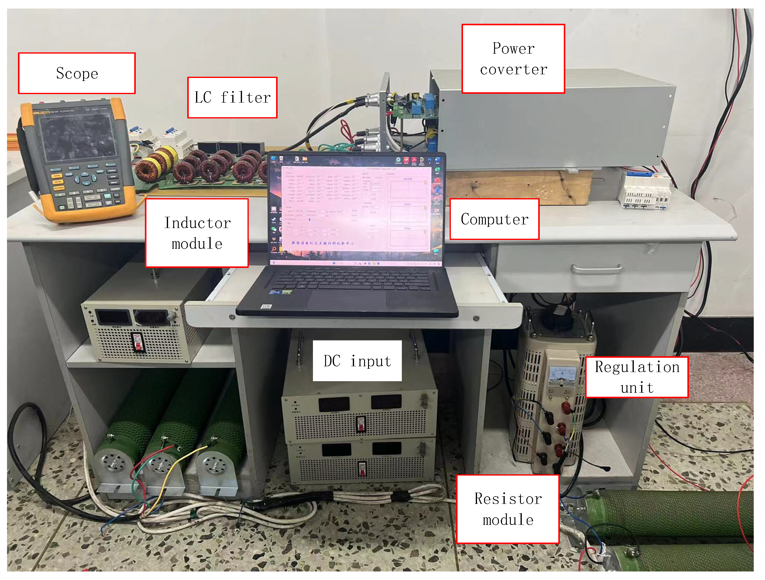
For empirical confirmation of the recommended control efficacy, a physical testbed centered on the two-stage C3PB topology was assembled. The laboratory configuration, detailed in Figure 11, integrates a primary voltage supply, a high-voltage three-phase bridge network, an impedance-matched load emulator, and a supervisory workstation for digital signal processing. Detailed operational constants for this hardware prototype are cataloged in

Table 2. Hardware Configuration and Control Coefficients for the C3PB Prototype.

Parameter	Value	Unit
DC voltage (Vdc)	800	V
RMS Grid-Side Phase Voltage (Vg)	220	V
Rated frequency (f)	50	Hz
Filter inductance (L)	6	mH
Filter capacitor (C)	5	uF
Feeder Equivalent Resistance (Rline)	0.5	Ω
Feeder Equivalent Inductance (Lline)	1	mH
Inertia (J)	0.8	kg·m2
Damping Coefficient (D)	250	N·m·s/rad
Active power command (Pcmd)	750	W
Reactive power command (Qcmd)	0	kvar

.

The performance of the formulated control logic was empirically assessed on the bespoke CP3B hardware prototype described above. This experimental environment integrates a high-potential DC input stage, a multi-level inverter bridge, and a programmable passive load cluster, all synchronized via a real-time signal processing interface.

Under nominal conditions, the system initially sustains a steady-state real power injection of 750 W while maintaining a zero-var imaginary power profile. To evaluate the transient tracking resilience of the adaptive decoupling mechanism, a discrete load transition—increasing the real power setpoint to 1000 W—was triggered at the 5 s mark. The resulting dynamic trajectories of the system’s output voltage and current, optimized by the suggested dynamic virtual impedance strategy, are visualized in the waveforms of Figure 12.

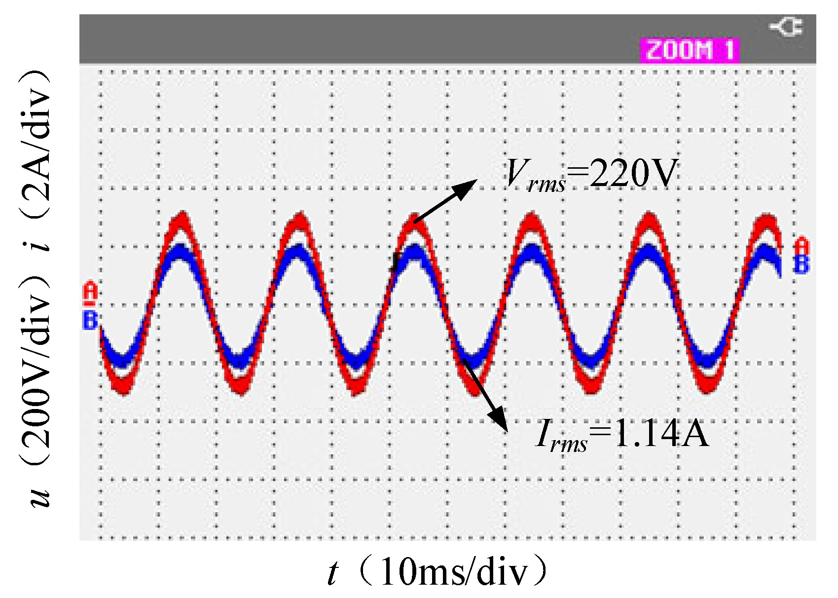
Figure 12 illustrates that the Phase-A voltage and current maintain RMS values of 220 V and 1.14 A, respectively, aligning with the 750 W active power setpoint. Furthermore, the voltage and current waveforms exhibit zero phase difference, verifying the 0 var reactive power output. Figure 13 confirms the successful grid connection of the inverter system, delivering 750 W of active power and 0 var of reactive power.

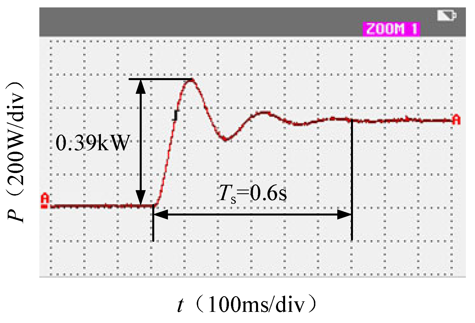
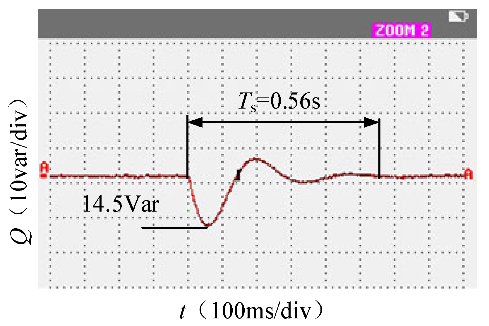
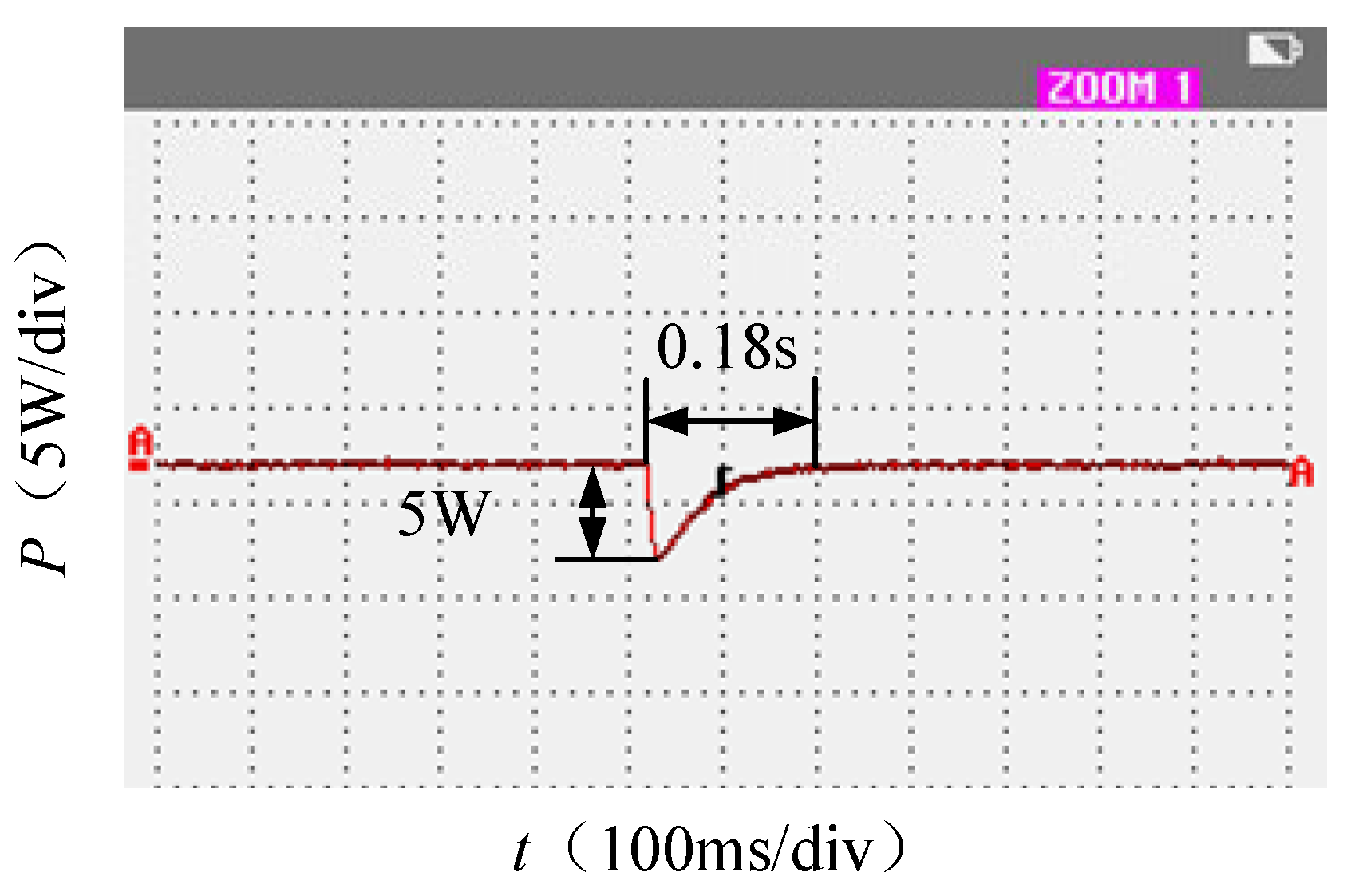
The transient trajectories for real (P) and imaginary (Q) power flows during an abrupt load increment are evaluated in Figure 13 and Figure 14, providing empirical evidence for the decoupling effectiveness of the recommended self-tuning impedance logic. A detailed inspection of the waveforms reveals that the control architecture successfully isolates the two regulation channels, effectively suppressing cross-loop interference throughout the dynamic transition. Regarding quantitative metrics, the real-power injection displays a 56% peak excursion and achieves stabilization within a 0.6 s window. Concurrently, the imaginary power baseline experiences a marginal deviation of 14.5 Var, recovering its equilibrium in 0.56 s. These outcomes verify that the current algorithm substantially fortifies the regulatory resilience of grid-interactive units in weak-inertia and sparsely damped environments, thereby ensuring enhanced network stability.

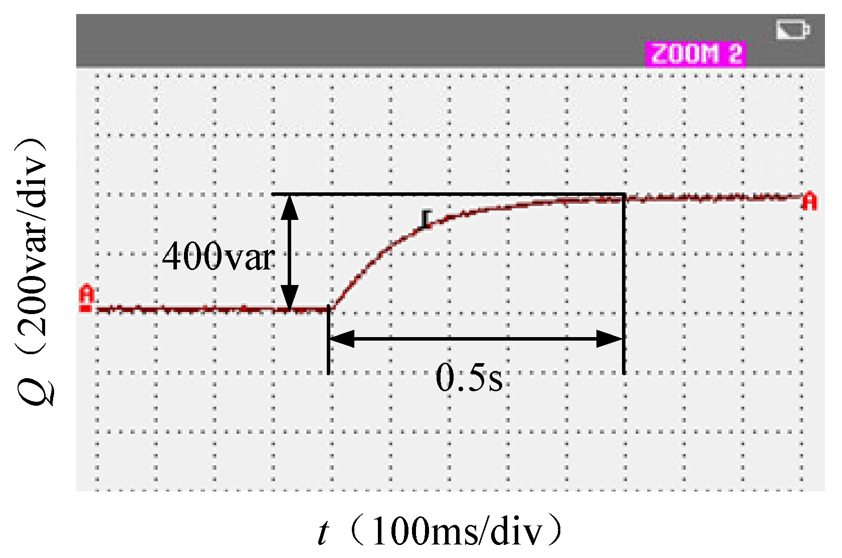
Control commands are issued via a supervisory workstation, maintaining a constant real-power target of 750 W throughout the test. Figure 15 and Figure 16 present the system’s dynamic trajectories when a reactive power step-change from 0 Var to 400 Var is triggered at the 5 s mark.

Empirical findings confirm that the recommended self-adaptive decoupling logic effectively isolates the active and reactive power channels during such transient events. Specifically, the real-power injection exhibits a minimal dynamic deviation of only 5 W with a rapid 0.4 s recovery period. Concurrently, the reactive power successfully tracks the new setpoint with a settling time of 0.52 s. A comprehensive review of the waveforms from Figure 12 through Figure 16 demonstrates that the implemented control paradigm successfully mitigates interactive cross-talk between the regulation loops. By leveraging this strategy, the inverter system achieves accelerated response times and fortified steady-state tracking precision, thereby validating its enhanced dynamic regulatory robustness and operational stability.

5. Conclusions

Driven by the imperative to stabilize renewable microgrids against the inherent volatility and low-inertia characteristics of integrated EV energy buffers, this research has established a rigorous analytical architecture for a novel two-stage cascaded C3PB bridge inverter. Recognizing that standard 3rd-order “quasi-steady-state” approximations fail to capture rapid electromagnetic transients—thereby misrepresenting system stability in weak-damping regimes—we derived a high-fidelity 5th-order electromagnetic-dynamic representation from the full-order state-space manifold. This refined model provides superior predictive accuracy and broadens the applicable parameter envelope for small-signal analysis.

Based on this advanced formulation, we introduced a self-adaptive dynamic virtual impedance decoupling technique that explicitly integrates both transient and steady-state factors. By dynamically neutralizing the interactive cross-talk between the active and reactive regulation channels, the strategy effectively rectifies the performance degradation triggered by strong loop coupling. Both numerical simulations and physical prototyping on a bespoke C3PB hardware platform corroborate the efficacy of the recommended strategy during grid disturbances. The experimental results confirm that, compared to legacy VSG methodologies, the proposed scheme achieves a significant leap in dynamic resilience, effectively isolating power flow interactions while enhancing the overall operational reliability of the inverter system.

References

1. Wen, T.; Zhu, D.; Zou, X.; Jiang, B.; Peng, L.; Kang, Y. Power Coupling Mechanism Analysis and Improved Decoupling Control for Virtual Synchronous Generator. IEEE Trans. Power Electron. 2020, 36, 3028–3041. [Google Scholar] [CrossRef] [Scilit]
2. Siwakoti, Y.P.; Palanisamy, A.; Mahajan, A.; Liese, S.; Long, T.; Blaabjerg, F. Analysis and Design of a Novel Six-Switch Five-Level Active Boost Neutral Point Clamped Inverter. IEEE Trans. Ind. Electron. 2019, 67, 10485–10496. [Google Scholar] [CrossRef] [Scilit]
3. Beck, H.-P.; Hesse, R. Virtual Synchronous Machine. In Proceedings of the International Conference on Electrical Power Quality and Utilization, Barcelona, Spain, 9–11 October 2007; pp. 1–6. [Google Scholar] [CrossRef] [Scilit]
4. Sun, J. Impedance-Based Stability Criterion for Grid-Connected Inverters. IEEE Trans. Power Electron. 2011, 26, 3075–3078. [Google Scholar] [CrossRef] [Scilit]
5. Wen, B.; Boroyevich, D.; Burgos, R.; Mattavelli, P.; Shen, Z. Analysis of D-Q Small-Signal1 Impedance of Grid-Tied Inverters. IEEE Trans. Power Electron. 2015, 31, 675–687. [Google Scholar] [CrossRef] [Scilit]
6. Coelho, E.A.; Cortizo, P.C.; Garcia, P.F.D. Small signal stability for single phase inverter connected to stiff AC system. In Proceedings of the IEEE Industry Applications Conference, Phoenix, AZ, USA, 3–7 October 1999; Volume 4, p. 2180. [Google Scholar]
7. Coelho, E.; Cortizo, P.; Garcia, P. Small-signal stability for parallel-connected inverters in stand-alone AC supply systems. IEEE Trans. Ind. Appl. 2002, 38, 533–542. [Google Scholar] [CrossRef] [Scilit]
8. Xiong, L.; Zhuo, F.; Wang, F.; Liu, X.; Chen, Y.; Zhu, M.; Yi, H. Static Synchronous Generator Model: A New Perspective to Investigate Dynamic Characteristics and Stability Issues of Grid-Tied PWM Inverter. IEEE Trans. Power Electron. 2015, 31, 6264–6280. [Google Scholar] [CrossRef] [Scilit]
9. Tan, S.; Geng, H.; Yang, G. Phillips-Heffron Model for Current-controlled Power Electronic generation Unit. J. Mod. Power Syst. Clean Energy 2017, 6, 582–594. [Google Scholar] [CrossRef] [Scilit]
10. Tan, S.; Geng, H.; Yang, G.; Wang, H.; Blaabjerg, F. Modeling framework of voltage-source converters based on equivalence with synchronous generator. J. Mod. Power Syst. Clean Energy 2018, 6, 1291–1305. [Google Scholar] [CrossRef] [Scilit]
11. Nikolakakos, I.P.; Zeineldin, H.H.; El-Moursi, M.S.; Hatziargyriou, N.D. Stability Evaluation of Interconnected Multi-Inverter Microgrids Through Critical Clusters. IEEE Trans. Power Syst. 2015, 31, 3060–3072. [Google Scholar] [CrossRef] [Scilit]
12. Mariani, V.; Vasca, F.; Vasquez, J.C.; Guerrero, J.M. Model Order Reductions for Stability Analysis of Islanded Microgrids with Droop Control. IEEE Trans. Ind. Electron. 2014, 62, 4344–4354. [Google Scholar] [CrossRef] [Scilit]
13. Vorobev, P.; Huang, P.-H.; Al Hosani, M.; Kirtley, J.L.; Turitsyn, K. High-Fidelity Model Order Reduction for Microgrids Stability Assessment. IEEE Trans. Power Syst. 2018, 33, 874. [Google Scholar] [CrossRef] [Scilit]
Figure 1. Schematic architecture of the recommended multi-level C3PB configuration using a two-stage cascaded layout.
Electronics 15 00241 g001
Figure 2. Operational mechanism and simplified equivalent diagram of the dual-stage C3PB unit.
Electronics 15 00241 g002
Figure 3. Comprehensive block diagram of the proposed control system.
Electronics 15 00241 g003
Figure 4. Physical interconnection and circuit layout for the grid-interactive inverter system.
Electronics 15 00241 g004
Figure 5. Equivalent circuit diagram representing the fifth-order dynamic model.
Electronics 15 00241 g005
Figure 6. State-space block diagram of the fifth-order electromagnetic dynamic system.
Electronics 15 00241 g006
Figure 7. Simplified network representation of the grid-connected VSG platform utilizing synthesized impedance parameters.
Electronics 15 00241 g007
Figure 8. Schematic overview of the adaptive virtual impedance decoupling control framework.
Electronics 15 00241 g008
Figure 9. Dynamic performance of the C3PB-based VSG under an abrupt increment in real power demand. (a) Transient trajectory of real power (P), (b) Evolution of imaginary power flow (Q).
Electronics 15 00241 g009
Figure 10. Inverter response characteristics following a stepwise increment in reactive demand. (a) Trajectory of Real Power Injection (P), (b) Transient Response of Imaginary Power (Q).
Electronics 15 00241 g010
Figure 11. Hardware configuration and laboratory testbed for the cascaded multi-level inverter system.
Electronics 15 00241 g011
Figure 12. Representative steady-state oscillograms of the Phase-A voltage and current generated by the prototype VSG.
Electronics 15 00241 g012
Figure 13. Dynamic trajectory of the real power injection during an induced stepwise active surge.
Electronics 15 00241 g013
Figure 14. Cross-coupling response of the imaginary power component following a P -channel disturbance.
Electronics 15 00241 g014
Figure 15. Transient cross-regulation of the real power channel during a stepwise reactive power transition.
Electronics 15 00241 g015
Figure 16. Dynamic response characteristics and tracking trajectory of the reactive power setpoint.
Electronics 15 00241 g016