An Improved Adaptive NSGA-II with Multiple Filtering for High-Dimensional Feature Selection

Abstract

As the number of feature dimensions increases, the decision-making space exhibits extensive and discrete characteristics, which poses a severe challenge to multi-objective (MO) evolutionary algorithms when searching for the optimal feature subset. Many existing algorithms face the difficulty of slow convergence speed and may fall into local optimal solutions. This study proposes AF-NSGA-II (an adaptive filtering-nondominated sorting genetic algorithm II), an improved MO evolutionary algorithm for high-dimensional feature selection, in which a novel sparse generation scheme for the solution set and an innovative adaptive crossover mechanism are introduced. This sparse initialization strategy, based on three distinct filter feature selection methods, produces initial solutions closer to the optimal Pareto solution set, which is beneficial for convergence. The adaptive crossover mechanism dynamically selects between geometric crossover operators (fostering convergence) and non-geometric crossover operators (enhancing diversity) based on parent similarity, effectively balancing both aspects and helping the algorithm to escape local optima. The algorithm is compared against six renowned multi-objective evolutionary algorithms across ten complex and publicly available datasets. The comparison results demonstrate the superiority of AF-NSGA-II over other algorithms, as well as its effectiveness in identifying the optimal feature subset.

1. Introduction

Classification represents a core learning task underlying numerous data analysis and decision-making applications [1]. In classification tasks, not all features contribute to the construction of a learning model. Indeed, some features may prove to be irrelevant or redundant, ultimately impairing the model’s classification performance. While the number of stored features can be extremely large in various datasets, a portion of them are redundant and need to be removed. The substantial presence of such features gives rise to the problem of storage costs and insufficient model learning, among other issues [2], and this problem becomes more prominent in the context of high-dimensional datasets. Prior to model training, appropriate data preprocessing is essential for mitigating these challenges. Improving learning efficiency has always been a central focus of research, with feature selection being a key priority. By discarding redundant and non-informative attributes, this process can substantially reduce computational cost while simultaneously enhancing predictive accuracy, generalization capability, and model interpretability [3].

Feature selection is employed to reduce computational complexity by limiting the number of features, while enhancing the model’s interpretability and contributing to improved classification accuracy [4]. Essentially, this process is categorized as an MO optimization task [5]. Assuming a dataset containing n features, there are $2^n-1$ total possible feature subsets. As n increases, the growth rate of $2^n-1$ accelerates, resulting in an enormous feature space that needs to be searched and making the identification of the optimal feature subset exceptionally challenging.

Recently, MO evolutionary algorithms have been favored by researchers for feature selection. Their effectiveness is often attributed to their excellent global search capabilities. These algorithms can expertly handle the complex task of selecting the most appropriate features from large datasets, underscoring their essential value in data analysis. Existing MOEA-based feature selection methods primarily include the MO differential evolution algorithm, which learns the differential mutation between biological populations [6]; the MO particle swarm algorithm, which learns foraging behavior to enhance the optimization process [7]; the MO grey wolf optimization algorithm, which learns hunting behaviors such as “surrounding, chasing, and attacking” from grey wolves [8]; the MO ant colony algorithm, which updates through pheromone [9]; the MO artificial bee colony algorithm, which achieves a balance among multiple optimization objectives through Pareto dominance and archive maintenance [10]; and the MO genetic algorithm, which learns genetic mutations [11]. Among these, binary-coded MO genetic algorithms, which conveniently represent feature selection processes, are the most widely used [12]. However, as feature dimensionality increases, MO genetic algorithms still exhibit significant limitations when confronted with the mismatch between high-dimensional feature spaces and their algorithmic characteristics: (1) Owing to the insufficient search capability of common genetic operators, these algorithms fail to balance convergence and diversity [13], thereby preventing the algorithm from achieving optimal search performance and resulting in relatively poor experimental results. (2) The neglect of implicit information in datasets during random population initialization causes the initial population to be far from the optimal Pareto solution set, which is a particularly significant disadvantage in high-dimensional feature selection that hinders algorithm convergence.

To mitigate the aforementioned issues, this study proposes AF-NSGA-II, an improved MO evolutionary algorithm for high-dimensional feature selection. The main contributions of this study are summarized as follows:

(1)

A population sparse initialization method, in conjunction with multiple filter techniques, is proposed to guide the initial solutions toward the optimal Pareto front, thereby accelerating algorithm convergence and reducing the iteration count.

(2)

An adaptive crossover mechanism is designed based on the similarities of parent individuals to ensure both the spread of solutions and the approach towards the optimal solution during the evolution process.

2. Related Work

2.1. MO Optimization Definition

MO optimization involves simultaneously addressing multiple conflicting objectives [14,15]. As an example, consider the minimization of multiple objectives, which can be formally expressed as:

$$\begin{array}{cc}\hfill & \mathrm{Minimize}\mathcal{F}\left(y\right)=[f_1\left(y\right),f_2\left(y\right),\dots ,f_m\left(y\right)]\hfill \\ \hfill & \mathrm{subject}\mathrm{to}\left\{\begin{array}{c}{p}_k\left(y\right)\ge 0,k=1,2,\dots ,n\hfill \\ q_l\left(y\right)=0,l=1,2,\dots ,o\hfill \\ A_k\le y_k\le B_k,k=1,2,\dots ,p\hfill \end{array}\right.\hfill \end{array}$$

(1)

$$y=[y_1,y_2,\dots ,y_d]$$

denotes a collection of decision variables, where d specifies the dimensionality of the variable set and m indicates the total number of objectives to be optimized simultaneously. $p_k\left(y\right)$ corresponds to the k-th inequality constraint, and $q_l\left(y\right)$ corresponds to the l-th equality constraint. A candidate solution y is regarded as feasible only if all these constraints are fulfilled. Additionally, $[A_k,B_k]$ defines the permissible interval for the variable $y_k$.

2.2. Filtering Methods

2.2.1. ReliefF

The ReliefF [16] algorithm is a well-established feature selection method that relies on distance-based criteria and is capable of addressing multi-class classification problems. The weighted distance between instances effectively distinguishes the categories of the instances. A smaller distance indicates that the two categories are more similar, whereas a larger distance indicates that the two categories are more distinct.

$$W\left(f_i\right)=-\sum _{j=1}^K{\displaystyle \frac{\Delta (f_i,R_s,H_j)}{M·K}}+\sum _{C\ne \mathrm{class}\left(R_s\right)}\left[{\displaystyle \frac{P\left(C\right)}{1-P\left(\mathrm{class}\left(R_s\right)\right)}}\sum _{j=1}^K{\displaystyle \frac{\Delta (f_i,R_s,M_j)}{M·K}}\right]$$

(2)

$$\Delta (f_i,X,Y)=\left\{\begin{array}{cc}0\hfill & \mathrm{if}{f}_i\mathrm{is}\mathrm{categorical}\mathrm{and}X\left[f_i\right]=Y\left[f_i\right]\hfill \\ 1\hfill & \mathrm{if}{f}_i\mathrm{is}\mathrm{categorical}\mathrm{and}X\left[f_i\right]\ne Y\left[f_i\right]\hfill \\ {\displaystyle \frac{X\left[f_i\right]-Y\left[f_i\right]}{max\left(f_i\right)-min\left(f_i\right)}}\hfill & \mathrm{if}{f}_i\mathrm{is}\mathrm{numerical}\hfill \end{array}\right.$$

(3)

Suppose the dataset contains L classes, denoted as $C=c_1,c_2,\dots ,c_L$. For a sample $R_s$ belonging to class $c_l$, the ReliefF algorithm begins by randomly selecting $R_s$ and locating K closest points from the same class, denoted as $H_j$ ($j=1,2,\dots ,K$). Subsequently, K nearest points are identified in each of the remaining classes, labeled as $M_j$ ($j=1,2,\dots ,K$). This procedure is performed for every feature $f_i$, and the corresponding feature score is calculated using Equation (2). Here, M refers to the total number of repetitions, and $P\left(C\right)$ indicates the likelihood of class C. The operator $\Delta (f_i,X,Y)$, which measures the discrepancy between instances X and Y with respect to feature $f_i$, is specified in Equation (3).

2.2.2. Variable Association

The Maximum Information Coefficient (MIC) [17] is employed to evaluate complex variable interactions and assess their nonlinear relationships. MIC measures both linear and nonlinear relationships between variables within large datasets, as well as uncovering non-functional dependencies. The core concept is that if a correlation exists between two variables, the distribution of data points in a grid, after partitioning the scatter plot, can reveal their relationship.

The MIC primarily relies on mutual information and grid partitioning for its computation. Let U and V represent a pair of random variables with a sample size of n. When the scatter plot of U and V is divided into an R-by-S grid, the mutual information between U and V can be calculated as follows:

$$I(U,V)=\sum _{u_i\in U,v_j\in V}p(u_i,v_j)log{\displaystyle \frac{p(u_i,v_j)}{p\left(u_i\right)p\left(v_j\right)}}$$

(4)

Here, $p(u_i,v_j)$ denotes the joint probability density function (PDF) of U and V, while $p\left(u_i\right)$ and $p\left(v_j\right)$ denote the marginal PDFs of U and V, respectively. The estimation of these joint and marginal probabilities is conducted via grid partitioning. Moreover, the grid dimensions R and S must satisfy the condition $RS<L$, where $L=n^{0.6}$.

The MIC between U and V is then computed as:

$$MIC(U;V)=\underset{RS<L}{max}{\displaystyle \frac{I^{*}(U,V)}{log\left(min(R,S)\right)}}$$

(5)

where $I^{*}(U,V)$ represents the maximum mutual information for given grid dimensions R and S, obtained by adjusting the grid boundaries. For comparability across different feature scales, this maximum mutual information is normalized to lie within the interval [0, 1]. An MIC value of 0 indicates complete independence between the variables, whereas values approaching 1 suggest a stronger association. In this study, the MIC metric is used to quantify the dependence between features and the target label, with higher MIC values indicating a stronger relationship.

2.2.3. Fisher Score

The Fisher Score [18] identifies the features that maximize the within-class variance and minimize the between-class variance, thereby assessing the importance of the features. Its objective is to identify features that not only maximize between-class scatter, but also minimize within-class scatter. The Fisher Score calculates a score to each feature in the dataset and selects a certain number of high-scoring features to form a feature subset. The Fisher calculation formula for feature $F_i$ is as follows:

$$Fisher\left(F_i\right)={\displaystyle \frac{{\displaystyle \sum _{k=1}^c}{n}_k{({\mu }_k^i-{\mu }^i)}^2}{{\displaystyle \sum _{k=1}^c}{n}_k{\left({\sigma }_k^i\right)}^2}}$$

(6)

Here, for the k-th class of samples, $n_k$ represents the total number of samples in that class, with ${\mu }_k^i$ and ${\sigma }_k^i$ denoting the mean and standard deviation of the i-th feature, respectively. Additionally, ${\mu }^i$ represents the mean of the i-th feature across all classes. The Fisher Score assesses the discriminatory power of features, with a higher value of $Fisher\left(Fi\right)$ indicating stronger discriminatory ability for the corresponding feature.

2.3. Geometric Crossover and Non-Geometric Crossover

In Evolutionary Multi-Objective Optimization (EMO) algorithms, traditional mask-based crossover operators (such as priority-based mask crossover, shuffle crossover, and uniform crossover [19,20]) primarily accelerate the convergence process within specific regions of the Pareto front [21]. These operators also restrict the diversity of solutions along the front. This effect arises from the operational constraints of these methods, categorized as geometric crossovers [22]. Specifically, offspring produced by these operators are always located within the linear segment connecting their two parents in the Hamming space of genotypes. Consequently, the combined distances from the offspring to each parent exactly equal the Hamming distance separating the parents.

The following presents the definition of the geometric crossover operator. Suppose there exists an offspring individual, denoted as w, generated by a specific crossover operator, which is an operation in genetic algorithms that simulates gene exchange between two parent individuals, denoted as a and b. If a crossover operator’s decision variables are continuous real numbers, the offspring are non-discrete, and the offspring are generated by combining the geometric space of the parents, then it is a geometric crossover operator. In this case, a specific relationship holds among a, b, and w:

$$\rho (a,w)+\rho (b,w)=\rho (a,b)$$

(7)

Conversely, if there does not exist any distance function that satisfies the specified relationship (7), then the operator is classified as a non-geometric crossover operator [21]. Such operators possess certain characteristics. These operators can enhance solution dispersion along the Pareto front within EMO algorithms. Importantly, although they increase the spread of solutions, they do not substantially deteriorate the convergence properties of these algorithms [21]. This characteristic makes them valuable in scenarios requiring broader exploration of the solution space without significantly compromising convergence.

The classical non-geometric crossover operator [21] is defined as follows. For the parent individuals x and y, the superior parent—i.e., the non-dominant individual—is initially selected as the primary parent (assumed to be x), while the other parent serves as the secondary parent. The process of generating the offspring, denoted as z, from the parent individuals x and y is carried out in a specific manner. Initially, all the genes of the primary parent x are replicated precisely to the offspring z. Subsequently, in cases where the genes are identical between x and the secondary parent y, the offspring z undergoes a bitwise flip of these genes with a probability denoted by $P_{BF}$. This method is depicted in Figure 1. From the perspective of the offspring individual generation process, the geometric crossover operator has a unique mechanism of action. It becomes apparent that the geometric approach ensures that each gene position in the offspring must correspond to the gene of at least one parent; that is, either x or y. On the contrary, utilizing a non-geometric crossover operator allows for the possibility that a gene at any position in the offspring z may not match the genes from either parent. Suppose that we represent the genes at the $ith$ position of the parent individuals x, y and the offspring individual z as a triple $gene=(x_i,y_i,z_i)$. Generally speaking, the genes here are binary-coded, where 0 and 1 represent different states or characteristics. When the geometric crossover operator is applied to generate offspring z, there are six possible gene-combination scenarios. Specifically, these combinations are (0, 0, 0), (0, 1, 0), (0, 1, 1), (1, 0, 0), (1, 0, 1), and (1, 1, 1). However, combinations such as (0, 0, 1) and (1, 1, 0) do not occur during the process of generating offspring using the geometric crossover operator. Nevertheless, when a non-geometric crossover operator is employed to generate the offspring z, the situation is quite different. It does not have the strict gene-combination constraints, and all eight gene combinations mentioned above—namely, (0, 0, 0), (0, 0, 1), (0, 1, 0), (0, 1, 1), (1, 0, 0), (1, 0, 1), (1, 1, 0), and (1, 1, 1)—may occur.

2.4. Literature Review

NSGA-II is a classic algorithm in the context of MOEAs, and has been widely applied due to its suitability for problems with either continuous or discrete decision variables [23]. Within the domain of feature selection, Hamdan et al. [24] were pioneers in introducing multi-objective feature selection to low-dimensional datasets using NSGA-II. Their results demonstrated that the solution quality continuously improved throughout the evolutionary process until convergence. Wang et al. [25] proposed a feature selection algorithm based on grid domination and subset filtering mechanisms to significantly enhance the diversity of the population. Rehman et al. [26] proposed a subset selection method from the perspective of decision fairness and legitimacy in supervised machine learning models. Their goal was to balance fairness and accuracy by removing features that were most likely to bias decision-making. The results demonstrated that NSGA-II plays a significant role in ensuring fairness in machine learning models. Xue and colleagues [11] introduced an interval-based initialization strategy and an adaptive crossover mechanism within the NSGA-II framework, aimed at precisely determining the number of features to be selected for offspring. However, although this approach is innovative in certain aspects, it does not consider feature–label correlations and the exploration efficiency of its operators is constrained by feature weights. Although the refinements in initialization and crossover operations enhance the algorithm’s adaptability in feature selection, these adjustments lack a multidimensional assessment of feature importance and could lead to inadequate search capabilities due to the limitations imposed by feature weights. Gong et al. [27] achieved the avoidance of ineffective search results by designing variable-length individual encoding to replace traditional fixed-length encoding, and introduced a local search to enhance the robustness of the algorithm. Li et al. [28] conducted innovative research: building on the NSGA-II algorithm framework, they introduced a greedy repair strategy and enhanced the population initialization, selection, and mutation operators. Subsequently, they proposed a novel hybrid feature selection algorithm to address the challenges associated with high-dimensional, multi-objective feature selection. This algorithm integrates various enhancement mechanisms, aiming to precisely select feature subsets from high-dimensional data and boost the efficiency and effectiveness of subsequent data analysis and modeling. However, the algorithm exhibits several limitations. The filter-based method it employs is considered overly simplistic, which limits the algorithm’s search capability, thereby reducing the accuracy of the evaluation results. Moreover, the algorithm’s stability is poor, exhibiting significant fluctuations under various conditions. There is considerable room for improvement in both the accuracy and stability of the algorithm. Jiao et al. [29] transformed the feature selection problem into a bi-objective problem through sparse learning and automatic loss balancing, and proposed an initialization strategy adapted to the bi-objective problem. However, this method neglects the correlation between the mask part of the solution and the coefficient matrix, leading to a decline in feature selection performance. Vijai et al. [30] improved its efficiency by leveraging the advantages of filter-based methods, incorporating techniques such as random forests. They also designed a crossover mutation operator to clarify the search direction.

3. Proposed Method

3.1. Framework of AF-NSGA-II

The framework of the AF-NSGA-II algorithm is presented in Algorithm 1. Initially, the ReliefF, MIC, and Fisher score methods are employed to assess the relevance of features and labels within the dataset ($DS$), and corresponding weights are assigned to the features based on their relevance to the labels. Subsequently, the entropy weight method is employed to assign weights to the ReliefF, MIC, and Fisher score methods, resulting in the final feature weights, which are recorded in the vector $FW$. Following this, the population sparsity initialization is guided by $FW$ to form a population P consisting of N individuals. Next, to ensure the preservation of high-quality genetic features in subsequent generations, 2N individuals are selected from the population P based on each individual’s non-dominant front number and crowding distance. The parent population $P_p$ is then constructed through binary tournament selection. In the next step, N pairs of parents undergo adaptive crossover based on parental similarity, and a mutation operator referencing feature weight information is applied to generate N offspring, forming the offspring population $P_o$. Next, $P_o$ and P are merged to form the population R. Duplicate individuals in R are eliminated in the decision space, and an environmental selection operation is conducted to retain N superior individuals, forming the new population. The evolution continues until the maximum number of individual evaluations is reached.

Algorithm 1 Framework of AF-NSGA-II.

Require: D (number of features), N (population size), $DS$ (dataset) Ensure: Optimal feature subset   1: Get the feature weights $FW$;                                                      ▹ Algorithm 2   2: Initialize population P based on $FW$;                                       ▹ Algorithm 3   3: while termination criterion not fulfilled do   4:       $P_p\leftarrow$ Select $2N$ parents via binary tournament selection   5:       $P_o\leftarrow$ adaptiveCrossover($P_p$)                                                ▹ Algorithm 4   6:       $P_o\leftarrow$ Mutation($P_o$, $FW$)                                                         ▹ Algorithm 5   7:       $R\leftarrow P_o\cup P$   8:       Delete duplicated solutions from R in decision space   9:       $P\leftarrow$ environmentalSelection(R) 10: end while 11: Select non-dominated solutions in P as $PF$ 12: Optimal feature subset $\leftarrow PF$ return Optimal feature subset

Algorithm 2 Get Feature Weights ($DS$).

Require: $DS$ (dataset) Ensure: $FW$ (feature weights)   1: $D\leftarrow$ Number of features in $DS$   2: $FW\leftarrow$$1\times D$ matrix of zeros   3: $reff\leftarrow$ ReliefF($DS$)   4: $mic\leftarrow$ MIC($DS$)   5: $fisher\leftarrow$ FisherScore($DS$)   6: PositiveNormalize($reff$, $mic$, $fisher$)   7: $[w_{reff},w_{mic},w_{fisher}]\leftarrow$ EntropyWeightMethod($reff$, $mic$, $fisher$)   8: for$i=1$to D do   9:       $F{W}_i\leftarrow w_{reff}\times ref{f}_i+w_{mic}\times mi{c}_i+w_{fisher}\times fishe{r}_i$ 10: end for         return $FW$

Algorithm 3 Initialization(D, N, $FW$).

Require: D (number of features), N (population size), $FW$ (feature weights) Ensure: P (initial population) 1: $P\leftarrow$$N\times D$ matrix of zeros 2: for $p\in P$ do 3:       $n\_sf\leftarrow rand\times D$                                                   ▹$n\_sf$ is between 0 and D 4:       $sf\_idx\leftarrow$ tournamentSelection($n\_sf$, $FW$) 5:       $p(sf\_idx)\leftarrow 1$ 6: end for         return P

Algorithm 4 AdaptiveCrossover(P).

Require: P (a set of parents) Ensure: O (a set of offsprings)   1: $O\leftarrow \varnothing$   2: Initialize $OPHD$ according to (11)   3: $AM\leftarrow 2\times m$ matrix of zeros   4: $SM\leftarrow 2\times m$ matrix of zeros   5: $M_{hd}\leftarrow \lfloor {log}_{2}N+1\rfloor$   6: $all\_hd\leftarrow [2,3,\dots ,M_{hd}-1,M_{hd}]$   7: for$i=1\mathbf{to}N$do   8:       $[P1,P2]\leftarrow$ Select two parents from P in order   9:       $hd\leftarrow HD(P1,P2)$ 10:       if $hd\le 1$ then 11:            $o\leftarrow$ NonGeometric_Crossover($P1,P2$) 12:       else if $hd>M_{hd}$ then 13:            $o\leftarrow$ Uniform_Crossover($P1,P2$) 14:       else 15:            $hd\_idx\leftarrow$ Find index of $hd$ in $all\_hd$ 16:            $hd\_idx\leftarrow hd\_idx+1$ 17:            $p\_uni\leftarrow OPH{D}_{1,hd\_idx}$ 18:            $p\_ngeo\leftarrow OPH{D}_{2,hd\_idx}$ 19:            $operator\_idx\leftarrow$ Roulette($p\_uni,p\_ngeo$) 20:            if $operator\_idx=1$ then 21:                 $o\leftarrow$ Uniform_Crossover($P1,P2$) 22:            else 23:                 $o\leftarrow$ NonGeometric_Crossover($P1,P2$) 24:            end if 25:            $A{M}_{operator\_idx,hd\_idx}\leftarrow A{M}_{operator\_idx,hd\_idx}+1$ 26:            if $P1\mathrm{not}\mathrm{dominated}\mathrm{by}o\mathrm{and}P2\mathrm{not}\mathrm{dominated}\mathrm{by}o$ then 27:                 $S{M}_{operator\_idx,hd\_idx}\leftarrow S{M}_{operator\_idx,hd\_idx}+1$ 28:            end if 29:        end if 30:        $O\leftarrow O\cup o$ 31: end for         return O

Algorithm 5 Mutation(O, $FW$).

Require: O (a set of offsprings), $FW$ (weights of features) Ensure: O (a set of offsprings)   1: for$o\in O$do   2:     if $rand<0.5$ then   3:           $nz\_idx\leftarrow$ find all indices of nonzero elements in o   4:           $m\_idx\leftarrow$ tournamentSelection($nz\_idx,FW$)   5:           $o(m\_idx)\leftarrow 0$   6:     else   7:           $z\_idx\leftarrow$ find all indices of zero elements in o   8:           $m\_idx\leftarrow$ tournamentSelection($z\_idx,FW$)   9:           $o(m\_idx)\leftarrow 1$                                                  ▹ mutation: set zero element to one 10:     end if 11: end for         return O

3.2. Computational Complexity Analysis

The primary computational demand of AF-NSGA-II originates from the hierarchical sorting procedure and crowding distance evaluation. Specifically, the sorting process requires $O\left(M{N}^2\right)$ operations, where N denotes the population size and M represents the total number of objectives. In addition, binary-encoded crossover and mutation introduce $O\left(ND\right)$ operations, with D corresponding to the dimensionality of the features. Hence, for each generation, both NSGA-II and AF-NSGA-II entail a per-generation cost of $O(M{N}^2+ND)$.

AF-NSGA-II also incorporates several auxiliary components, which impose relatively minor computational demands. Assessing feature relevance through ReliefF, MIC, and Fisher Score involves $O\left(S{D}^2\right)$ operations, where S stands for the sample count. This evaluation is conducted solely during the initialization phase, making it independent of the number of generations. The similarity-driven crossover procedure, which uses Hamming distance measurements and probabilistic selection, requires $O\left(ND\right)$ operations, comparable to conventional crossover routines. Likewise, the mutation operator guided by feature weights incurs $O\left(ND\right)$ linear operations and does not notably increase the computational effort.

Consequently, the total computational requirement of AF-NSGA-II can be expressed as:

$$O\left(T(M{N}^2+ND)+S{D}^2\right),$$

(8)

where T indicates the maximum number of generations. Since the $S{D}^2$ term appears only during initialization, the asymptotic computational behavior of AF-NSGA-II aligns with that of the standard NSGA-II. Memory usage is dominated by population storage, yielding $O\left(ND\right)$ in space complexity.

3.3. Objective Functions

Given the common occurrence of unbalanced data within numerous high-dimensional datasets, this study utilizes both the balanced error rate (BER) [31] and the fraction of selected features to evaluate individuals as part of its fitness function. The BER is specified as follows:

$$balanced\_err=1-{\displaystyle \frac{1}{c}}\sum _{i=1}^{c}TP{R}_i$$

(9)

where c represents the number of classes in the problem, and $TP{R}_i$ denotes the true positive ratio, which is the proportion of correctly identified instances in class i. Since no class is favored over another, the weight for each class is assigned a value of $1/c$. The definition of the selected feature ratio is provided below:

$$\mathrm{feature}\mathrm{selection}\mathrm{ratio}={\displaystyle \frac{d}{D}}$$

(10)

where d denotes the number of selected features, and D refers to the total number of features.

3.4. Sparse Initialization Referring to Feature Weights

In this paper, a binary encoding scheme represents individuals (chromosomes) in the population. The length of each chromosome corresponds to the dimensionality of the feature. On these chromosomes, gene values are binary, with 1 indicating feature inclusion and 0 indicating feature exclusion.

In the context of high-dimensional data, the feature selection problem constitutes a sparse optimization problem, characterized by most decision variables in the optimal solution being zero. However, many existing MO evolutionary algorithms fail to account for the sparsity characteristic of the optimal solution when addressing high-dimensional feature selection challenges. They commonly randomly initialize the population, assigning each feature a 50% chance of inclusion in the feature subset. This leads to most initial solutions displaying similar quantities of 0 and 1 values among their decision variables, resulting in the majority being significantly distant from the optimal Pareto front—a scenario which detrimentally affects the algorithm’s early convergence. Considering this, Xue et al. [1] and Li et al. [28] introduced and refined the sparse initialization strategy of the large-scale sparse MO evolutionary algorithm SparseEA [32], for handling feature selection problems. By integrating the distance-based filter feature selection method, ReliefF, for sparse initialization, they effectively accelerated the algorithm’s early convergence. However, as only the distance metric criterion was utilized to evaluate the features, the accuracy and stability of the feature evaluation results were not assured.

To address the limitations and shortcomings of adopting a single feature metric criterion, three filtering methods with different evaluation criteria are employed. Additionally, the entropy weight method is applied to objectively assign weights to these methods.This approach not only utilizes the advantages of the methods with different evaluation criteria, but also aims to obtain more stable and accurate feature evaluation results. This can guide the population sparse initialization and accelerate the convergence of the algorithm.

The specific process of population initialization can be described as follows. Initially, correlations between all features and labels are evaluated using the ReliefF, MIC, and Fisher score methods, with weights subsequently assigned to each feature based on these correlations. The greater the correlation between a feature and a label, the more significant its contribution to correct classification, resulting in a higher weight being assigned to that feature. After obtaining the feature weight information $reff$, $mic$, $fisher$ using the ReliefF, MIC, and Fisher score methods, this data is normalized and then integrated using the entropy weighting method to assign weights objectively across the three filter methods. This process yields the final feature weight information, which is recorded in the feature weight vector $FW$ and used to guide the population initialization.

This random integer is denoted as $n\_sf$, which is greater than 1 and less than the feature dimension D. The features for each individual, $n\_sf$ in number, are selected through a binary tournament based on $FW$. For example, consider a dataset $DS$ with a feature dimension $D=6$ and a feature weight vector $FW=(0.07,0.15,0.13,0.3,0.25,0.1)$. During the initialization of individual X, a random integer $n\_sf=2$ is generated. Following the binary tournament based on $FW$, the resulting encoding of individual X is likely 000110, indicating that the fourth and fifth features—which have higher weights—are likely selected. The initialization procedure of the population is detailed in Algorithms 2 and 3. It is worth noting that feature sparsification is explicitly achieved by randomly controlling $n\_sf$, the count of active features assigned to every member of the population, where $n\_sf\ll D$, and choosing a limited portion of features according to the feature weight vector $FW$. Consequently, the majority of decision variables are initialized to zero, producing a sparse population in the decision space.

3.5. Adaptive Crossover Based on Parental Similarities

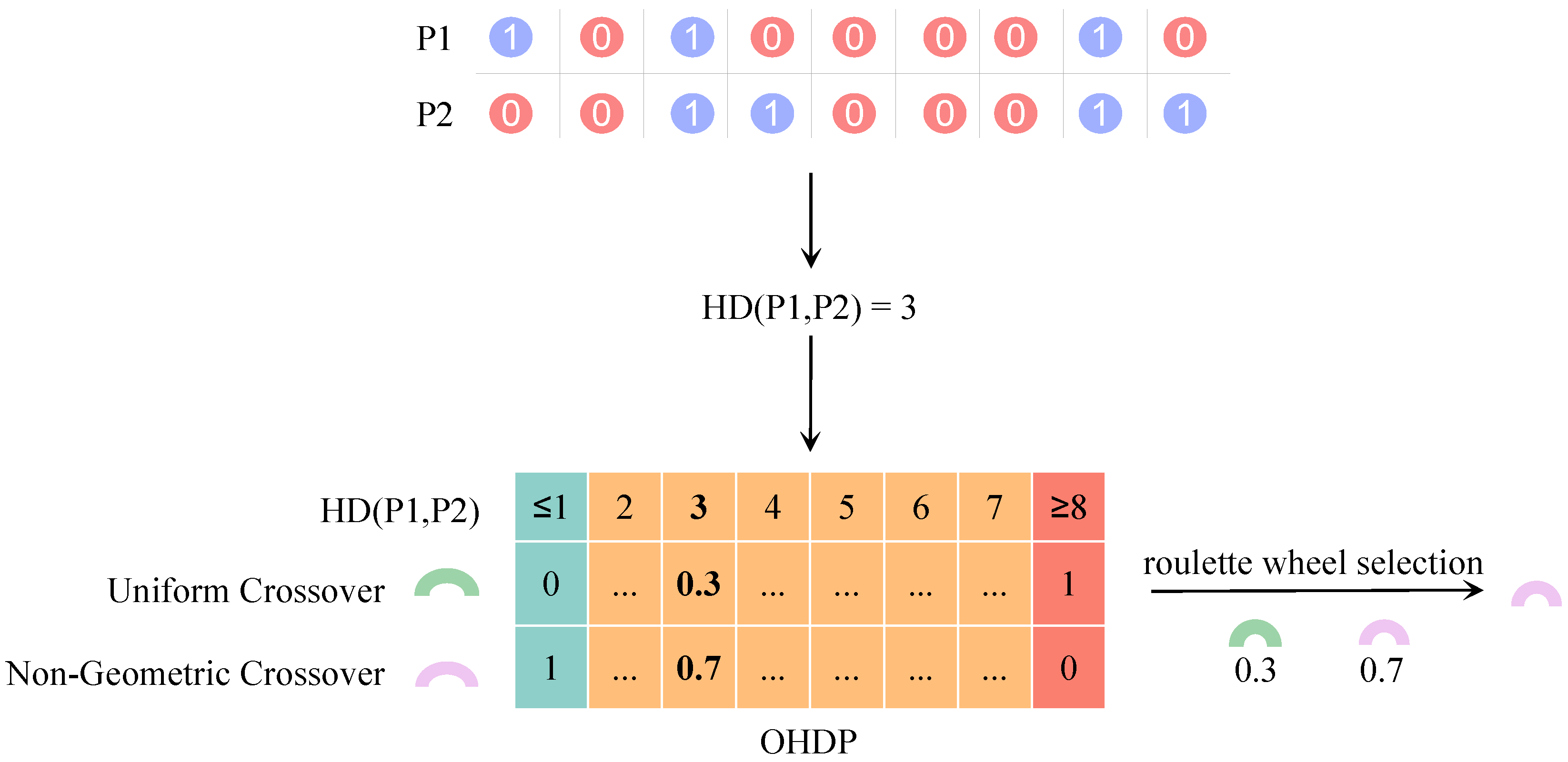
For example, if two parent feature subsets have a Hamming distance of $hd=3$, they are regarded as moderately similar. According to the OHDP matrix, the non-geometric crossover is selected with a higher probability (0.7) via roulette wheel selection to generate the offspring.

In addition, a brief statistical observation was conducted during the evolutionary process. We found that, for parent pairs with moderate similarity ($hd\in [2,\lfloor {\log }_{2}N\rfloor +1]$), the offspring generated by the non-geometric crossover exhibited a higher probability of being non-dominated compared with those produced by the geometric crossover, which supports the effectiveness of the proposed adaptive selection strategy.

In MO evolutionary algorithms, crossover is the primary mechanism in searching for new solutions. The crossover results depend on the crossover operator and the crossover probability; research indicates that various crossover operators are suitable for different optimization problems, and distinct crossover probabilities are suitable for different evolutionary stages. Therefore, implementing an adaptive crossover could significantly enhance the search capability of evolutionary algorithms. Existing studies on adaptive crossover primarily focus on the dynamic selection of different geometric crossover operators [33] and crossover probabilities [34], often overlooking how well solutions converge while maintaining diversity across the population. From the perspective of balancing convergence and diversity, the adaptive selection of crossover operators with varying search characteristics can enhance the search capability of evolutionary algorithms. Consequently, we combine the search characteristics of different crossover operators and propose an adaptive crossover mechanism based on parent similarity. This mechanism has been incorporated into NSGA-II to mitigate issues caused by high feature dimensionality, reduce computational cost, and enhance generalization capability. It is worth noting that the proposed adaptive crossover mechanism is applicable across all evolutionary algorithms that use binary coding and incorporate crossover operators.

The adaptive crossover mechanism presented in this study dynamically employs various crossover operators to generate offspring based on parental similarity, thus effectively balancing both convergence and diversity. When parents exhibit high genetic similarity, a non-geometric crossover operator—designed specifically to enhance diversity—is employed. Conversely, for parents with low genetic similarity, a geometric crossover operator—which facilitates convergence—is utilized. For parents exhibiting moderate genetic similarity, the selection of the crossover operator (either geometric or non-geometric) depends on its past performance in generating viable offspring. The similarity between two parental genotypes, X and Y, is determined by their Hamming distance, as shown in (10). A greater Hamming distance indicates a lesser genetic overlap and, consequently, reduced similarity.

$$HD(X,Y)=\sum _{i=1}^N{X}_i\oplus Y_i$$

(11)

To achieve adaptive crossover based on parent similarity according to the search characteristics of different crossover operators, this section explores the relationship between parent similarity and both geometric and non-geometric crossover operators. When the Hamming distance $hd$ between a pair of parents is 0 or 1, indicating that the parents are either completely identical or differ by only one gene, they are considered to have a high level of similarity. If this pair of parents employs a geometric crossover operator to generate offspring (where two parents produce one offspring as discussed), the resulting offspring generated will not dominate the parents and will likely be identical to one of them. This not only wastes evaluation opportunities, but also does not contribute to improving the diversity of solutions within the population. Therefore, when a pair of parents exhibits a high similarity level, only non-geometric crossover operators should be employed to generate offspring, potentially producing better offspring and enhancing the diversity of the population.

When the Hamming distance between a pair of parents is 2, the two parents differ in exactly two genes. In this case, using a geometric crossover operator to generate offspring results in a 50% chance that the offspring will be identical to one of the parents. When the Hamming distance is 3, the geometric crossover operator yields a 25% chance that the offspring will be identical to one of the parents. Accordingly, when $hd$ represents the Hamming distance between two parent chromosomes, the probability that the offspring produced by a geometric crossover approach will replicate one of the parent genotypes is $1/2^{hd-1}$. Considering an extreme scenario where the Hamming distances $hd$ of N pairs exceed ${log}_{2}N+1$, and these pairs solely employ the geometric crossover for reproduction. The expected number of offspring identical to a parent among the N is less than one. This implies that, in practice, it is almost impossible for any of these N offspring to be identical to either parent. Therefore, when the Hamming distance between a pair of parents exceeds ${log}_{2}N+1$, it is considered to indicate a low similarity level between parents. When a pair of parents display low similarity, the employment of the geometric crossover technique for producing offspring is advisable. This approach ensures that the resulting offspring infrequently resemble either parent, thereby maintaining diversity among solutions while leveraging the operator’s capacity to facilitate convergence.

When the Hamming distance $hd$ between a pair of parents is within the range $\left[2,{log}_{2}N+1\right]$, the pair is considered to exhibit moderate similarity. When parents exhibit moderate similarity, using a geometric crossover operator can result in offspring identical to either parent with a certain probability. Simultaneously, there is a probability that offspring generated may dominate the parents or be dominated by them. This principle applies equally with a non-geometric crossover operator. As the evolutionary phase advances, and the Hamming distance $hd$ between parents ranges from 2 to $\lfloor {log}_{2}N+1\rfloor$, the effectiveness of both geometric and non-geometric crossover operators changes, the probability that offspring generated by the geometric crossover operator will differ from their parents. Therefore, when a pair of parents exhibits moderate similarity, the selection of the crossover operator should be adaptive, based on historical performance data across various Hamming distances, to optimize each operator’s benefits and enhance the evolutionary algorithm’s search efficacy. This study introduces a probability-based adaptive selection mechanism for crossover operators. Specifically, there are m ($m=⌊{log}_{2}N⌋$+2) distinct values of the Hamming distance between the parents and, to achieve adaptive selection of crossover operators under varying Hamming distances at different evolutionary stages, the $OPHD$ matrix records the probability of selecting each crossover operator ($OPH{D}_{n,m}$ denotes the probability of selecting the nth operator at the mth Hamming distance). Whenever a pair of parents at a moderate similarity level undergoes crossover to generate offspring, these selection probabilities are retrieved from the $OPHD$ matrix based on the Hamming distance. The initial state of the $OPHD$ matrix is zero-filled, except for its first and last columns, and it is updated each generation. The probability that each crossover operator will produce superior offspring, as observed in the previous generation, determines its selection probability for the next generation’s parental crossover. Superior offspring are defined as those that are not dominated by any parent.

To calculate the probability of each crossover operator producing superior offspring, and to update the $OPHD$ according to (11), the two matrices $AM$ and $SM$ record the selection counts and the counts of superior offspring produced by each crossover operator at various Hamming distances, respectively. This approach enables adaptive selection of crossover operators at different Hamming distances during various evolutionary stages. Furthermore, since there is only one empirically validated non-geometric crossover operator [21] used in this study, to ensure fairness, only the uniform crossover operator was selected as the geometric crossover operator.

$$OPH{D}_{n,m}={\displaystyle \frac{S{M}_{n,m}}{A{M}_{n,m}}},\mathrm{s}.\mathrm{t}.1<m<\lfloor {log}_{2}N\rfloor +2$$

(12)

An example of adaptive crossover based on parental similarity is illustrated in Figure 2, assuming that the population size $N=100$ and $HD(P1,P2)$ = 3. Since $HD(P1,P2)\in \left[2,{log}_{2}100+1\right]$, it indicates that the parents exhibit moderate similarity. According to the $OPHD$, the selection probabilities for the uniform and non-geometric crossover operators at $HD(P1,P2)$ = 3 for moderate similarity are 0.3 and 0.7, respectively. Based on the selection probabilities of the two crossover operators, the roulette wheel selection method is employed, and the non-geometric crossover operator is selected for the parent crossover.

3.6. Mutation

Since feature selection is often classified as a sparse MO optimization problem, the majority of decision variables within the solution are set to zero. During the evolutionary process, when traditional bit mutation operations are applied to individuals, there is a significant increase in the probability of adding features to the feature subset instead of removing them. This situation is especially troublesome in high-dimensional datasets, as it impedes the algorithm’s convergence.

To overcome this obstacle, this study presents a novel mutation operator, which is specifically engineered to balance effectively the addition and removal of features during the mutation process. In this way, it seeks to enhance algorithm performance in managing high-dimensional datasets for feature selection tasks.

Specifically, during the mutation phase, the mutation behavior of individuals is guided by feature weight information ($FW$). Each time a mutation operation is performed, the probability of adding an unselected feature or removing a selected feature is set to 50%. When adding a feature, a feature with higher weight from the unselected features is chosen using binary tournament selection. Conversely, when a feature needs to be removed, a feature with a lower weight is eliminated from the current feature subset using the same binary tournament mechanism. The detailed pseudocode for individual mutation is presented in Algorithm 5.

4. Experimental Setup and Evaluation Criteria

4.1. Classifier and Datasets

This study conducts experiments on multiple gene microarray datasets [3,35,36], which cover typical scenarios such as cancer subtype classification and tumor identification, as shown in

Table 1. Datasets.

No.	Dataset Name	#Feature	#Sample	#Class	%Smallest Class	%Largest Class
1	SRBCT	2308	83	4	13	35
2	Leukemia 1	5327	72	3	13	53
3	DLBCL	5469	77	2	25	75
4	9Tumor	5726	60	9	3	15
5	Brain Tumor 1	5920	90	5	4	67
6	Brain Tumor 2	10,367	50	4	14	30
7	Prostate	10,509	102	2	49	51
8	Leukemia 2	11,225	72	3	28	39
9	11Tumor	12,533	174	11	4	16
10	Lung Cancer	12,600	203	5	3	68

. These datasets are characterized by high feature dimensionality and uneven class distribution, providing a rigorous testbed to evaluate the robustness of the proposed algorithm under such challenging conditions. Specifically, the feature dimensions range from 2308 to 12,600, with the Lung Cancer dataset having the largest number of features (12,600) and the SRBCT dataset the smallest (2308). The sample sizes vary between 50 and 203, with Brain Tumor 2 having the fewest samples (50) and Lung Cancer the most (203). The datasets include 2 to 11 classes, where DLBCL and Prostate are binary classification tasks, and 11Tumor is a multi-class dataset with 11 categories. Furthermore, there is significant variation in class proportions, with the smallest class representing only 3% of the samples (9Tumor and Lung Cancer) and the largest class accounting for 75% of the samples (DLBCL), indicating pronounced class imbalance.

To address these issues, the datasets are processed using 10-fold cross-validation to establish a controlled experimental setup. For evaluating classification performance, the 10-fold cross-validation is applied throughout the entire training process to mitigate the impact of data bias. For error measurement, the K-Nearest Neighbors (KNN) classifier with $k=5$ is employed [35], with the methodology further detailed in reference [37].

4.2. Comparing Algorithms and Parameter Configurations

This study considers six MO optimization algorithms for comparison: NSGA-II [38], which employs density-based spacing along with a hierarchical sorting strategy to produce a set of Pareto-optimal solutions; SPEA2 [39], which employs an external archive to approximate the true Pareto front; MOEA/D [40], which decomposes the problem into multiple subproblems; NSGA-II/SDR [41], incorporating a strengthened dominance relation; MOEA/PSL [42], which reduces problem complexity by learning the Pareto-optimal subspace; and BMOGWO-S [43], leveraging the Grey Wolf Optimizer for binary MO tasks.

For the experimental setup, each algorithm was independently executed on every dataset for ten runs to ensure statistical reliability. To maintain fairness, the highest allowed iterations was restricted to 70 across all methods, with a population size of 20. Regarding parameter settings, AF-NSGA-II used a crossover probability of 1, a $P_{BF}$ value of 2.5/D within the non-geometric recombination process, and a mutation probability of 1/D.

4.3. Performance Indicators

Performance analysis of the seven algorithms was conducted using IGD [44] and HV [45], focusing on the closeness of solutions to the Pareto front and the spread of the resulting solution sets. Specifically, a higher HV value indicates that the obtained solutions not only converge effectively but also are evenly spread along the Pareto front, whereas a lower IGD value suggests that the solutions converge toward the true Pareto front (TPF), reflecting superior convergence and a more balanced distribution. Since the TPF of the employed datasets is unknown, all Pareto fronts generated by the algorithms were first combined into a single set, referred to as PF-Union, and non-dominated sorting was then applied to extract the non-dominated solutions, which served as an approximate reference front for IGD computation. For the HV calculation, the point (1, 1) was used as the reference coordinate. Additionally, a Wilcoxon signed-rank test at a 95% confidence level was conducted to determine whether AF-NSGA-II exhibited statistically significant differences compared with the other algorithms in terms of IGD and HV.

5. Experimental Evaluation

5.1. Quantitative Performance Evaluation

As presented in

Table 2. Mean HV values for different algorithms across training sets.

Datasets	NSGA-II	MOEA/D	SPEA2	NSGA-II/SDR	MOEA/PSL	BMOGWO-S	AF-NSGA-II
	Mean	Mean	Mean	Mean	Mean	Mean	Mean
	(Std)W	(Std)W	(Std)W	(Std)W	(Std)W	(Std)W	Std
DS01	6.23$\times {10}^{-1}$	5.46$\times {10}^{-1}$	6.28$\times {10}^{-1}$	6.21$\times {10}^{-1}$	9.75$\times {10}^{-1}$	9.93$\times {10}^{-1}$	9.99$\times {10}^{-1}$
	(6.53$\times {10}^{-3}$)−	(5.76$\times {10}^{-3}$)−	(6.36$\times {10}^{-3}$)−	(3.46$\times {10}^{-3}$)−	(8.92$\times {10}^{-3}$)−	(6.95$\times {10}^{-3}$)−	1.56$\times {10}^{-5}$
DS02	5.69$\times {10}^{-1}$	5.16$\times {10}^{-1}$	5.73$\times {10}^{-1}$	5.76$\times {10}^{-1}$	9.61$\times {10}^{-1}$	9.73$\times {10}^{-1}$	9.99$\times {10}^{-1}$
	(7.93$\times {10}^{-3}$)−	(1.19$\times {10}^{-2}$)−	(1.14$\times {10}^{-2}$)−	(9.70$\times {10}^{-3}$)−	(2.65$\times {10}^{-2}$)−	(1.35$\times {10}^{-2}$)−	1.72$\times {10}^{-5}$
DS03	6.00$\times {10}^{-1}$	5.48$\times {10}^{-1}$	5.97$\times {10}^{-1}$	5.97$\times {10}^{-1}$	9.81$\times {10}^{-1}$	9.98$\times {10}^{-1}$	9.99$\times {10}^{-1}$
	(5.57$\times {10}^{-3}$)−	(3.44$\times {10}^{-3}$)−	(5.42$\times {10}^{-3}$)−	(2.97$\times {10}^{-3}$)−	(1.16$\times {10}^{-2}$)−	(2.38$\times {10}^{-3}$)−	1.17$\times {10}^{-16}$
DS04	3.70$\times {10}^{-1}$	3.45$\times {10}^{-1}$	3.75$\times {10}^{-1}$	3.75$\times {10}^{-1}$	6.12$\times {10}^{-1}$	6.57$\times {10}^{-1}$	8.05$\times {10}^{-1}$
	(1.17$\times {10}^{-2}$)−	(8.76$\times {10}^{-3}$)−	(9.97$\times {10}^{-3}$)−	(1.46$\times {10}^{-2}$)−	(2.78$\times {10}^{-2}$)−	(1.65$\times {10}^{-2}$)−	3.29$\times {10}^{-2}$
DS05	5.36$\times {10}^{-1}$	4.97$\times {10}^{-1}$	5.37$\times {10}^{-1}$	5.35$\times {10}^{-1}$	8.80$\times {10}^{-1}$	8.91$\times {10}^{-1}$	9.37$\times {10}^{-1}$
	(1.32$\times {10}^{-2}$)−	(1.23$\times {10}^{-2}$)−	(7.05$\times {10}^{-3}$)−	(1.05$\times {10}^{-2}$)−	(3.44$\times {10}^{-2}$)−	(2.24$\times {10}^{-2}$)−	1.31$\times {10}^{-2}$
DS06	5.27$\times {10}^{-1}$	4.91$\times {10}^{-1}$	5.18$\times {10}^{-1}$	5.20$\times {10}^{-1}$	8.79$\times {10}^{-1}$	9.10$\times {10}^{-1}$	9.59$\times {10}^{-1}$
	(8.36$\times {10}^{-3}$)−	(4.75$\times {10}^{-3}$)−	(5.57$\times {10}^{-3}$)−	(5.18$\times {10}^{-3}$)−	(1.77$\times {10}^{-2}$)−	(2.42$\times {10}^{-2}$)−	1.30$\times {10}^{-2}$
DS07	5.46$\times {10}^{-1}$	5.10$\times {10}^{-1}$	5.45$\times {10}^{-1}$	5.39$\times {10}^{-1}$	9.16$\times {10}^{-1}$	9.47$\times {10}^{-1}$	9.73$\times {10}^{-1}$
	(9.48$\times {10}^{-3}$)−	(3.33$\times {10}^{-3}$)−	(5.39$\times {10}^{-3}$)−	(4.27$\times {10}^{-3}$)−	(1.50$\times {10}^{-2}$)−	(1.54$\times {10}^{-2}$)−	8.78$\times {10}^{-3}$
DS08	5.82$\times {10}^{-1}$	5.44$\times {10}^{-1}$	5.77$\times {10}^{-1}$	5.78$\times {10}^{-1}$	9.76$\times {10}^{-1}$	9.96$\times {10}^{-1}$	9.99$\times {10}^{-1}$
	(5.11$\times {10}^{-3}$)−	(5.56$\times {10}^{-3}$)−	(3.98$\times {10}^{-3}$)−	(4.25$\times {10}^{-3}$)−	(1.22$\times {10}^{-2}$)−	(4.85$\times {10}^{-3}$)−	8.33$\times {10}^{-5}$
DS09	5.00$\times {10}^{-1}$	4.59$\times {10}^{-1}$	4.94$\times {10}^{-1}$	4.89$\times {10}^{-1}$	8.39$\times {10}^{-1}$	8.66$\times {10}^{-1}$	9.18$\times {10}^{-1}$
	(9.82$\times {10}^{-3}$)−	(5.63$\times {10}^{-3}$)−	(9.40$\times {10}^{-3}$)−	(8.18$\times {10}^{-3}$)−	(1.04$\times {10}^{-2}$)−	(1.98$\times {10}^{-2}$)−	1.42$\times {10}^{-2}$
DS10	5.13$\times {10}^{-1}$	4.78$\times {10}^{-1}$	5.17$\times {10}^{-1}$	5.10$\times {10}^{-1}$	9.29$\times {10}^{-1}$	9.27$\times {10}^{-1}$	9.81$\times {10}^{-1}$
	(1.00$\times {10}^{-2}$)−	(9.77$\times {10}^{-3}$)−	(1.04$\times {10}^{-2}$)−	(1.12$\times {10}^{-2}$)−	(4.06$\times {10}^{-2}$)−	(1.42$\times {10}^{-2}$)−	9.21$\times {10}^{-3}$
+/−/≈	0/10/0	0/10/0	0/10/0	0/10/0	0/10/0	0/10/0

and

Table 3. Mean IGD values for different algorithms across training sets.

Datasets	NSGA-II	MOEA/D	SPEA2	NSGA-II/SDR	MOEA/PSL	BMOGWO-S	AF-NSGA-II
	Mean	Mean	Mean	Mean	Mean	Mean	Mean
	(Std)W	(Std)W	(Std)W	(Std)W	(Std)W	(Std)W	Std
DS01	4.00$\times {10}^{-1}$	4.76$\times {10}^{-1}$	4.00$\times {10}^{-1}$	4.06$\times {10}^{-1}$	3.96$\times {10}^{-2}$	1.26$\times {10}^{-2}$	2.47$\times {10}^{-3}$
	(5.19$\times {10}^{-3}$)−	(3.98$\times {10}^{-3}$)−	(5.00$\times {10}^{-3}$)−	(3.90$\times {10}^{-3}$)−	(1.49$\times {10}^{-2}$)−	(6.79$\times {10}^{-3}$)−	1.94$\times {10}^{-3}$
DS02	4.43$\times {10}^{-1}$	4.98$\times {10}^{-1}$	4.44$\times {10}^{-1}$	4.43$\times {10}^{-1}$	6.18$\times {10}^{-2}$	2.96$\times {10}^{-2}$	9.20$\times {10}^{-4}$
	(8.12$\times {10}^{-3}$)−	(4.34$\times {10}^{-3}$)−	(8.07$\times {10}^{-3}$)−	(7.96$\times {10}^{-3}$)−	(4.13$\times {10}^{-2}$)−	(1.36$\times {10}^{-2}$)−	1.64$\times {10}^{-3}$
DS03	4.33$\times {10}^{-1}$	4.85$\times {10}^{-1}$	4.37$\times {10}^{-1}$	4.35$\times {10}^{-1}$	3.06$\times {10}^{-2}$	2.57$\times {10}^{-3}$	0.00$\times {10}^0$
	(4.49$\times {10}^{-3}$)−	(2.42$\times {10}^{-3}$)−	(3.96$\times {10}^{-3}$)−	(5.11$\times {10}^{-3}$)−	(1.49$\times {10}^{-2}$)−	(2.33$\times {10}^{-3}$)−	0.00$\times {10}^0$
DS04	4.94$\times {10}^{-1}$	5.37$\times {10}^{-1}$	4.91$\times {10}^{-1}$	4.96$\times {10}^{-1}$	2.11$\times {10}^{-1}$	1.64$\times {10}^{-1}$	2.24$\times {10}^{-2}$
	(1.36$\times {10}^{-2}$)−	(7.23$\times {10}^{-3}$)−	(8.62$\times {10}^{-3}$)−	(1.28$\times {10}^{-2}$)−	(3.80$\times {10}^{-2}$)−	(1.38$\times {10}^{-2}$)−	1.61$\times {10}^{-2}$
DS05	4.48$\times {10}^{-1}$	4.92$\times {10}^{-1}$	4.49$\times {10}^{-1}$	4.54$\times {10}^{-1}$	8.88$\times {10}^{-2}$	6.46$\times {10}^{-2}$	1.39$\times {10}^{-2}$
	(5.10$\times {10}^{-3}$)−	(2.50$\times {10}^{-3}$)−	(5.48$\times {10}^{-3}$)−	(6.04$\times {10}^{-3}$)−	(2.90$\times {10}^{-2}$)−	(2.88$\times {10}^{-2}$)−	9.70$\times {10}^{-3}$
DS06	4.67$\times {10}^{-1}$	5.05$\times {10}^{-1}$	4.68$\times {10}^{-1}$	4.74$\times {10}^{-1}$	1.19$\times {10}^{-1}$	6.67$\times {10}^{-2}$	1.69$\times {10}^{-2}$
	(4.13$\times {10}^{-3}$)−	(3.19$\times {10}^{-3}$)−	(5.19$\times {10}^{-3}$)−	(5.86$\times {10}^{-3}$)−	(2.43$\times {10}^{-2}$)−	(2.67$\times {10}^{-2}$)−	1.13$\times {10}^{-2}$
DS07	4.62$\times {10}^{-1}$	4.96$\times {10}^{-1}$	4.62$\times {10}^{-1}$	4.68$\times {10}^{-1}$	8.44$\times {10}^{-2}$	4.28$\times {10}^{-2}$	1.48$\times {10}^{-2}$
	(4.75$\times {10}^{-3}$)−	(1.87$\times {10}^{-3}$)−	(2.28$\times {10}^{-3}$)−	(5.14$\times {10}^{-3}$)−	(2.12$\times {10}^{-2}$)−	(1.70$\times {10}^{-2}$)−	7.85$\times {10}^{-3}$
DS08	4.55$\times {10}^{-1}$	4.90$\times {10}^{-1}$	4.56$\times {10}^{-1}$	4.58$\times {10}^{-1}$	4.22$\times {10}^{-2}$	6.45$\times {10}^{-3}$	3.39$\times {10}^{-4}$
	(2.38$\times {10}^{-3}$)−	(2.40$\times {10}^{-3}$)−	(2.05$\times {10}^{-3}$)−	(2.46$\times {10}^{-3}$)−	(2.16$\times {10}^{-2}$)−	(5.63$\times {10}^{-3}$)−	5.77$\times {10}^{-4}$
DS09	4.64$\times {10}^{-1}$	4.97$\times {10}^{-1}$	4.65$\times {10}^{-1}$	4.67$\times {10}^{-1}$	6.99$\times {10}^{-2}$	3.56$\times {10}^{-2}$	8.08$\times {10}^{-3}$
	(3.48$\times {10}^{-3}$)−	(2.70$\times {10}^{-3}$)−	(3.56$\times {10}^{-3}$)−	(5.89$\times {10}^{-3}$)−	(1.28$\times {10}^{-2}$)−	(1.30$\times {10}^{-2}$)−	3.78$\times {10}^{-3}$
DS10	4.79$\times {10}^{-1}$	5.12$\times {10}^{-1}$	4.79$\times {10}^{-1}$	4.85$\times {10}^{-1}$	7.99$\times {10}^{-2}$	7.13$\times {10}^{-2}$	1.29$\times {10}^{-2}$
	(8.43$\times {10}^{-3}$)−	(5.40$\times {10}^{-3}$)−	(5.45$\times {10}^{-3}$)−	(5.34$\times {10}^{-3}$)−	(4.95$\times {10}^{-2}$)−	(1.60$\times {10}^{-2}$)−	7.93$\times {10}^{-3}$
+/−/≈	0/10/0	0/10/0	0/10/0	0/10/0	0/10/0	0/10/0

, this study documents the training outcomes of AF-NSGA-II alongside several benchmark algorithms across distinct training sets. For each dataset, the peak mean values of HV and IGD and their associated standard deviations are highlighted in bold, denoted as Mean and Std, respectively. In the tables, the symbols convey the following: “+” signifies that the respective benchmark algorithm surpasses AF-NSGA-II in performance, “−” indicates a marked underperformance relative to AF-NSGA-II, and “≈” denotes that no statistically meaningful difference exists between the two.

As shown in Table 2 and Table 3, AF-NSGA-II consistently outperforms all baseline algorithms in terms of both the HV and IGD metrics.

For conventional MOEA algorithms (NSGA-II, MOEA/D, SPEA2, and NSGA-II/SDR), with respect to the HV metric, AF-NSGA-II achieves a substantial performance improvement, where the relative gains on most datasets are concentrated in the range of 55–70%. In particular, on the DS04 dataset, AF-NSGA-II improves the HV value by approximately 133.3% compared with the worst-performing MOEA/D, while the relative improvements on the remaining datasets all exceed 60%. Regarding the IGD metric, AF-NSGA-II demonstrates a remarkably strong optimization capability, with the performance improvements over conventional MOEA algorithms generally exceeding 94%. On most datasets, the IGD values are reduced to the order of ${10}^{-3}$–${10}^{-4}$, whereas those of the conventional algorithms typically fall within the range of 0.4–0.5, resulting in improvements of more than 99%, which clearly indicates superior convergence performance. For the relatively improved MOEA algorithms (MOEA/PSL and BMOGWO-S), in terms of the HV metric, AF-NSGA-II still maintains an overall leading performance, although the improvement margins are relatively limited, with an average increase of approximately 0.1–10%. Among all datasets, the improvement on DS04 is the most pronounced, where AF-NSGA-II achieves an improvement of approximately 22.5% over BMOGWO-S (0.657). In terms of the IGD metric, AF-NSGA-II also exhibits notable advantages, with the average reduction relative to the improved algorithms ranging from approximately 70% to 90%. Although the reduction on the DS04 dataset is relatively smaller, AF-NSGA-II still achieves a decrease of approximately 86.3% compared with BMOGWO-S (0.164).

Overall, AF-NSGA-II not only achieves an average improvement of approximately 5–6% in solution set coverage, but also reduces the IGD by approximately 80% overall. Moreover, it consistently outperforms all baseline algorithms across all training datasets, thereby validating its effectiveness and robustness for MO feature selection problems.

As shown in

Table 4. Mean HV values for different algorithms across test sets.

Datasets	NSGA-II	MOEA/D	SPEA2	NSGA-II/SDR	MOEA/PSL	BMOGWO-S	AF-NSGA-II
	Mean	Mean	Mean	Mean	Mean	Mean	Mean
	(Std)W	(Std)W	(Std)W	(Std)W	(Std)W	(Std)W	Std
DS01	6.39$\times {10}^{-1}$	5.69$\times {10}^{-1}$	6.38$\times {10}^{-1}$	6.34$\times {10}^{-1}$	9.86$\times {10}^{-1}$	9.98$\times {10}^{-1}$	9.98$\times {10}^{-1}$
	(4.17$\times {10}^{-3}$)−	(5.59$\times {10}^{-3}$)−	(4.63$\times {10}^{-3}$)−	(3.66$\times {10}^{-3}$)−	(1.00$\times {10}^{-2}$)−	(2.96$\times {10}^{-4}$)−	3.72$\times {10}^{-5}$
DS02	6.04$\times {10}^{-1}$	5.60$\times {10}^{-1}$	6.03$\times {10}^{-1}$	5.97$\times {10}^{-1}$	9.90$\times {10}^{-1}$	9.85$\times {10}^{-1}$	9.93$\times {10}^{-1}$
	(3.85$\times {10}^{-3}$)−	(3.21$\times {10}^{-3}$)−	(4.63$\times {10}^{-3}$)−	(2.00$\times {10}^{-2}$)−	(6.56$\times {10}^{-3}$)−	(2.89$\times {10}^{-2}$)−	1.90$\times {10}^{-2}$
DS03	6.08$\times {10}^{-1}$	5.61$\times {10}^{-1}$	6.04$\times {10}^{-1}$	6.06$\times {10}^{-1}$	9.93$\times {10}^{-1}$	9.99$\times {10}^{-1}$	9.99$\times {10}^{-1}$
	(3.91$\times {10}^{-3}$)−	(2.50$\times {10}^{-3}$)−	(2.49$\times {10}^{-3}$)−	(4.34$\times {10}^{-3}$)−	(4.56$\times {10}^{-3}$)−	(5.26$\times {10}^{-5}$)≈	1.17$\times {10}^{-16}$
DS04	3.52$\times {10}^{-1}$	3.44$\times {10}^{-1}$	3.80$\times {10}^{-1}$	3.67$\times {10}^{-1}$	6.34$\times {10}^{-1}$	5.69$\times {10}^{-1}$	6.65$\times {10}^{-1}$
	(3.18$\times {10}^{-2}$)−	(3.47$\times {10}^{-2}$)−	(4.65$\times {10}^{-2}$)−	(4.27$\times {10}^{-2}$)−	(6.92$\times {10}^{-2}$)≈	(7.41$\times {10}^{-2}$)−	5.21$\times {10}^{-2}$
DS05	4.90$\times {10}^{-1}$	4.62$\times {10}^{-1}$	4.83$\times {10}^{-1}$	4.79$\times {10}^{-1}$	8.29$\times {10}^{-1}$	8.25$\times {10}^{-1}$	8.74$\times {10}^{-1}$
	(2.70$\times {10}^{-2}$)−	(1.87$\times {10}^{-2}$)−	(2.98$\times {10}^{-2}$)−	(2.16$\times {10}^{-2}$)−	(6.83$\times {10}^{-2}$)≈	(3.81$\times {10}^{-2}$)−	3.54$\times {10}^{-2}$
DS06	5.15$\times {10}^{-1}$	4.93$\times {10}^{-1}$	5.15$\times {10}^{-1}$	5.12$\times {10}^{-1}$	8.62$\times {10}^{-1}$	8.06$\times {10}^{-1}$	8.74$\times {10}^{-1}$
	(2.22$\times {10}^{-2}$)−	(6.66$\times {10}^{-3}$)−	(2.47$\times {10}^{-2}$)−	(2.15$\times {10}^{-2}$)−	(3.87$\times {10}^{-2}$)−	(9.33$\times {10}^{-2}$)−	3.58$\times {10}^{-2}$
DS07	5.34$\times {10}^{-1}$	5.06$\times {10}^{-1}$	5.38$\times {10}^{-1}$	5.49$\times {10}^{-1}$	9.10$\times {10}^{-1}$	9.11$\times {10}^{-1}$	9.13$\times {10}^{-1}$
	(3.70$\times {10}^{-3}$)−	(3.27$\times {10}^{-3}$)−	(7.59$\times {10}^{-3}$)−	(4.61$\times {10}^{-3}$)−	(3.87$\times {10}^{-2}$)≈	(8.43$\times {10}^{-3}$)−	7.57$\times {10}^{-3}$
DS08	5.87$\times {10}^{-1}$	5.54$\times {10}^{-1}$	5.86$\times {10}^{-1}$	5.84$\times {10}^{-1}$	9.87$\times {10}^{-1}$	9.99$\times {10}^{-1}$	9.99$\times {10}^{-1}$
	(2.92$\times {10}^{-3}$)−	(1.92$\times {10}^{-3}$)−	(1.63$\times {10}^{-3}$)−	(3.28$\times {10}^{-3}$)−	(1.20$\times {10}^{-2}$)−	(1.22$\times {10}^{-3}$)≈	1.17$\times {10}^{-4}$
DS09	5.03$\times {10}^{-1}$	4.79$\times {10}^{-1}$	5.05$\times {10}^{-1}$	5.04$\times {10}^{-1}$	8.61$\times {10}^{-1}$	8.66$\times {10}^{-1}$	8.99$\times {10}^{-1}$
	(2.55$\times {10}^{-2}$)−	(1.71$\times {10}^{-2}$)−	(1.84$\times {10}^{-2}$)−	(2.57$\times {10}^{-2}$)−	(2.99$\times {10}^{-2}$)≈	(3.34$\times {10}^{-2}$)≈	4.95$\times {10}^{-2}$
DS10	5.23$\times {10}^{-1}$	5.10$\times {10}^{-1}$	5.37$\times {10}^{-1}$	5.30$\times {10}^{-1}$	9.25$\times {10}^{-1}$	9.25$\times {10}^{-1}$	9.43$\times {10}^{-1}$
	(3.07$\times {10}^{-2}$)−	(2.08$\times {10}^{-2}$)−	(2.01$\times {10}^{-2}$)−	(1.92$\times {10}^{-2}$)−	(3.78$\times {10}^{-2}$)≈	(6.15$\times {10}^{-2}$)≈	3.29$\times {10}^{-2}$
+/−/≈	0/10/0	0/10/0	0/10/0	0/10/0	0/5/5	0/6/4

and

Table 5. Mean IGD values for different algorithms across test sets.

Datasets	NSGA-II	MOEA/D	SPEA2	NSGA-II/SDR	MOEA/PSL	BMOGWO-S	AF-NSGA-II
	Mean	Mean	Mean	Mean	Mean	Mean	Mean
	(Std)W	(Std)W	(Std)W	(Std)W	(Std)W	(Std)W	Std
DS01	3.97$\times {10}^{-1}$	4.74$\times {10}^{-1}$	3.98$\times {10}^{-1}$	4.01$\times {10}^{-1}$	2.39$\times {10}^{-2}$	1.80$\times {10}^{-3}$	1.30$\times {10}^{-4}$
	(4.33$\times {10}^{-3}$)−	(5.29$\times {10}^{-3}$)−	(5.61$\times {10}^{-3}$)−	(4.42$\times {10}^{-3}$)−	(1.43$\times {10}^{-2}$)−	(1.86$\times {10}^{-3}$)−	2.74$\times {10}^{-4}$
DS02	4.36$\times {10}^{-1}$	4.84$\times {10}^{-1}$	4.39$\times {10}^{-1}$	4.36$\times {10}^{-1}$	3.53$\times {10}^{-2}$	2.11$\times {10}^{-2}$	6.20$\times {10}^{-3}$
	(4.45$\times {10}^{-3}$)−	(4.07$\times {10}^{-3}$)−	(4.08$\times {10}^{-3}$)−	(6.84$\times {10}^{-3}$)−	(1.59$\times {10}^{-2}$)−	(1.66$\times {10}^{-2}$)−	1.02$\times {10}^{-2}$
DS03	4.33$\times {10}^{-1}$	4.83$\times {10}^{-1}$	4.35$\times {10}^{-1}$	4.33$\times {10}^{-1}$	1.15$\times {10}^{-2}$	1.83$\times {10}^{-5}$	0.00$\times {10}^0$
	(3.18$\times {10}^{-3}$)−	(3.28$\times {10}^{-3}$)−	(3.23$\times {10}^{-3}$)−	(4.45$\times {10}^{-3}$)−	(1.37$\times {10}^{-2}$)−	(5.78$\times {10}^{-5}$)≈	0.00$\times {10}^0$
DS04	4.67$\times {10}^{-1}$	5.05$\times {10}^{-1}$	4.61$\times {10}^{-1}$	4.67$\times {10}^{-1}$	1.08$\times {10}^{-1}$	1.68$\times {10}^{-1}$	6.73$\times {10}^{-2}$
	(1.51$\times {10}^{-2}$)−	(1.74$\times {10}^{-2}$)−	(2.40$\times {10}^{-2}$)−	(2.23$\times {10}^{-2}$)−	(5.25$\times {10}^{-2}$)≈	(6.77$\times {10}^{-2}$)−	4.63$\times {10}^{-2}$
DS05	4.37$\times {10}^{-1}$	4.73$\times {10}^{-1}$	4.40$\times {10}^{-1}$	4.41$\times {10}^{-1}$	9.98$\times {10}^{-2}$	9.59$\times {10}^{-2}$	5.12$\times {10}^{-2}$
	(1.51$\times {10}^{-2}$)−	(8.01$\times {10}^{-3}$)−	(1.08$\times {10}^{-2}$)−	(7.14$\times {10}^{-3}$)−	(5.33$\times {10}^{-2}$)≈	(4.57$\times {10}^{-2}$)−	3.07$\times {10}^{-2}$
DS06	4.59$\times {10}^{-1}$	4.92$\times {10}^{-1}$	4.63$\times {10}^{-1}$	4.66$\times {10}^{-1}$	6.34$\times {10}^{-2}$	1.09$\times {10}^{-1}$	3.39$\times {10}^{-2}$
	(8.15$\times {10}^{-3}$)−	(1.80$\times {10}^{-3}$)−	(2.04$\times {10}^{-2}$)−	(5.75$\times {10}^{-3}$)−	(4.28$\times {10}^{-2}$)−	(1.02$\times {10}^{-1}$)−	3.93$\times {10}^{-2}$
DS07	4.54$\times {10}^{-1}$	4.89$\times {10}^{-1}$	4.55$\times {10}^{-1}$	4.59$\times {10}^{-1}$	4.32$\times {10}^{-2}$	2.40$\times {10}^{-2}$	2.19$\times {10}^{-2}$
	(3.56$\times {10}^{-3}$)−	(2.24$\times {10}^{-3}$)−	(5.71$\times {10}^{-3}$)−	(3.44$\times {10}^{-3}$)−	(4.23$\times {10}^{-2}$)≈	(6.73$\times {10}^{-3}$)≈	7.85$\times {10}^{-3}$
DS08	4.53$\times {10}^{-1}$	4.89$\times {10}^{-1}$	4.55$\times {10}^{-1}$	4.57$\times {10}^{-1}$	1.37$\times {10}^{-2}$	5.43$\times {10}^{-4}$	9.80$\times {10}^{-5}$
	(3.22$\times {10}^{-3}$)−	(2.12$\times {10}^{-3}$)−	(1.79$\times {10}^{-3}$)−	(3.61$\times {10}^{-3}$)−	(1.32$\times {10}^{-2}$)−	(1.35$\times {10}^{-3}$)≈	1.29$\times {10}^{-4}$
DS09	4.66$\times {10}^{-1}$	4.96$\times {10}^{-1}$	4.65$\times {10}^{-1}$	4.69$\times {10}^{-1}$	5.94$\times {10}^{-2}$	5.04$\times {10}^{-2}$	3.63$\times {10}^{-2}$
	(6.23$\times {10}^{-3}$)−	(3.73$\times {10}^{-3}$)−	(4.58$\times {10}^{-3}$)−	(5.58$\times {10}^{-3}$)−	(1.64$\times {10}^{-2}$)−	(2.10$\times {10}^{-2}$)≈	2.65$\times {10}^{-2}$
DS10	4.62$\times {10}^{-1}$	4.87$\times {10}^{-1}$	4.58$\times {10}^{-1}$	4.61$\times {10}^{-1}$	7.46$\times {10}^{-2}$	6.07$\times {10}^{-2}$	3.94$\times {10}^{-2}$
	(1.17$\times {10}^{-2}$)−	(6.32$\times {10}^{-3}$)−	(5.21$\times {10}^{-3}$)−	(7.15$\times {10}^{-3}$)−	(5.14$\times {10}^{-2}$)−	(5.76$\times {10}^{-2}$)≈	2.83$\times {10}^{-2}$
+/−/≈	0/10/0	0/10/0	0/10/0	0/10/0	0/7/3	0/5/5

, AF-NSGA-II consistently demonstrates superior and stable performance across all test datasets.

Regarding the HV metric (Table 4), AF-NSGA-II achieves the highest or jointly highest mean HV values across all datasets, significantly outperforming most comparison algorithms in the majority of cases. Notably, on the DS01 dataset, AF-NSGA-II attains an HV value close to 1, indicating its clear advantage in solution set coverage and uniformity. Wilcoxon rank-sum tests reveal that NSGA-II, MOEA/D, SPEA2, and NSGA-II/SDR perform significantly worse than AF-NSGA-II across all 10 datasets, while MOEA/PSL and BMOGWO-S occasionally approach AF-NSGA-II but fail to surpass it in a statistically significant manner. These results indicate that AF-NSGA-II exhibits stronger robustness in terms of solution diversity and overall search quality.

For the IGD metric (Table 5), AF-NSGA-II consistently achieves the lowest mean IGD values with generally small standard deviations, reflecting high stability and consistency. In particular, datasets DS01, DS03, and DS08 show IGD values close to zero, suggesting that the obtained solutions are very near the approximate Pareto front. Wilcoxon test results further confirm that traditional MO algorithms are significantly inferior to AF-NSGA-II on most datasets, and even relatively strong methods such as MOEA/PSL and BMOGWO-S only match AF-NSGA-II on a few datasets.

Taken together, the HV and IGD results indicate that AF-NSGA-II not only produces solution sets with better coverage and more uniform distribution, but also achieves higher precision in approximating the Pareto front. Compared with other baseline algorithms, it shows clear advantages in convergence, solution distribution quality, and overall stability, demonstrating its effectiveness and competitiveness for MO feature selection problems.

5.2. Assessment of Convergence Performance

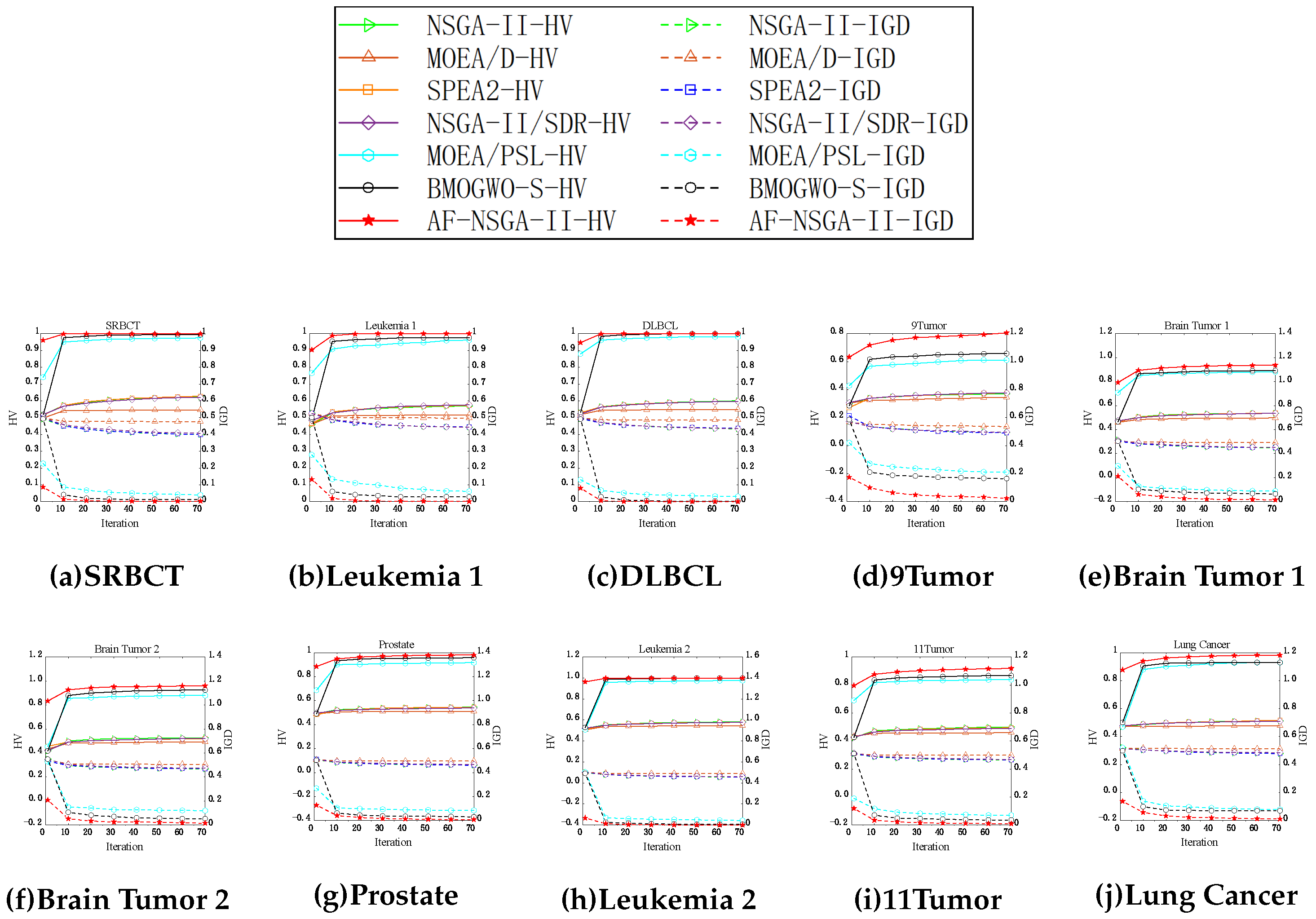
To facilitate a visual comparison of convergence performance among different algorithms, the HV and IGD convergence trajectories of seven algorithms across ten datasets have been plotted. In Figure 3, each subfigure employs a dual vertical axis system: the left vertical axis quantifies HV values while the right vertical axis calibrates IGD values, with the horizontal axis uniformly representing iteration counts. Notably, the first subfigure is a legend. In subsequent subfigures, solid lines in the upper half depict HV convergence paths, while dashed lines in the lower half illustrate IGD evolutionary trajectories. All data points were calculated by averaging results from 10 independent runs, thereby effectively mitigating the impact of random fluctuations.

By comparing the convergence curves of the NSGA-II, MOEA/D, SPEA2, NSGA-II/SDR, and BMOGWO-S, it can be observed that all five algorithms utilize a standard random initialization method, leading to similar performance characteristics in the initial stages of the algorithms. Additionally, as the initialization of MOEA/PSL is based on Latin hypercube sampling, its effect is slightly superior to that of random initialization methods. The initialization process of AF-NSGA-II not only integrates the dataset’s internal feature information, but also employs multiple filter feature selection methods for sparse initialization. Therefore, its initialization performance surpasses traditional random initialization methods across all datasets. AF-NSGA-II exhibits stronger initial HV and IGD values, and the initial solutions it yields are more proximate to the optimal Pareto solution set.

With the increase in the number of iterations from 10 to 70, it becomes evident that MOEA/PSL, AF-NSGA-II, and BMOGWO-S demonstrate faster convergence across the majority of datasets compared to other algorithms. Of these, BMOGWO-S achieves the fastest convergence; however, its HV and IGD values consistently lag behind those of AF-NSGA-II. This discrepancy is attributed to its initial solutions being farther from the optimal Pareto front. Furthermore, throughout the evolutionary process, AF-NSGA-II registers the highest HV values as well as the lowest IGD values in the majority of datasets. In summary, AF-NSGA-II exhibits rapid iterative convergence and robust search capabilities, indicating that it requires fewer iterations to approach the optimal Pareto front in high-dimensional datasets.

5.3. Analysis of Pareto Front

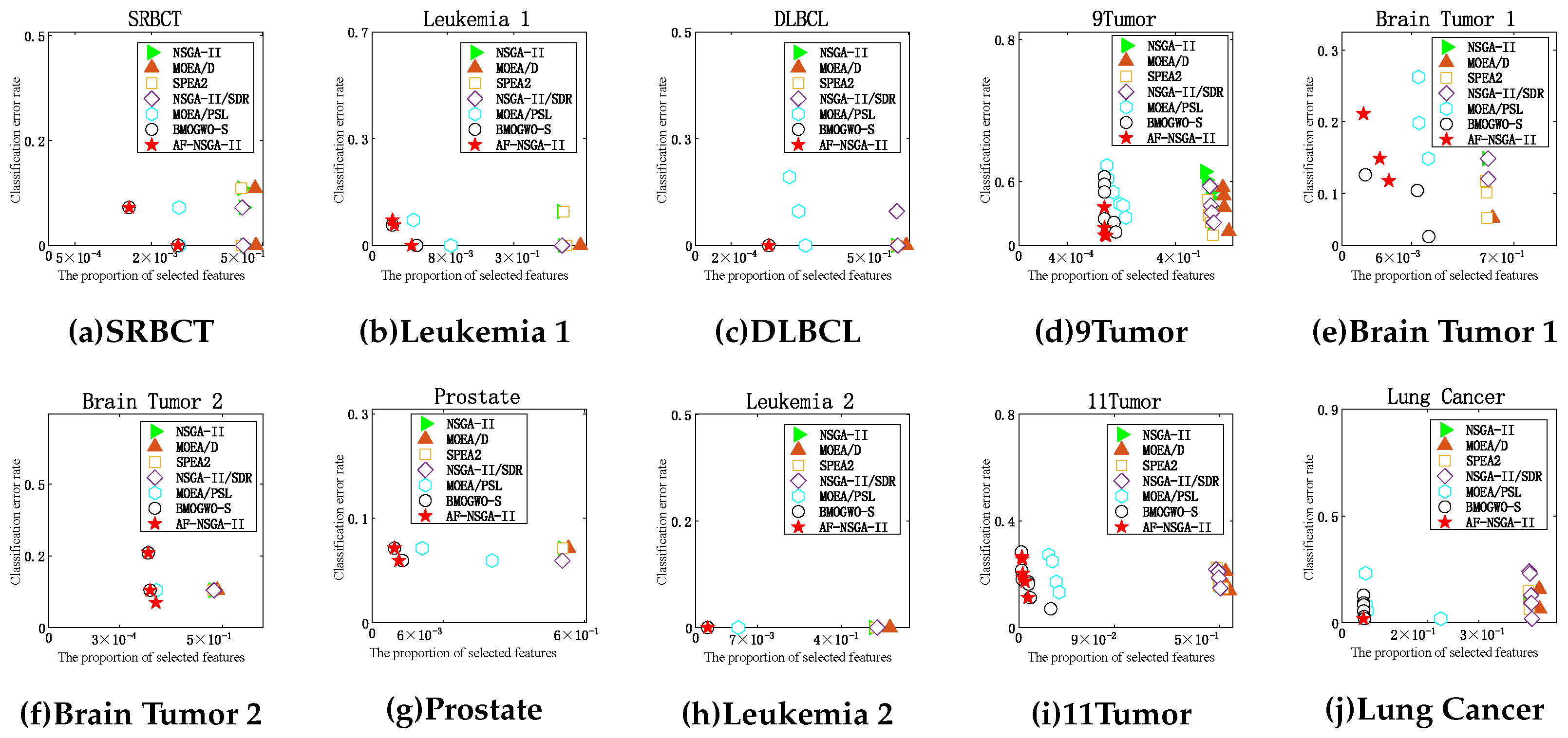
Figure 4 illustrates the distribution of Pareto fronts obtained by each algorithm across different test datasets. The Pareto front for each algorithm is derived from the outcomes of the final populations in 10 separate experimental runs.

From Figure 4, it is evident that across all datasets, AF-NSGA-II, MOEA/PSL, and BMOGWO-S achieve a significantly lower feature selection ratio in most of the feature subsets obtained, while maintaining low classification error rates when compared to the other four algorithms. This demonstrates the powerful feature reduction and error reduction capabilities of these three algorithms. Additionally, in most datasets, the solutions produced by AF-NSGA-II outperform MOEA/PSL and BMOGWO-S. Considering these observations, it can be inferred that AF-NSGA-II offers a more effective approach for addressing feature selection in high-dimensional spaces compared to the other benchmark algorithms.

5.4. Ablation Study

AF-NSGA-II employ an initialization strategy guided by multiple filter feature selection methods and an adaptive crossover mechanism based on parental similarity. Therefore, this study conducted ablation experiments to verify whether these two techniques would affect the effectiveness of AF-NSGA-II.

Initially, the proposed sparse initialization method was integrated with NSGA-II. Through this combination, a novel algorithm emerged, which was christened F-NSGA-II. Subsequently, NSGA-II was combined with the adaptive crossover operator, and the result was A-NSGA-II. Then we compared the performance of NSGA-II, F-NSGA-II, A-NSGA-II, and AF-NSGA-II across 10 datasets and evaluated their effectiveness using the HV metric. The average and standard deviation of HV values are presented in

Table 6. The mean HV values of AF-NSGA-II and ablation experiments.

No.	NSGA-II	F-NSGA-II	A-NSGA-II	AF-NSGA-II
	Mean	Mean	Mean	Mean
	(Std)W	(Std)W	(Std)W	Std
DS01	$6.39\times {10}^{-1}$	$9.38\times {10}^{-1}$	$6.96\times {10}^{-1}$	$9.98\times {10}^{-1}$
	($4.17\times {10}^{-3}$)−	($2.64\times {10}^{-4}$)−	($4.17\times {10}^{-3}$)−	$3.72\times {10}^{-5}$
DS02	$6.04\times {10}^{-1}$	$9.39\times {10}^{-1}$	$6.59\times {10}^{-1}$	$9.93\times {10}^{-1}$
	($3.85\times {10}^{-3}$)−	($2.48\times {10}^{-4}$)−	($5.19\times {10}^{-3}$)−	$1.90\times {10}^{-2}$
DS03	$6.08\times {10}^{-1}$	$9.39\times {10}^{-1}$	$6.56\times {10}^{-1}$	$9.99\times {10}^{-1}$
	($3.91\times {10}^{-3}$)−	($1.04\times {10}^{-4}$)−	($4.79\times {10}^{-3}$)−	$1.17\times {10}^{-16}$
DS04	$3.52\times {10}^{-1}$	$6.34\times {10}^{-1}$	$3.92\times {10}^{-1}$	$6.65\times {10}^{-1}$
	($3.18\times {10}^{-2}$)−	($4.66\times {10}^{-2}$)≈	($3.76\times {10}^{-2}$)−	$5.21\times {10}^{-2}$
DS05	$4.90\times {10}^{-1}$	$8.02\times {10}^{-1}$	$5.44\times {10}^{-1}$	$8.74\times {10}^{-1}$
	($2.70\times {10}^{-2}$)−	($4.71\times {10}^{-2}$)−	($2.96\times {10}^{-2}$)−	$3.54\times {10}^{-2}$
DS06	$5.15\times {10}^{-1}$	$8.40\times {10}^{-1}$	$5.72\times {10}^{-1}$	$8.74\times {10}^{-1}$
	($2.22\times {10}^{-2}$)−	($1.96\times {10}^{-2}$)−	($7.70\times {10}^{-3}$)−	$3.58\times {10}^{-2}$
DS07	$5.34\times {10}^{-1}$	$8.56\times {10}^{-1}$	$5.87\times {10}^{-1}$	$9.13\times {10}^{-1}$
	($3.70\times {10}^{-3}$)−	($7.97\times {10}^{-3}$)−	($6.77\times {10}^{-3}$)−	$7.57\times {10}^{-3}$
DS08	$5.87\times {10}^{-1}$	$9.39\times {10}^{-1}$	$6.34\times {10}^{-1}$	$9.99\times {10}^{-1}$
	($2.92\times {10}^{-3}$)−	($3.41\times {10}^{-5}$)−	($2.85\times {10}^{-3}$)−	$1.17\times {10}^{-4}$
DS09	$5.03\times {10}^{-1}$	$8.44\times {10}^{-1}$	$5.52\times {10}^{-1}$	$8.99\times {10}^{-1}$
	($2.55\times {10}^{-2}$)−	($3.11\times {10}^{-2}$)−	($2.60\times {10}^{-2}$)−	$4.95\times {10}^{-2}$
DS10	$5.23\times {10}^{-1}$	$8.91\times {10}^{-1}$	$5.84\times {10}^{-1}$	$9.43\times {10}^{-1}$
	($3.07\times {10}^{-2}$)−	($3.26\times {10}^{-2}$)−	($2.04\times {10}^{-2}$)−	$3.29\times {10}^{-2}$
+/−/≈	0/10/0	0/9/1	0/10/0

. Analysis of Table 6 reveals that A-NSGA-II consistently outperforms NSGA-II across all datasets, demonstrating the effectiveness of the adaptive crossover mechanism. In contrast, A-NSGA-II performs less effectively than both AF-NSGA-II and F-NSGA-II. This finding indicates that the sparse initialization method is not only beneficial, but also more effective than the adaptive crossover mechanism for high-dimensional feature selection tasks. Additionally, empirical observations demonstrate that the AF-NSGA-II algorithm exhibits the most superior performance across all test datasets, which further validates the efficacy of the initialization strategy and adaptive crossover mechanism proposed in this paper in addressing high-dimensional feature selection challenges.

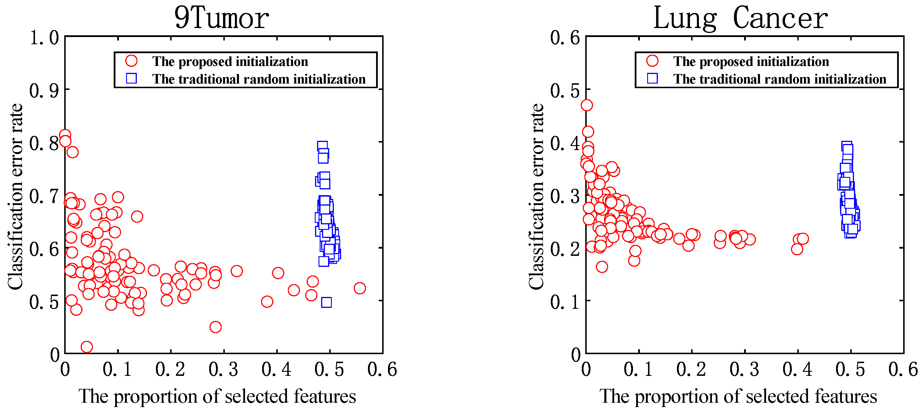
In this section, experiments were conducted to examine the distribution characteristics of the solutions generated by this strategy and those produced by the traditional random initialization strategy.

As demonstrated in Figure 5, the initial solution distributions for the 9Tumor and Lung Cancer datasets are visually contrasted under different initialization schemes, with each dataset comprising 100 candidate solutions. The conventional random initialization method assigns values to each decision variable with equal probability, resulting in a feature selection ratio in the initial population that is concentrated around 0.5. In contrast, the proposed initialization method generates initial solutions with improved convergence and diversity across different datasets, demonstrating its effectiveness.

6. Conclusions

To mitigate the issue of decreased search capability of traditional MO evolutionary algorithms when faced with a high-dimensional feature space, this study proposes a new algorithm: AF-NSGA-II, which is an improved version of NSGA-II. Specifically, it introduces a population initialization strategy guided by multiple filter feature selection methods, which accelerates convergence and reduces computational costs. Additionally, this study introduces an adaptive crossover mechanism driven by parent similarity, dynamically selecting both geometric (facilitating convergence) and non-geometric (promoting diversity) crossover operators. This ensures an effective balance between convergence and diversity. To evaluate its effectiveness, AF-NSGA-II was compared against six renowned MO evolutionary algorithms across ten publicly accessible high-dimensional datasets. The experimental outcomes revealed that AF-NSGA-II achieves superior solution sets, exhibiting better convergence and diversity on most datasets, and maintains impressive classification performance, even with reduced feature sets. Moreover, it demonstrates excellent convergence speed.

In future work, we intend to integrate variable-length encoding to further enhance the effectiveness of MO evolutionary algorithms in addressing the high-dimensional feature selection problem.

References

1. Xue, Y.; Zhu, H.; Neri, F. A feature selection approach based on NSGA-II with ReliefF. Appl. Soft Comput. 2023, 134, 109987. [Google Scholar] [CrossRef]
2. Hong, H.; Jiang, M.; Yen, G.G. Boosting scalability for large-scale multiobjective optimization via transfer weights. Inf. Sci. 2024, 670, 120607. [Google Scholar] [CrossRef]
3. Tran, B.; Xue, B.; Zhang, M. Variable-length particle swarm optimization for feature selection on high-dimensional classification. IEEE Trans. Evol. Comput. 2018, 23, 473–487. [Google Scholar] [CrossRef]
4. Yue, C.T.; Liang, J.J.; Qu, B.Y.; Yu, K.J.; Song, H. Multimodal Multiobjective Optimization in Feature Selection. In Proceedings of the 2019 IEEE Congress on Evolutionary Computation (CEC), Wellington, New Zealand, 10–13 June 2019; IEEE: Piscataway, NJ, USA, 2019; pp. 302–309. [Google Scholar] [CrossRef]
5. Liang, Z.P.; Wang, K.; Zhou, Q.; Wang, J.; Zhu, Z. Sparse large-scale multiobjective optimization based on evolutionary multitasking. Chin. J. Comput. 2025, 48, 358–380. (In Chinese) [Google Scholar] [CrossRef]
6. Zhang, Y.; Gong, D.W.; Gao, X.Z.; Tian, T.; Sun, X.Y. Binary differential evolution with self-learning for multi-objective feature selection. Inf. Sci. 2020, 507, 67–85. [Google Scholar] [CrossRef]
7. Xue, B.; Zhang, M.; Browne, W.N. Particle swarm optimization for feature selection in classification: A multi-objective approach. IEEE Trans. Cybern. 2012, 43, 1656–1671. [Google Scholar] [CrossRef] [PubMed]
8. Li, X.; Fu, Q.; Li, Q.; Ding, W.; Lin, F.; Zheng, Z. Multi-objective binary grey wolf optimization for feature selection based on guided mutation strategy. Appl. Soft Comput. 2023, 145, 110558. [Google Scholar] [CrossRef]
9. Wang, Z.; Gao, S.; Zhou, M.; Sato, S.; Cheng, J.; Wang, J. Information-Theory-based Nondominated Sorting Ant Colony Optimization for Multiobjective Feature Selection in Classification. IEEE Trans. Cybern. 2023, 53, 5276–5289. [Google Scholar] [CrossRef]
10. Wang, X.H.; Zhang, Y.; Sun, X.Y.; Wang, Y.L.; Du, C.H. Multi-objective feature selection based on artificial bee colony: An acceleration approach with variable sample size. Appl. Soft Comput. 2020, 88, 106041. [Google Scholar] [CrossRef]
11. Xue, Y.; Cai, X.; Neri, F. A multi-objective evolutionary algorithm with interval based initialization and self-adaptive crossover operator for large-scale feature selection in classification. Appl. Soft Comput. 2022, 127, 109420. [Google Scholar] [CrossRef]
12. Labani, M.; Moradi, P.; Jalili, M. A multi-objective genetic algorithm for text feature selection using the relative discriminative criterion. Expert Syst. Appl. 2020, 149, 113276. [Google Scholar] [CrossRef]
13. Purshouse, R.C.; Fleming, P.J. On the evolutionary optimization of many conflicting objectives. IEEE Trans. Evol. Comput. 2007, 11, 770–784. [Google Scholar] [CrossRef]
14. Fan, Z.; Li, W.; Cai, X.; Li, H.; Wei, C.; Zhang, Q.; Deb, K.; Goodman, E. Push and pull search for solving constrained multi-objective optimization problems. Swarm Evol. Comput. 2019, 44, 665–679. [Google Scholar] [CrossRef]
15. Jing, Q.; Guo, Y.; Liu, Y.; Wang, Y.; Du, C.; Liu, X. Optimization study of energy saving control strategy of carbon dioxide heat pump water heater system under the perspective of energy storage. Appl. Therm. Eng. 2025, 283, 129030. [Google Scholar] [CrossRef]
16. Robnik-Šikonja, M.; Kononenko, I. Theoretical and empirical analysis of ReliefF and RReliefF. Mach. Learn. 2003, 53, 23–69. [Google Scholar] [CrossRef]
17. Reshef, D.N.; Reshef, Y.A.; Finucane, H.K.; Grossman, S.R.; McVean, G.; Turnbaugh, P.J.; Lander, E.S.; Mitzenmacher, M.; Sabeti, P.C. Detecting novel associations in large data sets. Science 2011, 334, 1518–1524. [Google Scholar] [CrossRef] [PubMed]
18. Sun, L.; Wang, T.; Ding, W.; Xu, J.; Lin, Y. Feature selection using Fisher score and multilabel neighborhood rough sets for multilabel classification. Inf. Sci. 2021, 578, 887–912. [Google Scholar] [CrossRef]
19. Moraglio, A.; Poli, R. Topological Interpretation of Crossover. In Genetic and Evolutionary Computation—GECCO, Proceedings of the Genetic and Evolutionary Computation Conference, Seattle, DC, USA, 26–27 June 2004; Deb, K., Ed.; Springer: Berlin/Heidelberg, Germany, 2004; pp. 1377–1388. [Google Scholar]
20. Moraglio, A.; Poli, R. Product Geometric Crossover. In Parallel Problem Solving from Nature—PPSN IX, Proceedings of the International Conference on Parallel Problem Solving from Nature, Reykjavik, Iceland, 9–13 September 2006; Runarsson, T.P., Beyer, H.G., Burke, E., Merelo-Guervós, J.J., Whitley, L.D., Yao, X., Eds.; Springer: Berlin/Heidelberg, Germany, 2006; pp. 1018–1027. [Google Scholar]
21. Ishibuchi, H.; Tsukamoto, N.; Nojima, Y. Diversity improvement by non-geometric binary crossover in evolutionary multiobjective optimization. IEEE Trans. Evol. Comput. 2010, 14, 985–998. [Google Scholar] [CrossRef]
22. Moraglio, A.; Poli, R. Inbreeding Properties of Geometric Crossover and Non-geometric Recombinations. In Foundations of Genetic Algorithms, Proceedings of the International Workshop on Foundations of Genetic Algorithms, Mexico City, Mexico, 8–11 January 2007; Stephens, C.R., Toussaint, M., Whitley, D., Stadler, P.F., Eds.; Springer: Berlin/Heidelberg, Germany, 2007; pp. 1–14. [Google Scholar]
23. Ma, H.; Zhang, Y.; Sun, S.; Liu, T.; Shan, Y. A comprehensive survey on NSGA-II for multi-objective optimization and applications. Artif. Intell. Rev. 2023, 56, 15217–15270. [Google Scholar] [CrossRef]
24. Hamdani, T.M.; Won, J.M.; Alimi, A.M.; Karray, F. Multi-objective Feature Selection with NSGA II. In Adaptive and Natural Computing Algorithms, Proceedings of the International Conference on Adaptive and Natural Computing Algorithms, Warsaw, Poland, 11–14 April 2007; Beliczynski, B., Dzielinski, A., Iwanowski, M., Ribeiro, B., Eds.; Springer: Berlin/Heidelberg, Germnay, 2007; pp. 240–247. [Google Scholar]
25. Wang, P.; Xue, B.; Zhang, M.; Liang, J. A Grid-dominance based Multi-objective Algorithm for Feature Selection in Classification. In Proceedings of the 2021 IEEE Congress on Evolutionary Computation (CEC), Virtual, 28 June–1 July 2021; IEEE: Piscataway, NJ, USA, 2021. [Google Scholar] [CrossRef]
26. Rehman, A.U.; Nadeem, A.; Malik, M.Z. Fair feature subset selection using multiobjective genetic algorithm. In Proceedings of the Genetic and Evolutionary Computation Conference Companion, New York, NY, USA, 9–13 July 2022; GECCO ’22. pp. 360–363. [Google Scholar] [CrossRef]
27. Gong, Y.; Zhou, J.; Wu, Q.; Zhou, M.; Wen, J. A Length-Adaptive Non-Dominated Sorting Genetic Algorithm for Bi-Objective High-Dimensional Feature Selection. IEEE/CAA J. Autom. Sin. 2023, 10, 1834–1844. [Google Scholar] [CrossRef]
28. Li, M.; Ma, H.; Lv, S.; Wang, L.; Deng, S. Enhanced NSGA-II-based feature selection method for high-dimensional classification. Inf. Sci. 2024, 663, 120269. [Google Scholar] [CrossRef]
29. Jiao, R.; Xue, B.; Zhang, M. Sparse Learning-Based Feature Selection in Classification: A Multi-Objective Perspective. IEEE Trans. Emerg. Top. Comput. Intell. 2024, 9, 2767–2781. [Google Scholar] [CrossRef]
30. Vijai, P. A hybrid multi-objective optimization approach with NSGA-II for feature selection. Decis. Anal. J. 2025, 14, 100550. [Google Scholar] [CrossRef]
31. Patterson, G.; Zhang, M. Fitness Functions in Genetic Programming for Classification with Unbalanced Data. In Proceedings of the AI 2007: Advances in Artificial Intelligence, Gold Coast, Australia, 2–6 December 2007; Orgun, M.A., Thornton, J., Eds.; Springer: Berlin/Heidelberg, Germany, 2007; pp. 769–775. [Google Scholar]
32. Tian, Y.; Zhang, X.; Wang, C.; Jin, Y. An evolutionary algorithm for large-scale sparse multiobjective optimization problems. IEEE Trans. Evol. Comput. 2019, 24, 380–393. [Google Scholar] [CrossRef]
33. Xue, Y.; Zhu, H.; Liang, J.; Słowik, A. Adaptive crossover operator based multi-objective binary genetic algorithm for feature selection in classification. Knowl.-Based Syst. 2021, 227, 107218. [Google Scholar] [CrossRef]
34. McGinley, B.; Maher, J.; O’Riordan, C.; Morgan, F. Maintaining healthy population diversity using adaptive crossover, mutation, and selection. IEEE Trans. Evol. Comput. 2011, 15, 692–714. [Google Scholar] [CrossRef]
35. Pan, H.; Chen, S.; Xiong, H. A high-dimensional feature selection method based on modified Gray Wolf Optimization. Appl. Soft Comput. 2023, 135, 110031. [Google Scholar] [CrossRef]
36. Zhou, Y.; Zhang, W.; Kang, J.; Zhang, X.; Wang, X. A problem-specific non-dominated sorting genetic algorithm for supervised feature selection. Inf. Sci. 2021, 547, 841–859. [Google Scholar] [CrossRef]
37. Xu, H.; Xue, B.; Zhang, M. A duplication analysis-based evolutionary algorithm for biobjective feature selection. IEEE Trans. Evol. Comput. 2020, 25, 205–218. [Google Scholar] [CrossRef]
38. Deb, K.; Pratap, A.; Agarwal, S.; Meyarivan, T. A fast and elitist multiobjective genetic algorithm: NSGA-II. IEEE Trans. Evol. Comput. 2002, 6, 182–197. [Google Scholar] [CrossRef]
39. Zitzler, E.; Laumanns, M.; Thiele, L. SPEA2: Improving the Strength Pareto Evolutionary Algorithm; TIK Report; Technical Report No. 103; Computer Engineering and Networks Laboratory: Zurich, Switzerland, 2001. [Google Scholar]
40. Zhang, Q.; Li, H. MOEA/D: A multiobjective evolutionary algorithm based on decomposition. IEEE Trans. Evol. Comput. 2007, 11, 712–731. [Google Scholar] [CrossRef]
41. Tian, Y.; Cheng, R.; Zhang, X.; Su, Y.; Jin, Y. A strengthened dominance relation considering convergence and diversity for evolutionary many-objective optimization. IEEE Trans. Evol. Comput. 2018, 23, 331–345. [Google Scholar] [CrossRef]
42. Tian, Y.; Lu, C.; Zhang, X.; Tan, K.C.; Jin, Y. Solving Large-Scale Multiobjective Optimization Problems With Sparse Optimal Solutions via Unsupervised Neural Networks. IEEE Trans. Cybern. 2021, 51, 3115–3128. [Google Scholar] [CrossRef] [PubMed]
43. Al-Tashi, Q.; Abdulkadir, S.J.; Rais, H.M.; Mirjalili, S.; Alhussian, H.; Ragab, M.G.; Alqushaibi, A. Binary Multi-Objective Grey Wolf Optimizer for Feature Selection in Classification. IEEE Access 2020, 8, 106247–106263. [Google Scholar] [CrossRef]
44. Zitzler, E.; Thiele, L.; Laumanns, M.; Fonseca, C.M.; Da Fonseca, V.G. Performance assessment of multiobjective optimizers: An analysis and review. IEEE Trans. Evol. Comput. 2003, 7, 117–132. [Google Scholar] [CrossRef]
45. While, L.; Hingston, P.; Barone, L.; Huband, S. A faster algorithm for calculating hypervolume. IEEE Trans. Evol. Comput. 2006, 10, 29–38. [Google Scholar] [CrossRef]
Figure 1. Non-Geometric crossover operator.
Electronics 15 00236 g001
Figure 2. Example of adaptive crossover based on parental similarity.
Electronics 15 00236 g002
Figure 3. Convergence curves of seven algorithms.
Electronics 15 00236 g003
Figure 4. Pareto fronts of seven algorithms.
Electronics 15 00236 g004
Figure 5. The initial populations’ distribution of the 9Tumor and Lung Cancer datasets (i.e., 9Tumor and Lung Cancer in Table 1).
Electronics 15 00236 g005