Automatic Pruning and Quality Assurance of Object Detection Datasets for Autonomous Driving

Abstract

Large amounts of high-quality data are required to train artificial intelligence (AI) models; however, curating such data through human intervention remains cumbersome, time-consuming, and error-prone. In particular, erroneous annotations and statistical imbalances in object detection datasets can significantly degrade model performance in real-world autonomous driving scenarios. This study proposes an automated pruning framework and quality assurance strategy for 2D object detection datasets to address these issues. The framework is composed of two stages: (1) noisy label identification and deletion based on labeling scores derived from the inference results of multiple object detection models, and (2) statistical distribution whitening based on class and bounding box size diversity metrics. The proposed method was designed in accordance with the ISO/IEC 25012 data quality standards to ensure data consistency, accuracy, and completeness. Experiments were conducted on widely used autonomous driving datasets, including KITTI, Waymo, nuScenes, and large-scale publicly available datasets from South Korea. An automated data pruning process was employed to eliminate anomalous and redundant samples, resulting in a more reliable and compact dataset for model training. The results demonstrate that the proposed method substantially reduces the amount of training data required, while enhancing the detection performance and minimizing manual inspection efforts.

1. Introduction

Artificial intelligence (AI) technology has rapidly developed, achieving remarkable results in fields such as autonomous driving [1,2], and healthcare [3]. These advances require four key elements: the model, data, hardware, and software. High-performance hardware leverages data and software to create AI models and efficiently train them. To improve AI models further, experts have emphasized the importance of large amounts of high-quality data [4,5,6]. These processed data play a crucial role in effectively training the AI models. The amount of high-quality data required for training AI models is a significant factor in yielding reliable AI models. These data, which serve as inputs for the model training, should be free of anomalies. Data labeling is typically performed to generate large datasets, such that human operators with basic knowledge and experience in data processing are required. However, manual labeling has limitations in terms of the number of available operators and unforeseen human errors. Additionally, differences in workers’ backgrounds and expertise can lead to biases and anomalies.

Developing a systematic method to enhance data quality is essential. The ISO/IEC 25012 [7] standard, as well as the “Data Quality Management Guidelines for AI Training” [8] published by the Korean Ministry of Science and the National Information Society Agency, provide procedures and principles for managing and evaluating data quality. The “Data Quality Model” measures the level of data quality and is categorized into six main categories: accuracy, completeness, consistency, reliability, validity, and expressiveness. A study [9] highlighted the importance of quality verification in ensuring the reliability and validity of data by focusing on quality assurance using standards. Another study [10] utilized an ontology-based method to evaluate data quality according to standards, and established metrics for functionality and reliability. A previous study [11] demonstrated the use of metrics derived from standards to assess and enhance the quality of data.

Model-centric methods that optimize model structure and function have been used to improve the performance and reliability of AI models [12,13]. Some studies have proposed new loss functions to minimize the effect of noisy labels and train noise-robust models [14,15,16,17]. However, changing the model structure could solve certain problems. Therefore, data-centric methods are essential [18,19] for efficient data collection, classification, pruning, and processing to construct training datasets [20,21,22]. There are studies on Noisy Label Learning (NLL) [23,24,25] that aimed to improve the generalization performance of models using training data with noisy labels, rather than overcoming noisy data. These studies have proposed introducing new types of noise or methods to distinguish challenging data. Flawed data can degrade the performance of AI model training or cause erroneous results [26,27,28]. A previous study [29] outlined the training of deep learning models with noisy labels and presented a method for correcting label noise. Similarly, data preprocessing, such as removing or correcting data with anomalies, is required [30,31].

Previous studies have investigated the importance of datasets in training models [32]. The authors proposed a cross-validation framework using various convolutional neural networks (CNNs) to validate data quality and efficiency. Focusing on label correlation, another study [33] proposed a method to enhance multi-label annotation using noisy crowdsourced data. A framework [34] for identifying and correcting noisy labels in crowdsourced labeled datasets also exists. Several correction algorithms [35,36] have been proposed to address noise interference when datasets containing noisy labels are used. These algorithms use a consensus voting method to solve the noisy label problem. A label enhancement method [37] was developed to refine label distributions and improve the classification performance in noisy datasets by utilizing trusted data. Several studies [38,39,40,41,42] have adopted active learning as a model-training strategy to iteratively improve the model performance by reconstructing data. Effective relabeling through prioritization can improve dataset quality.

In a practical training dataset, it is essential to ensure that each label is unbiased and that there are no duplicate data. If models are trained on biased datasets, they may not perform well on other test sets. Therefore, methods such as data preprocessing or exclusion should be employed during training [43,44,45]. One study [46] computed the density from the class distribution of objects in redundant data by selecting the best data sample for model training. Some studies [47,48,49] investigated the correlation between data quality and AI model performance using data quality assessments. One study [48] used a machine learning model to check label quality in an object detection project. A small high-quality dataset was reprocessed from one that required quality validation and trained using a neural network for quality validation. One study [50] focused on selecting optimal instances from datasets with imperfect labels, and proposed algorithms that prioritize data subsets based on their expected labeling quality.

2. Methodology

In this study, we propose an automated process to ensure the quality of autonomous driving (AD) datasets for 2D object detection AI models by removing outlier data and normalizing the distribution. As shown in Figure 1, a framework is introduced that prevents contamination by anomalous data and enables effective learning by eliminating redundancies and bias. The first step involves discarding noisy labels. A labeling score was introduced that employs inference results from multiple AI models to evaluate data anomalies. The noisy labels are filtered based on inter-model consistency, without requiring human intervention. Subsequently, the data distribution is whitened. The diversity scores were calculated by comprehending the class and bounding box size distributions. Using these scores, data priorities are determined, and less informative or redundant data are removed, forming an assurance dataset automatically. Based on these scores, the system prioritizes the data and proceeds with data reduction.

In this study, a dataset pruning process was used to remove abnormal data from the dataset and to whiten the distribution. Thus, automated quality assurance was executed through the utilization of an AI model rather than manual examination, thereby achieving the following technical benefits.

• Automated quality assurance of the AI training dataset.
• Calculation of data quality indicators through prediction results of the trained model.
• Calculation of statistical indicators to satisfy statistical diversity and eliminate bias.
• Reducing the amount of data required for training.
• Automatic classification of data requiring re-annotating.

The remainder of this paper is organized as follows. Section 3 describes the deletion of noisy labels and automatic detection and removal of abnormal data. Section 4 describes the process of whitening the data distribution, wherein the data are reduced based on the distribution. Section 5 provides both qualitative and quantitative outcomes, showing the enhancement in the performance of the model resulting from the eradication of noisy labels and distribution whitening. Section 6 analyses the overall experimental outcomes of the study and their influence on the subsequent research practices in the field and Section 7 concludes this research study.

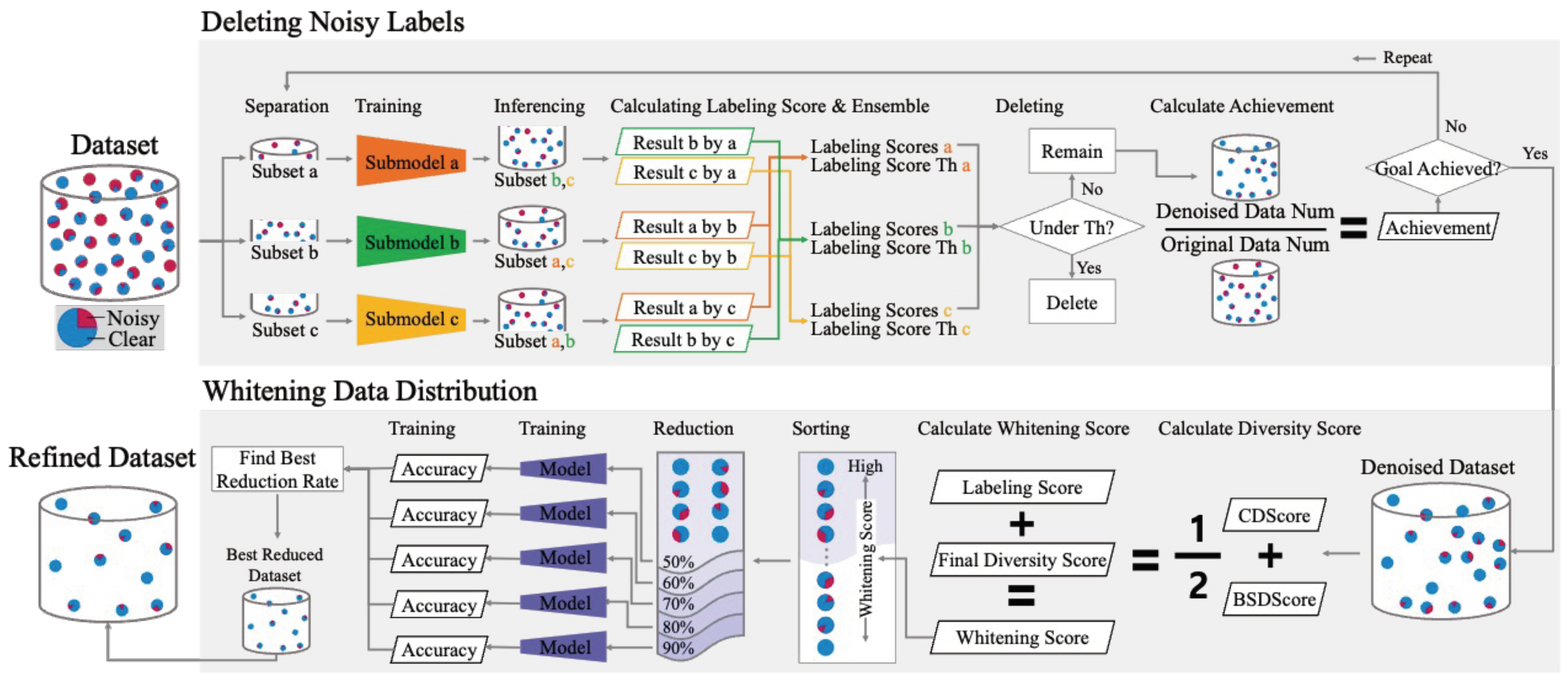
3. Proposed System: Deleting Noisy Labels

3.1. Overview

The first step in this study involves identifying and deleting noisy data, as shown in Figure 2. To demonstrate this process, we provide examples of both clean and noisy labels across the six datasets used in the investigation. The first column illustrates the ideal scenario with precise annotations. The second column contains samples in which the objects are either misclassified or have misaligned bounding boxes. The third column presents bounding boxes that are either excessively large or insufficiently small to enclose the target object adequately. The fourth column displays instances in which an anticipated label is absent. The final column includes corrupted data resulting from issues in the label files such as unreadable or invalid annotations.

To guarantee the quality of the AI datasets, several institutions perform visual inspections to verify the data for errors or inaccuracies. However, this procedure requires human intervention, and examining the entire dataset is challenging, time consuming, and costly. Our research project trained several models that automatically filtered noisy labels and employed them to identify and rectify anomalous data in an entire dataset. As depicted in Figure 3, the process of deleting noisy labels proceeds in three stages: model training, ensemble labeling scoring, and deletion. The ensemble labeling score determines the data to be deleted and retained. The deletion phase computes the deletion achievement to determine whether to repeat or terminate the noisy label deletion process. This process was repeated until $95\%$ of the guidelines were met [8].

3.2. Defining LScore

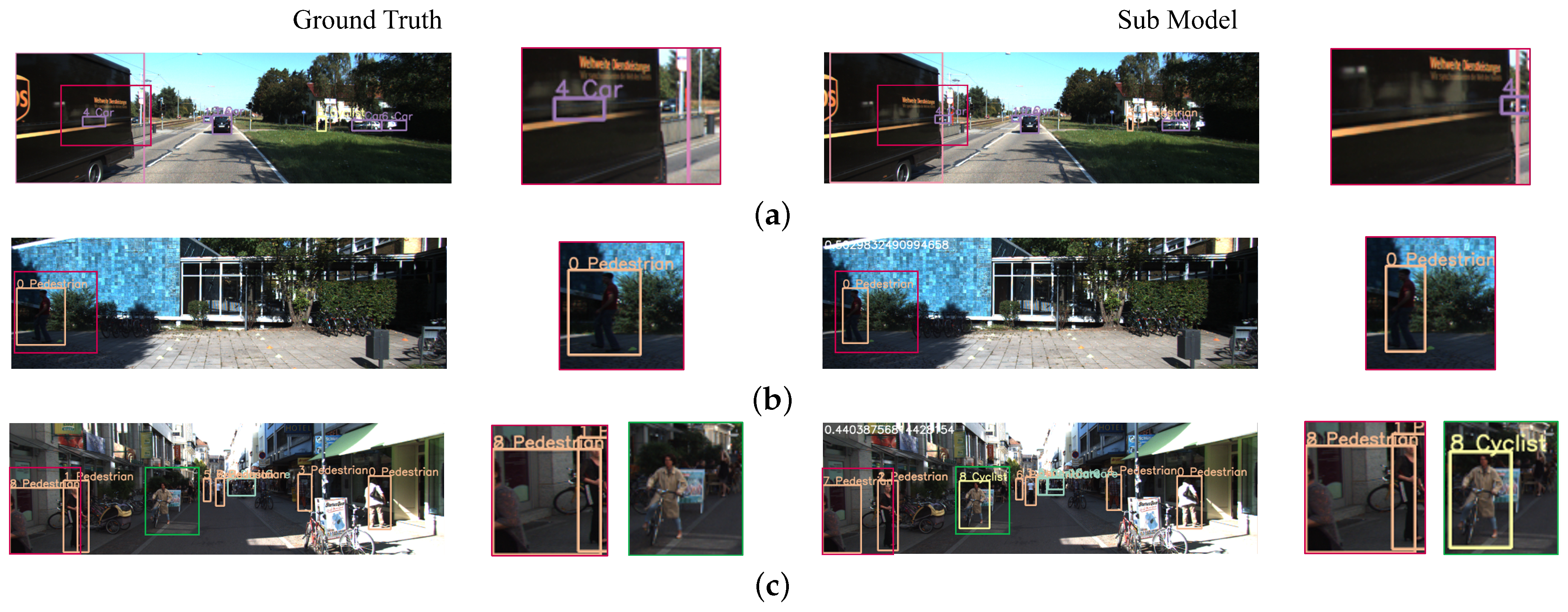
In this study, a “Labeling Score (LScore)” was defined to automatically detect noisy data. The ISO/IEC 25012 standard outlines characteristics for assessing data quality independently of specific systems or environments. LScore is based on the indicators of accuracy, completeness, and credibility, which are used as data quality verification indicators. Accuracy measures how well data represent actual values and uses the intersection over union (IoU) metric to calculate the overlap between model-influenced and GT bounding boxes for each object in the frame. Completeness verifies the inclusion of all expected instances and is ensured through recall, an activation function that ensures all valid objects in a frame are labelled. Credibility evaluates data trustworthiness from the user’s perspective and is verified via the confidence score, which represents the precision of a model’s inference for each entity in a frame. Each object in the generated dataset is evaluated to determine whether the label is correct for the class.

These three indicators collectively allow LScore to reflect the different dimensions of annotation quality. IoU-based accuracy detects spatial misalignments in object labeling, recall identifies missing annotations that degrade dataset completeness, and low-confidence scores capture uncertain or ambiguous predictions. Together, these metrics provide a quantitative basis for identifying noisy labels in accordance with ISO/IEC 25012 quality attributes of accuracy, completeness, and credibility.

3.3. Model Training

There is a process for the inspector to complete the correct answer sheet to ensure GT. In this study, the prediction results of the 2D object detection model were used. Detectron2 [51], a PyTorch 1.8.1-based object detection library, was used for efficient training. Submodels a, b, and c based on Faster R-CNN [52] with similar performances (R101-C4, R101-DC5, and R101-FPN) were trained. An evaluation model, RPN R101-FPN, was trained based on RPN and Fast R-CNN [53]. Hyperparameters were slightly adjusted from the default values provided by the Detectron2 library to fit the experimental environment, with a learning rate of $0.01$, a batch size of 8, and 5000 iterations. The trained submodels a, b, and c were used for ensemble LScores. The evaluation model was used to evaluate the performance of the remaining dataset after deleting the erroneous data. From each dataset, 20% of the data were fixed as the validation set, and the remaining 80% were split into three equal subsets for training. Submodels a, b, and c used a randomly split subset of the dataset with a 33:33:34 ratio. Repeated noisy label deletion was used to compute the LScore threshold for the initial validation dataset. The dataset did not change, but the model was iteratively trained to gradually remove noise and improve performance. Therefore, we used the score threshold of the initial validation dataset to remove the noisy labels.

3.4. LScore Ensemble

In this step, LScores are ensembled to automatically detect noisy labels and proceed with their deletion. The submodels trained on separate subsets of data, namely, a, b, and c, were verified on their respective validation datasets to determine the threshold for the LScores. Using the computed LScores and thresholds, a decision was made to retain and remove the data.

3.4.1. Calculation of the E’LScore Threshold

The E’LScore (Ensembled Labeling Score) Threshold is a criterion used for the automatic detection of noisy data. If the LScore calculated for the training dataset did not exceed the threshold, the data were considered noisy and were removed. The threshold itself is based on the averaged LScore, making it a value optimized to the dataset. By using a dataset-defined threshold, comparisons are made against values internal to the dataset, ensuring that the threshold is specifically aligned with the dataset’s characteristics.

LScore: It is a numerical measure of the quality of each frame. This is defined as a mathematical value that combines accuracy, precision, and recall. Accuracy is based on the IoU between the GT and the inferred bounding box. Precision is determined by the confidence score for the classified bounding box class, and recall is calculated based on the true-positive results. To represent the dataset inferred by the trained model, $f_{subset}$ is defined as the submodel, and ${\theta }_{sub}$ represents the parameters used in training submodel $f_{subset}$. The inference results for the validation dataset of subset are expressed as $\widetilde{{\mathrm{d}}_{\mathrm{subset}}}=f_{subset}({\theta }_{sub},d_{sub})$. The labeling score $LScor{e}_{d_i}$ is calculated using Equation (1):

$$LScor{e}_{d_i}={\displaystyle \frac{1}{n_{d_i}}}\sum _{j=0}^{N_{bo{x}_{subset}}}{w}_j\times P\left(w_j\right),$$

(1)

where the weight $w_j(j\in 0,\dots ,N_{bo{x}_{subset}})$ of each bounding box satisfies the condition $P\left(w_j\right)$ defined in Equation (2):

$$P\left(w_j\right)=[IoU(bo{x}_j,g{t}_j)\ge Io{U}_{th}\&Clas{s}_j=TP]$$

(2)

and $N_{bo{x}_{subset}}(bo{x}_{subset}\in \widetilde{d_{subset}})$ is the number of bounding boxes predicted by the submodel, with weights calculated according to Equation (3):

$$w_j=\mathrm{IoU}\left({\mathrm{box}}_j,{\mathrm{gt}}_j\right)\times {\mathrm{Conf}}_j,j\in 0,\dots ,N_{bo{x}_{subset}}.$$

(3)

$N_{subset}$ is the total number of data constituting the subset and $LScor{e}_{d_i}$ is the average LScore calculated for the $ith$ data $d_i(i\in 0,\dots ,N_{subset})$. The average value is obtained by dividing the sum of $w_j$ by the number of bounding boxes that satisfy the condition. The number of bounding boxes that satisfy this condition is denoted by $n_{d_i}$. E’LScore Threshold: This is the process of obtaining the LScores for all frames of the validation dataset of each subset and ensembling the $Avg{E}^{\prime }LScor{e}_{subset}$, the average LScore. $E^{\prime }LScoreT{h}_{subset}$ is obtained using Equation (4):

$$E^{\prime }LScoreT{h}_{subset}={\displaystyle \frac{1}{N_{subsets}-1}}\sum _{s\in \left\{a,\dots ,N_{subsets}\right\},s\ne subset}Avg{E}^{\prime }LScor{e}_s,$$

(4)

where $N_{subsets}$ represents the number of submodels. This was the average of the mean LScores of the other submodels, excluding one submodel. The E’LScore Threshold is determined dynamically as the mean value of the LScore distribution derived from cross-validated models. This approach enables the threshold to be adjusted to the statistical characteristics of each dataset, thereby avoiding reliance on a fixed heuristic. Given that LScore inherently represents the model consensus across the dataset, its average serves as a stable reference point for identifying anomalous samples, even when faced with varying dataset configurations or model ensembles.

3.4.2. Calculation of the E’LScore

By combining the inference results of the models, the E’LScore was used as a criterion for voting among the cross-validation methods. For a certain dataset, the average value was derived by calculating the LScore for each datum by inference using a model trained with another subset. E’LScore: The E’LScore follows the same approach as that described in Section 3.4.1—the ensemble labeling score threshold. For a different submodel, the LScore for each frame in the training dataset is denoted by $LScor{e}_{d_i}^{subse{t}^{\prime }}$, which corresponds to the number of bounding boxes predicted by the submodel for the frame. Each bounding box in $N_{bo{x}_{subset}^{subse{t}^{\prime }}}(bo{x}_{subset}^{subse{t}^{\prime }}\in \widetilde{d_{subset}^{subse{t}^{\prime }}})$ is associated with its weight $w_j(j\in 0,\dots ,N_{bo{x}_{subset}^{subse{t}^{\prime }}})$, which satisfies the condition in (2) $P\left(w_j\right)$. The E’LScore combines the LScores obtained from the different submodels for the same training dataset. Thus, for the $ith$ datum $d_i$ from $i=0$ to $i=N_{subset}$, the average LScore $E\text{’}LScor{e}_{d_i}^{subset}$ calculated for each frame is combined and averaged as described in (5):

$$E\text{’}LScor{e}_{d_i}^{subset}={\displaystyle \frac{1}{N_{subsets}-1}}\sum _{s\in \left\{a,b,\dots ,N_{subsets}\right\},s\ne subset}LScor{e}_{d_i}^s.$$

(5)

The combined E’LScore was used as the final comparison score for noisy label deletion.

3.5. Deleting Ratio Score

The dataset was refined by automatically detecting and deleting abnormal data by comparing the ensemble label score with the E’LScore threshold. The data to be deleted are labeling errors or missing labeling data and data that do not help in training by acting as noise in the learning process. According to condition P$\left(d_i\right)$ specified in (6),

$$P\left(d_i\right)=E\text{’}LScor{e}_{d_i}^{subset}\ge E^{\prime }LScoreT{h}_{subset},$$

(6)

the remaining data and the data to be deleted were determined for the training dataset of each subset. The dataset was then refined and organized based on (7):

$$\mathrm{for}\mathrm{all}{d}_i\mathrm{in}{N}_{subset},\left\{\begin{array}{cc}\mathrm{Maintain},\hfill & P\left(d_i\right)=\mathrm{True}\hfill \\ \mathrm{Delete},\hfill & P\left(d_i\right)=\mathrm{False}\hfill \end{array}\right..$$

(7)

During each iteration of the noisy label deletion process, the deletion achievement was calculated to achieve the recommended criterion for a semantic accuracy of 95%, according to [8]. Specifically, suppose that the proportion of data marked for deletion is 95% or higher relative to the original data quantity before the noisy label deletion process. In this case, the noisy label deletion process is halted. Finally, the remaining data, excluding the deleted data, were utilized in the data distribution whitening step. The deletion process was quantified using the deletion ratio, as shown in (8),

$$\mathrm{Deleting}\mathrm{Ratio}={\displaystyle \frac{{(N}_{Original}-N_{Deleted})}{{\mathrm{N}}_{\mathrm{Original}}}}\times 100\left(\%\right),$$

(8)

which calculates the ratio of the data count after deletion to that before deletion.

4. Proposed System: Data Distribution Whitening

4.1. Overview

Data distribution whitening balances the distribution of the classes and sizes of the objects in a dataset. It is important to consider the quantity and proportion of value objects for training. The whitening score quantifies the semantic concepts of standards and guidelines to identify statistical variability and reconstruct unbiased data. The data distribution whitening process consisted of three main steps: diversity score calculation, data whitening, and model training. These steps are executed in the order shown in Figure 4. The diversity scores comprise the scores for the class and bounding box size distributions. The final whitening score was calculated by integrating the previously used $E\text{’}LScore$ as a bias value for noisy label deletion. The data were sorted by whitening score, and low-priority data were excluded from the training dataset when training the model.

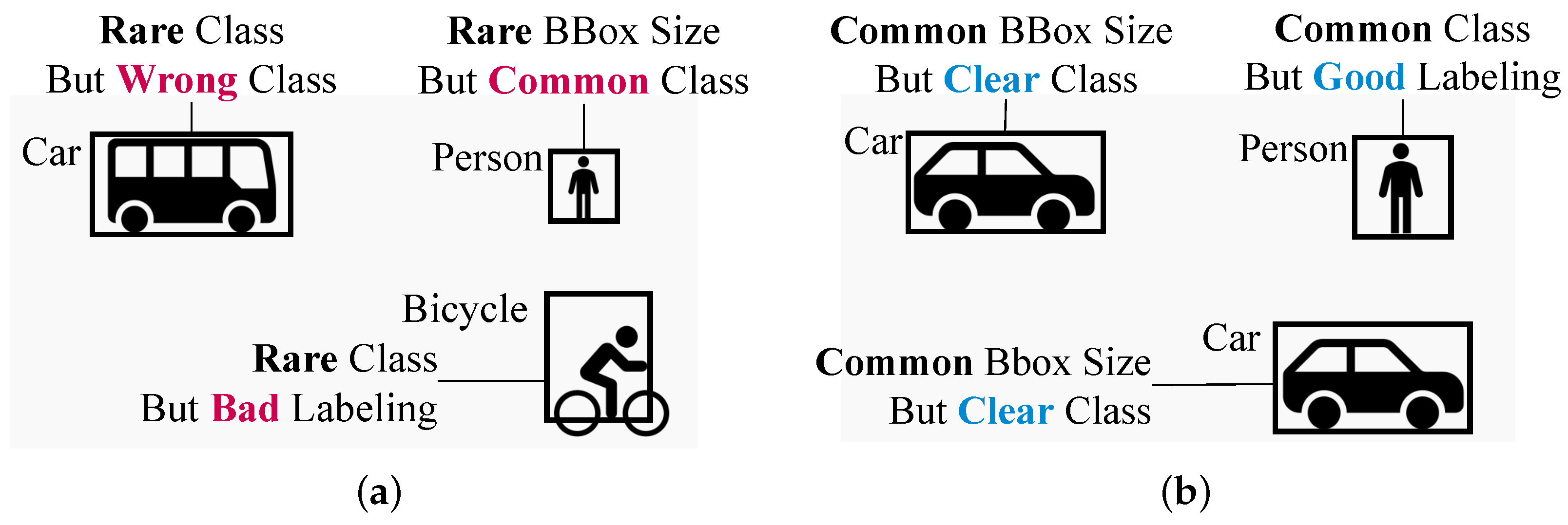
4.2. Diversity Score

The diversity score indicates the rarity of the classes of objects that comprise each frame and the object sizes. Class distribution is the number of bounding boxes that belong to each class in the dataset. The bounding box size distribution describes the size distribution of the bounding boxes that comprise all frames in the dataset. The bounding box was divided into specific ranges from the minimum to the maximum size, and the number of bounding boxes in each range was counted. Diversity scores use z-scores, also known as standard scores, which use standard deviations and variances. A negative z-score for a small data distribution indicates a below-average occurrence, while a positive z-score for a wide distribution signifies an above-average occurrence. This polarity shows the frequency of each data point relative to the mean. Reversing the z-score sign assigns higher values to rare objects, emphasizing their uniqueness. This method highlights infrequent data points, enabling the model to better identify and prioritize rare objects during training.

4.2.1. Calculation of the CDScore

The “Class Diversity Score (CDScore)” indicates that the standard score obtained for each item in the class distribution was calculated and averaged over all the bounding boxes in the frame. The class distribution list was created by counting the classes of labeled objects constituting the frame for each frame of the entire dataset. In dataset $\tilde{D}$, after deleting noisy labels, the number $x_k$ of objects belonging to class k in dataset $\tilde{D}$ is the total number of $\left({bbox}_j,y_j\right)$ pairs, where ${label}_j$ is k. The distribution list $X_{class}$, is expressed as follows in (9):

$$X_{class}=\left\{\left(k_1,x_{k_1}\right),\dots ,\left(k_{N_{class}},x_{k_{N_{class}}}\right)\right\},$$

(9)

and the class distribution list is composed of pairs of each class $k_i$ and number of objects belonging to class $x_{k_i}$.

Utilizing the class distributions obtained in (9), we generated a list of mean values, variances, standard deviations, and deviations from the distribution. Algorithm 1 is a function that receives a distribution list, normalization, and the number of distribution items as input, and returns a normalized standard deviation and a deviation list, where each item’s deviation value is multiplied by $-1$. In the algorithm, norm_list ← [0] × cnt_factor is used to initialize a list called norm_list with a length of cnt_factor, where all elements are set to 0. These values are necessary for calculating the CDScores.

Algorithm 1 Normalized Deviation List Generator

function calc_std_deviation (list, cnt_factor, norm_factor)       cnt_sum ← 0       for i ← 0 to cnt_factor $-1$ do            cnt_sum ← cnt_sum + list[i]       avg ← cnt_sum / float(cnt_factor)       avg ← avg / float(norm_factor)       norm_list ← [0] × cnt_factor       for i ← 0 to cnt_factor $-1$ do            norm_list[i] ← float(list[i]) / float(norm_factor)       dev_sum ← 0       dev_list ← [0] × cnt_factor       for i ← 0 to cnt_factor −1 do            dev ← norm_list[i] − avg            dev_sum ← dev_sum + pow(dev, 2)            dev_list[i] ← dev × − 1       var ← float(dev_sum) / float(cnt_factor)       std_var ← sqrt(var)       return std_var, dev_list

After normalizing the distribution list, the variance ${\sigma }_{class}^2$ is obtained as shown in (10):

$${\sigma }_{class}^2={\displaystyle \frac{1}{N_{class}}}\sum _{i=1}^{N_{class}}{\left(x_{k_i}-{\mu }_{class}\right)}^2.$$

(10)

The distribution value $x_{k_i}\in X_{class}$ for $N_{class}$ items is the number of items in each distribution type, and the average value is ${\mu }_{class}$. The deviation is the difference between the distribution value and the average, and the value divided by the standard deviation is the z-score, as shown in (11):

$$z_{clas{s}_i}={\displaystyle \frac{x_{k_i}-{\mu }_{class}}{{\sigma }_{class}}},i\in 0,\dots ,N_{class}.$$

(11)

In the CDScore calculation, class z-scores corresponding to the bounding boxes constituting the frame were added and averaged. To accomplish this, we used $Z_{class}$, which lists the z-scores of each item in the class distribution.

The CDScore (12) is calculated for each data point $d_i$, where $i\in 0,\dots ,N_{dataset}$ in dataset $\tilde{D}$ after noisy labels have been removed, using the following equation:

$$di{v}_{clas{s}_i}={\displaystyle \frac{1}{N_{i_{bbox}}}}\sum _{j=0}^{N_{i_{bbox}}}{Z}_{class}\left[labe{l}_j\right].$$

(12)

For all bounding boxes $bbo{x}_j$ from $j=0$ to $j=N_{i_{bbox}}$ labeled as $d_i$, the bounding box class is $labe{l}_j$. The z-score of the bounding box takes a value corresponding to the corresponding class $labe{l}_j$ from $Z_{class}$. For all bounding boxes, the value obtained by adding all elements of $Z_{class}$ corresponding to $labe{l}_j$ and averaging was calculated as the CDSCore of the corresponding data $d_i$. All bounding boxes are treated equally in this calculation, with no weighting applied.

4.2.2. Calculating BSDScore

The “Bounding box Size Diversity Score (BSDScore)” is the average of the standard scores obtained for each item in the bounding box distribution. The bounding box size distribution measures the size of all the bounding boxes in a dataset. A standard score was derived by classifying the range from the minimum to maximum size into five intervals of 20% each. The bounding box size r is defined by dividing the minimum bounding box size $s_{min}$ by the maximum bounding box size $s_{max}$ into five intervals, as shown in (13):

$$r={\displaystyle \frac{s_{max}-s_{min}}{4}}\times \left(i+1\right)fori=0to4.$$

(13)

In dataset $\tilde{D}$, $x_r$, that is, the number of objects belonging to the bounding box size r, is the number of all $\left({bbox}_j,{size}_j\right)$ pairs, where ${size}_j$ is r. The distribution list $X_{bbox\_size}$ based on this definition is represented in (14):

$$X_{bbox\_size}=(r_1,x_{r_1}),\dots ,(r_{N_{bbox\_size}},x_{r_{N_{bbox\_size}}}).$$

(14)

Using the bounding box size distribution list obtained from (14), the standard deviation and deviation lists are derived using Algorithm 1. A z-score was calculated for each bounding box size interval to derive the list $Z_{bbox\_size}$ obtained using the following Equation (15):

$$Z_{bbox\_size}=\left[z_{bbox\_siz{e}_1}={\displaystyle \frac{x_{r_1}-{\mu }_{bbox\_size}}{{\sigma }_{bbox\_size}}},\dots \right].$$

(15)

To obtain the BSDScore for one data point, the value is obtained by adding all $z_{bbox\_siz{e}_j}$ elements of $Z_{bbox\_size}$ corresponding to $siz{e}_j$ and averaging the value of the corresponding data $d_i$. The BSDScore, $di{v}_{bbox\_siz{e}_i}$, is calculated using (16), as follows:

$$di{v}_{bbox\_siz{e}_i}={\displaystyle \frac{1}{{N_i}_{bbox}}}\sum _{j=0}^{N_{i_{bbox}}}{Z}_{bbox\_size}\left[siz{e}_j\right].$$

(16)

Diversity scores were formulated to address the underrepresentation of object classes and sizes frequently encountered in complex real-world driving datasets. For instance, large vehicles, such as buses, and small objects, such as traffic cones or pedestrians, although not commonly occurring, are crucial for ensuring safety and enhancing model robustness. By identifying and prioritizing these statistically infrequent elements, the proposed method maintains the dataset coverage of semantically and spatially diverse driving scenarios, which is vital for generalization in autonomous driving applications.

4.3. Calculating the Whitening Score

Data whitening is used to measure the statistical diversity of a dataset and to adjust for imbalances in the data. This process sorts the data to prioritize the data to be reduced. Data with a low priority were excluded from the dataset based on the reduction rate. The data were reduced by 10% from the initial 100%, and the difference in performance according to the whitening score was analyzed. The RPN R101-FPN model based on a Fast R-CNN was used as the evaluation model. This was used to determine the optimal degree of reduction by comparing the performance of the models after the reduction.

The CDScore was combined with the BSDScore. The E’LScore is used to detect noisy labels and represents the bias value. The whitening score for data $d_i$, where $i\in 0,\dots ,N_{dataset}$, included in dataset $\tilde{D}$, from which the noisy labels were deleted, is calculated as shown in (17):

$$di{v}_{fina{l}_i}=(0.5\times di{v}_{clas{s}_i})+(0.5\times di{v}_{bbox\_siz{e}_i})$$

(17)

The final diversity score, $di{v_{final}}_i$, was obtained by multiplying each diversity score (CDScore and BSDScore) by $0.5$ and then adding them together. This weighting with $0.5$ represents the equal contribution of each score to the final diversity score. Priority was given to the data based on the whitening score for the final data whitening task. The whitening score in (18) is as follows:

$$Whitenin{g}_{d_i}=di{v}_{fina{l}_i}+E^{\prime }LScor{e}_{d_i},$$

(18)

and $E^{\prime }LScor{e}_{d_i}$ from (5) were added as the bias values.

The E’LScore (5) from Section 3 was used to calculate the whitening score. There were also data points with low diversity scores. These data are not sparse in terms of class or object size. However, training a model using immature data is beneficial. Only the GT was used for the diversity score calculation. The E’LSCore is necessary because it does not include judgments on whether it benefits learning. Figure 5 shows the necessity of combining E’LScores. Figure 5a shows the rare classes of buses and bicycles. Nevertheless, the bus belongs to the wrong class and the bike has an unclear bounding box. A human object has a high BSDScore, but a low whitening score because it is a typical class. However, the objects depicted in Figure 5b are two vehicles and a person; both standard classes and bounding box sizes are also not rare. However, the whitening score was high because all object labeling and class matching were correct.

5. Experiments and Results

5.1. Experimental Setup

This study introduces a method to ensure the quality of a 2D object detection model training dataset through a verification process. This process entailed training four models per iteration to eliminate noisy labels. In addition, one model was trained during the data distribution whitening process. Experiments were conducted on a PC equipped with an Intel Core i9-7900X 3.3 GHz CPU, 62 GB RAM, and two NVIDIA GeForce 1080Ti GPUs. The Detectron2 library was used to train the 2D object detection model. Details regarding model training are provided in Section 3.3 and Section 4.3. These experiments revealed the issues present in the dataset and highlighted the importance of using a dataset with a guaranteed quality.

Table 1. Comparison of the datasets used in the experiment.

Dataset	Owner	Image Resolution	Number of Images	Number of Classes
KITTI	Karlsruhe Institute of Technology	1242 × 375	7481	7
Waymo	Waymo LLC	1920 × 1080	6330	4
nuScenes	nuTonomy	1600 × 900	3376	10
RDID	Korea Automobile Research Institute	1280 × 720	48,025	26
ADVWC	Korea Electronics Technology Institute	1920 × 1080	57,612	23
GECSD	Korea Transportation Safety Authority	1920 × 1080	207,068	9

presents a comparison of the features of the datasets used in this experiment. The study utilized autonomous driving datasets such as the KITTI [20], Waymo [21], and nuScenes [22] datasets. Road Driving Image Data (RDID) [54] and Autonomous Driving Data in Various Weather Conditions (ADVWC) [55] were obtained from AIHub, whereas Generic and Edge Case Scenario Data (GECSD) were obtained from the Korea Transportation Safety Authority (KOTSA) [56].

The datasets exhibit diverse driving conditions. The KITTI dataset comprises daytime images of urban environments with minimal variations in weather and lighting. The Waymo dataset contains high-quality images with varying traffic densities, which makes it suitable for large-scale learning. The nuScenes dataset provides data from congested urban scenes with dynamic objects and heavy traffic, which are valuable in challenging conditions. The RDID dataset consisted of daytime images from Korean roads. The ADVWC dataset includes images taken during adverse weather and nighttime. The GECSD dataset offers images from different road types, times, and weather conditions, thereby enhancing the diversity for robust training.

5.2. Results of Deleting Noisy Labels

Noisy labels were detected and removed automatically from the dataset. The influence of data pruning on the model training and recognition performance was investigated using a fast RCNN-based R101-FPN model as an evaluation tool. Accuracy was assessed using the AP50 metric. AP50, which represents Average Precision at IoU = 0.5, evaluates the object detection performance. A detection is correct if the IoU between the predicted and actual bounding boxes is at least 0.5, with average precision calculated under this criterion. This metric signifies the model’s detection accuracy, and in this study, AP50 was used to rigorously assess model performance improvements. During the framework iterations, the training data were decreased by eliminating anomalous data.

Table 2. Results of deleting noisy labels on six datasets.

Dataset	Iteration (Best)	Accuracy Before	Accuracy After	Number of Data	Number of Deleted Data
KITTI	2 (1)	65.62	65.64 (+0.02)	7481	410 (−5%)
Waymo	1 (1)	46.58	46.99 (+0.41)	6330	76 (−1%)
nuScenes	3 (3)	59.19	59.70 (+0.51)	3376	675 (−19%)
RDID	3 (1)	66.02	66.48 (+0.46)	48,025	775 (−2%)
ADVWC	3 (2)	66.52	67.95 (+1.43)	57,612	7541 (−13%)
GECSD	3 (3)	58.65	59.95 (+1.30)	207,068	22,914 (−11%)

presents the experimental results of deleting noisy labels from the six datasets, which are presented in Table 2. The number of process iterations, deletion achievements, and best iteration points for each dataset were compared to those of the previous process. Despite the reduction in the training data, the performance improved across all datasets owing to the classification of the noisy labels. For Waymo and RDID, the deletion amount was up to 2%, confirming that they were clean datasets with almost no noise labels. The data classified as noisy labels were either empty with no objects or too complex for the model to interpret.

The AP50 was employed as the primary evaluation metric because of its widespread use in object detection tasks. Although metrics such as recall and mAP can provide comprehensive insights, our focus was on AP50 to represent the detection performance. Although metrics of computational complexity, inference speed, and model size are important for assessing pruning value, they were not included because of resource limitations. Future research will incorporate additional metrics to validate the effectiveness of our pruning approach.

Labeling errors, missing labeling data, and data that interfered with the training process were filtered and deleted as noisy labels. The labeling error data were removed when the LScore was below a certain threshold. This occurred when there was a significant difference between the results predicted by the model and GT. Label-inaccurate data were those with the correct label classification but inconsistent magnitudes when the prediction model and GT results were compared. In other words, the bounding box either partially encloses the object or is too large. Missing labeling data occur when there is no labeling in the GT, even though the model detects an object with a high confidence score. In other words, the data differ from the correct answer when the model predicts the input, even if it is judged as essential information.

Figure 6, Figure 7, Figure 8 and Figure 9 show examples of filtered noisy labels. For each image, the GT labeling data are displayed on the left, whereas the prediction result of one of the submodels is shown on the right. Each image below shows an enlarged view of the area containing this error. A noisy label was identified by comparing the predictions made by the submodel with the GT. Therefore, the greater the difference between the two, the higher the likelihood of erroneous data. For the KITTI data, Figure 6a shows labeling errors for objects reflected on the exterior of the car. The submodel failed to predict cars reflected on the bus, resulting in a low E’LScore. Consequently, the data should be considered for deletion. Figure 6b filters out labels with incorrect bounding box areas for pedestrians. Because of the excessive size of the bounding box encompassing pedestrians, unnecessary pixel information may be used by the model. Figure 6c shows incorrect labels for pedestrian objects and missing labels for cyclist objects.

In the nuScenes dataset, errors were present when the truck bounding box was double-labeled on the car object, as shown in Figure 7a. These errors are common when auto-labeling machines are employed. In addition, there are instances in which the label is missing for the car object, as shown in Figure 7b. These errors can cause confusion when calculating the loss of a model. An inaccurate bounding box for a truck object, as shown in Figure 7c, is another concern. In the GT, the bounding box size is larger than that of the submodel.

The ADVWC dataset contains bad weather data, such as heavy rain and fog, and many objects are unclear, as shown in Figure 8a. If the submodel predicted a blurry bollard object while the GT did not, it was categorized as erroneous. Despite the adverse weather conditions, the model must consistently provide accurate predictions. Labeling for car objects with only headlights visible in heavily fogged data and for small and detailed objects is omitted, as shown in Figure 8b. In Figure 8c, an object labeled as a central reservation is mistakenly categorized as a bollard.

The GECSD dataset, which contains over 200,000 pieces of data, is so extensive that numerous crowd workers are required for labeling. Unfortunately, owing to an error in the data storage process, there are instances in which the labels have been mistakenly altered, as illustrated in Figure 9a,b. In these instances, a traffic sign is incorrectly labeled as a bus or a car as a bicycle, which makes it challenging for the model to provide consistent predictions for the same object. Figure 9c depicts the data that have been filtered to remove the missing labeling. These data were collected during nighttime, and because the objects in the images were relatively small, crowd workers declined to provide annotations. Consequently, the trained model generated predictions for these objects, resulting in their exclusion as erroneous data during the LScore calculation process. The ADVWC and GECSD datasets exhibit a performance difference of up to $1.43$ before and after the process, with data not suitable for human judgment removed. Data distribution whitening experiments were performed using the data remaining after deletion.

5.3. Results of Data Distribution Whitening

The CDScores and BSDScores were calculated to determine the whitening score, which served as the basis for priority. The whitening score was used to assess the suitability of the data for meaningful utilization in the model training. To reduce the amount of data, a specified priority was assigned based on the degree of data reduction, which ranged from 100% to 50%. The data reduction rate was varied in increments of 10%. The results for the six datasets are presented in

Table 3. Results of data distribution whitening on six datasets.

Dataset	Reduction (Best)	Accuracy Before	Accuracy After	Number of Data	Number of Deleted Data
KITTI	30%	65.64	67.96 (+2.32)	7071	2123
Waymo	20%	46.99	47.15 (+0.16)	6254	1251
nuScenes	30%	59.70	62.59 (+2.89)	2701	805
RDID	20%	66.48	66.40 (−0.08)	47,250	9450
ADVWC	20%	67.95	68.05 (+0.10)	50,071	10,015
GECSD	30%	59.95	60.55 (+0.60)	184,154	55,245

. The best reduction rate, accuracy, and number of data points are compared. The accuracy values in parentheses indicate the increase compared to the accuracy before whitening, which is the improved AP50 value after noisy label deletion. In these experiments, data reduction was conducted based on priority, and its impact on model prediction performance was examined. The highest performance was achieved at 20% or 30% reduction for all datasets. The best reduction in the whitening process is referred to as the best reduction for each dataset. Accuracy, derived from the highest degree of reduction, was used to evaluate the performance of the model. The same validation dataset was used for all reduction processes. The detection performance increased by up to $2.89$ for the KITTI and nuScenes datasets. In other datasets, the performance improved even further despite the reduction in the data used for training.

The whitening process reduces data for non-rare classes or non-sparse bounding box sizes. The dataset used in the experiment was composed of autonomous driving data collected and processed on a road. Consequently, data from vehicles on the road have a lower priority. This is because object classes have the most extensive distribution, and the bounding box size for objects on the road is the most common. Figure 10a depicts the gradient of the class distribution values for the KITTI dataset. The hatched circles represent the class distributions before whitening, whereas the solid lines represent the class distributions after whitening. The class with the largest distribution, that is, cars, was reduced. The number of cars decreased from 20,291 to 14,975 and the number of trams decreased from 350 to 338. The distribution of rare objects such as trams, trucks, and vans remained relatively consistent. Figure 10b illustrates a bubble plot showing the changes in the bounding box size distribution values; the distribution for the sparse size did not change significantly.

Figure 11 shows an example of the data excluded from the distribution whitening process in the Waymo dataset. The number of cars decreased from 101,188 to 90,465, while the number of pedestrians decreased by 202 and the number of bicycles decreased by 15. The priority is determined based on the distribution. Therefore, regular objects have lower priority than rare objects. Because of the presence of more clearly defined data than the given frame, the latter was excluded in the subsequent learning phase. However, the data distribution whitening process used in this study was uniform. Therefore, for datasets developed for specific purposes such as autonomous driving, it is necessary to adapt distribution techniques according to the laws of the natural environment.

The provided figure, denoted as Figure 12, illustrates low-priority data from the nuScenes dataset. Figure 13a,b depict the class and bounding box size distribution gradients for the nuScenes dataset. Within the dataset comprising 14,452 objects, 2703 items were assigned a low-priority status during the whitening process owing to redundancy or a lack of relevance to model training. In the class distribution, pedestrians had the highest number of objects followed by cars, barriers, and traffic cones. Specifically, in the pedestrian category, there was a reduction from 4122 to 2351 instances. The second notable decrease occurred in the car category with a reduction of 804 objects. Despite the reduction in object count, there was a notable improvement in the overall performance. After deleting noisy labels, AP initially stood at $60.26$. However, after whitening, there was a significant performance gain, increasing by $2.38$ points, yielding an AP score of $62.64$. This highlights the effectiveness of the whitening process in enhancing the suitability of the dataset for the learning tasks.

6. Discussion and Future Scope

This study proposes a dataset pruning and quality assurance framework that eliminate errors in autonomous driving datasets. It has the following characteristics:

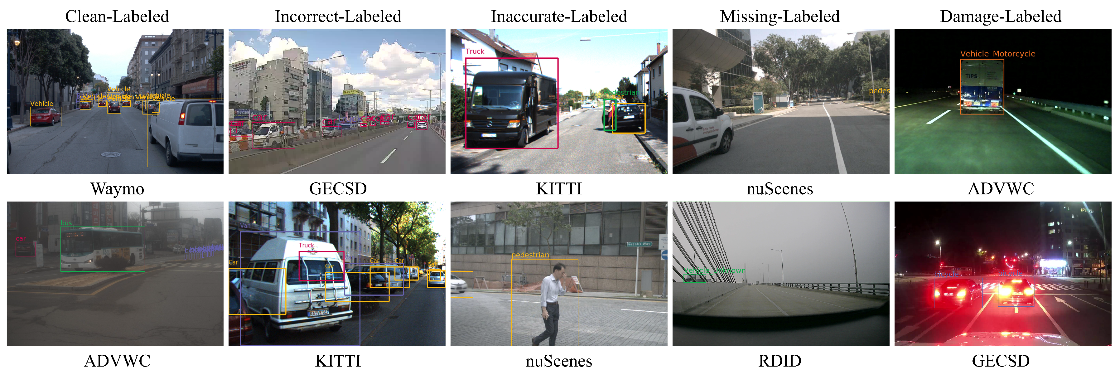
• It automatically finds incorrect, inaccurate, missed, and damaged labels generated during the human annotation process.
• The training efficiency is increased by lowering the priority of duplicate or complex data and excluding it from the training dataset.
• Quality assurance, previously performed by humans on a small number of random pieces of data, can be automated on the entire dataset, saving time and money.
• It is easy to select data that need to be modified and reorganized into a high-quality dataset.

This study proved that not only a large amount of data but also high-quality data are vital for model learning. Data quality was automatically guaranteed by filtering the abnormal data and mitigating the imbalanced data. The model was trained using the dataset built during the noisy label deletion process, and noisy labels were distinguished using the prediction results. The data used for the training were obtained by gathering opinions from multiple models. In a previous study, several models were used [32]. However, the methods used to determine the data that should not be used differ. A trustworthy dataset [32] used single scores, such as F1 and accuracy. However, the proposed study quantified and utilized indicators defined in the standard. It is important to note that incorrect data may still be used during the initial submodel training, which makes the LScores calculated from the prediction results only partially reliable. The LScore calculation includes the confidence score and IoU value. If the overlap between the GT data and prediction bounding box is small, the LScore becomes negligible. This approach is particularly sensitive to small objects, ensuring that they are properly accounted for during the training. This issue can be addressed by adding a process that uses a high-quality dataset, initially selected by an inspector like that in [57]. Additionally, a data and performance verification process needs to be added after the model training steps in the deleting and whitening phases. This will allow for monitoring changes in model performance and verifying data quality. Repeatedly training the model to delete noisy label or whiten the data distribution can lead to overfitting. To address this, it is necessary to add modules that regularize the input data during training or implement early-stopping mechanisms by monitoring performance metrics.

This study will be extended by evaluating different detection models, including diverse architectures such as YOLO and DETR, to examine how model architecture influences noisy label identification. Although the current LScore framework was validated using models of the same type (Faster R-CNN), its application across different detection paradigms presents challenges, such as aligning training configurations, confidence scores, and post-processing schemes. Addressing these challenges is a part of our future work, which includes comparing recent model-based NLL techniques to highlight the advantages of our data-centric approach. However, our approach differs from recent NLL methods [23,24,25] that focus on robust training under label noise conditions. Because our method operates as a preprocessing framework for data quality enhancement, direct experimental comparison is nontrivial. We plan to explore indirect benchmarking by applying our cleaned datasets to NLL pipelines in order to assess their combined effectiveness.

The diversity scores were calculated using a uniform distribution as the ideal value for data distribution whitening. A previous study [46] improved the quality of a dataset by defining its class density and analyzing its correlation with the accuracy of each class. Compared to our study, Sutdy [46] is similar in that it confirms the diversity of the classes. Similarities with the learning data were also measured. Through dynamic data reduction using a binary search technique, only the data necessary for learning were retained and the performance change was confirmed. However, our study confirmed the class and object size distributions. There was also a significant difference in the calculated z-scores for the standard deviation. Through this study, the z-score could identify rare objects that were continuously included in the learning process. Conversely, duplicates or too many subjects were excluded from the study. However, 2D object detection data, particularly autonomous driving data, have been developed for specific purposes. Because we collected data from roads, vehicle objects accounted for more than half of all the objects. However, because the distribution of the actual environment was not considered in the diversity score calculation, it was necessary to follow a natural distribution.

This study aimed to automatically perform quality assurance by performing pruning on a dataset constructed by deleting noisy labels and whitening the data distribution. Cross validation of multiple models was performed to clean the dataset and ensure reliability of the purification criteria. Abnormal data that interfered with learning were automatically classified. The datasets were refined to reduce the data count and hardware overhead. However, the recognition performance of the trained model either improved or remained unchanged. Recently, there have been studies focused on mitigating the impact of noisy labels [58]. A comparative study is needed to determine which is more effective: reducing noisy labels through model-centric approaches or using noise-free datasets via data-centric methods like this study.

7. Conclusions

The study proposed a fully automated framework for validating publicly available datasets before their use, using an AI model for the deletion of noisy labels and data distribution whitening. The framework was tested using six datasets published in South Korea and other countries. Data that are erroneous or harmful to the learning process are automatically filtered and excluded, while the rare classes and objects necessary for data learning are retained through the data-distribution whitening process. Duplicate data are then filtered. The combination of deleting noisy labels and whitening the data distribution is known as data pruning. Redundant or obstructive data are excluded, while only effective data are retained. This process reduces the total amount of data required for learning without significantly changing performance. The study adheres to the ISO/ICE 25012 data quality model standard and the “Data Quality Management Guidelines for AI Learning” of the Korea Ministry of Science and ICT and the Korea Intelligence Information Society Promotion Agency. The model’s accuracy, precision, consistency, and diversity were used as quality evaluation indicators. The proposed framework is versatile and can be applied not only to 2D object detection datasets but also to 3D object detection data and image semantic segmentation datasets.

References

1. Ma, Y.; Wang, Z.; Yang, H.; Yang, L. AI applications in the dev. of autonomous vehicles: A survey. IEEE/CAA J. Autom. Sinica 2020, 7, 315–329. [Google Scholar] [CrossRef]
2. Cunneen, M.; Mullins, M.; Murphy, F. Autonomous vehicles and embedded AI: The challenges of framing machine driving decisions. Appl. Artif. Intell. 2019, 33, 706–731. [Google Scholar] [CrossRef]
3. Howard, J. AI: Implications for the future of work. Am. J. Ind. Med. 2019, 62, 917–926. [Google Scholar] [CrossRef] [PubMed]
4. Roh, Y.; Heo, G.; Whang, S.E. A survey on data collection for ML: A big data-AI integration perspective. IEEE Trans. Knowl. Data Eng. 2019, 33, 1328–1347. [Google Scholar] [CrossRef]
5. Mahmood, R.; Lucas, J.; Acuna, D.; Li, D.; Philion, J.; Alvarez, J.M.; Yu, Z.; Fidler, S.; Law, M.T. How much more data do I need? Estimating requirements for downstream tasks. In Proceedings of the IEEE/CVF Conference on Computer Vision and Pattern Recognitio (CVPR), New Orleans, LA, USA, 18–24 June 2022; pp. 275–284. [Google Scholar]
6. Whang, S.E.; Roh, Y.; Song, H.; Lee, J.G. Data collection and quality challenges in deep learning: A data-centric AI perspective. VLDB J. 2023, 32, 791–813. [Google Scholar] [CrossRef]
7. ISO/IEC 25012:2008; Systems and Software Engineering—Systems and Software Quality Requirements and Evaluation (SQuaRE)—Data Quality with Guidance for Use. International Organization for Standardization: Geneva, Switzerland, 2008.
8. Ministry of Science and ICT of Korea, NIA of Korea. Data Quality Management Guidelines and Construction Guidelines for AI Learning 3—Quality Management Guideline. 2023. Available online: https://aihub.or.kr/aihubnews/qlityguidance/view.do?pageIndex=1&nttSn=10125&currMenu=135&topMenu=103&searchCondition=&searchKeyword= (accessed on 26 October 2024).
9. Gualo, F.; Rodríguez, M.; Verdugo, J.; Caballero, I.; Piattini, M. Data quality certification using ISO/IEC 25012: Industrial experiences. J. Syst. Softw. 2021, 176, 110938. [Google Scholar] [CrossRef]
10. Lytvyn, V.; Vysotska, V.; Demchuk, A.; Bublyk, M.; Demkiv, L.; Shpak, Y. Method of ontology quality assessment for knowledge base in intellectual systems based on ISO/IEC 25012. In Proceedings of the IEEE 15th International Conference on Computer Sciences and Information Technologies (CSIT), Zbarazh, Ukraine, 23–26 September 2020; IEEE: Piscataway, NJ, USA, 2020; Volume 1, pp. 109–113. [Google Scholar]
11. Guerra-García, C.; Nikiforova, A.; Jiménez, S.; Perez-Gonzalez, H.G.; Ramírez-Torres, M.; Ontañon-García, L. ISO/IEC 25012-based methodology for managing data quality requirements in the development of information systems: Towards Data Quality by Design. Data Knowl. Eng. 2023, 145, 102152. [Google Scholar] [CrossRef]
12. Liu, L.; Ouyang, W.; Wang, X.; Fieguth, P.; Chen, J.; Liu, X.; Pietikäinen, M. Deep learning for generic object detection: A survey. Int. J. Comput. Vis. 2020, 128, 261–318. [Google Scholar] [CrossRef]
13. Zaidi, S.S.A.; Ansari, M.S.; Aslam, A.; Kanwal, N.; Asghar, M.; Lee, B. A survey of modern deep learning based object detection models. Digit. Signal Process. 2022, 126, 103514. [Google Scholar] [CrossRef]
14. Li, J.; Socher, R.; Hoi, S.C. DivideMix: Learning with noisy labels as semi-supervised learning. arXiv 2020, arXiv:2002.07394. [Google Scholar]
15. Mnih, V.; Hinton, G.E. Learning to label aerial images from noisy data. In Proceedings of the 29th International Conference on Machine Learning (ICML-12), Edinburgh, Scotland, 26 June–1 July 2012; pp. 567–574. [Google Scholar]
16. Kim, Y.; Kim, J.M.; Akata, Z.; Lee, J. Large loss matters in weakly supervised multi-label classification. In Proceedings of the IEEE/CVF Conference on Computer Vision and Pattern Recognition (CVPR), New Orleans, LA, USA, 18–24 June 2022; pp. 14156–14165. [Google Scholar]
17. Ghosh, A.; Manwani, N.; Sastry, P. On the robustness of decision tree learning under label noise. In Proceedings of the Pacific-Asia Conference on Knowledge Discovery and Data Mining (PAKDD), Jeju, Republic of Korea, 23–26 May 2017; pp. 685–697. [Google Scholar]
18. Zha, D.; Bhat, Z.P.; Lai, K.H.; Yang, F.; Jiang, Z.; Zhong, S.; Hu, X. Data-centric Artificial Intelligence: A Survey. arXiv 2023, arXiv:2303.10158. [Google Scholar] [CrossRef]
19. Zhou, X.; Chai, C.; Li, G.; Sun, J. Database meets AI: A survey. IEEE Trans. Knowl. Data Eng. 2020, 34, 1096–1116. [Google Scholar] [CrossRef]
20. Geiger, A.; Lenz, P.; Stiller, C.; Urtasun, R. Vision meets robotics: The KITTI dataset. Int. J. Robot. Res. 2013, 32, 1231–1237. [Google Scholar] [CrossRef]
21. Sun, P.; Kretzschmar, H.; Dotiwalla, X.; Chouard, A.; Patnaik, V.; Tsui, P.; Guo, J.; Zhou, Y.; Chai, Y.; Caine, B. Scalability in perception for autonomous driving: Waymo open dataset. In Proceedings of the IEEE/CVF Conference on Computer Vision and Pattern Recognition (CVPR), Seattle, WA, USA, 14–19 June 2020; pp. 2446–2454. [Google Scholar]
22. Caesar, H.; Bankiti, V.; Lang, A.H.; Vora, S.; Liong, V.E.; Xu, Q.; Krishnan, A.; Pan, Y.; Baldan, G.; Beijbom, O. nuScenes: A multimodal dataset for autonomous driving. In Proceedings of the IEEE/CVF Conference on Computer Vision and Pattern Recognition (CVPR), Seattle, WA, USA, 14–19 June 2020; pp. 11621–11631. [Google Scholar]
23. Wang, W.; Li, Y.; Li, A.; Zhang, J.; Ma, W.; Liu, Y. An Empirical Study on Noisy Label Learning for Program Understanding. In Proceedings of the IEEE/ACM International Conference on Software Engineering (ICSE), Lisbon, Portugal, 14–20 April 2024; pp. 1–12. [Google Scholar]
24. Deng, L.; Yang, B.; Kang, Z.; Wu, J.; Li, S.; Xiang, Y. Separating hard clean samples from noisy samples with samples’ learning risk for DNN when learning with noisy labels. Complex Intell. Syst. 2024, 10, 4033–4054. [Google Scholar] [CrossRef]
25. Zhang, J.; Song, B.; Wang, H.; Han, B.; Liu, T.; Liu, L.; Sugiyama, M. Badlabel: A robust perspective on evaluating and enhancing label-noise learning. IEEE Trans. Pattern Anal. Mach. Intell. 2024, 46, 4398–4409. [Google Scholar] [CrossRef]
26. Natarajan, N.; Dhillon, I.S.; Ravikumar, P.K.; Tewari, A. Learning with noisy labels. Adv. Neural Inf. Process. Syst. 2013, 26, 1–9. [Google Scholar]
27. Song, H.; Kim, M.; Park, D.; Shin, Y.; Lee, J.G. Learning from noisy labels with DNNs: A survey. IEEE Trans. Neural Netw. Learn. Syst. 2022, 34, 1–19. [Google Scholar]
28. He, H.; Garcia, E.A. Learning from imbalanced data. IEEE Trans. Knowl. Data Eng. 2009, 21, 1263–1284. [Google Scholar]
29. Liu, D.; Tsang, I.W.; Yang, G. A convergence path to deep learning on noisy labels. IEEE Trans. Neural Netw. Learn. Syst. 2022. [Google Scholar] [CrossRef]
30. Oleghe, O. A predictive noise correction methodology for manufacturing process datasets. J. Big Data 2020, 7, 1–27. [Google Scholar] [CrossRef]
31. Xiong, H.; Pandey, G.; Steinbach, M.; Kumar, V. Enhancing data analysis with noise removal. IEEE Trans. Knowl. Data Eng. 2006, 18, 304–319. [Google Scholar] [CrossRef]
32. Sun, Y.; Gu, Z. Using computer vision to recognize construction material: A Trustworthy Dataset Perspective. Resour. Conserv. Recycl. 2022, 183, 106362. [Google Scholar] [CrossRef]
33. Zhang, J.; Wu, M.; Zhou, C.; Sheng, V.S. Active crowdsourcing for multilabel annotation. IEEE Trans. Neural Netw. Learn. Syst. 2022, 35, 3549–3559. [Google Scholar] [CrossRef] [PubMed]
34. Zhang, J.; Sheng, V.S.; Li, T.; Wu, X. Improving crowdsourced label quality using noise correction. IEEE Trans. Neural Netw. Learn. Syst. 2017, 29, 1675–1688. [Google Scholar] [CrossRef]
35. Zhang, C.; Zhang, H.; Xie, W.; Liu, N.; Li, Q.; Jiang, D.; Lin, P.; Wu, K.; Chen, L. Cleaning uncertain data with crowdsourcing-a general model with diverse accuracy rates. IEEE Trans. Knowl. Data Eng. 2020, 34, 3629–3642. [Google Scholar] [CrossRef]
36. Wu, X.; Jiang, L.; Zhang, W.; Li, C. Three-way decision-based noise correction for crowdsourcing. Int. J. Approx. Reason. 2023, 160, 108973. [Google Scholar] [CrossRef]
37. Xu, N.; Li, J.Y.; Liu, Y.P.; Geng, X. Trusted-data-guided label enhancement on noisy labels. IEEE Trans. Neural Netw. Learn. Syst. 2022, 34, 9940–9951. [Google Scholar] [CrossRef]
38. Contardo, G.; Denoyer, L.; Artières, T. A meta-learning approach to one-step active learning. arXiv 2017, arXiv:1706.08334. [Google Scholar]
39. Bernhardt, M.; Castro, D.C.; Tanno, R.; Schwaighofer, A.; Tezcan, K.C.; Monteiro, M.; Bannur, S.; Lungren, M.P.; Nori, A.; Glocker, B. Active label cleaning for improved dataset quality under resource constraints. Nat. Commun. 2022, 13, 1161. [Google Scholar] [CrossRef]
40. Bachman, P.; Sordoni, A.; Trischler, A. Learning algorithms for active learning. In Proceedings of the International Conference on Machine Learning, Sydney, Australia, 6–11 August 2017; PMLR: Breckenridge, CO, USA, 2017; pp. 301–310. [Google Scholar]
41. Sener, O.; Savarese, S. Active learning for convolutional neural networks: A core-set approach. arXiv 2017, arXiv:1708.00489. [Google Scholar]
42. Takezoe, R.; Liu, X.; Mao, S.; Chen, M.T.; Feng, Z.; Zhang, S.; Wang, X. Deep active learning for computer vision: Past and future. APSIPA Trans. Signal Inf. Process. 2023, 12, 1–18. [Google Scholar] [CrossRef]
43. Khosla, A.; Zhou, T.; Malisiewicz, T.; Efros, A.A.; Torralba, A. Undoing the damage of dataset bias. In Proceedings of the European Conference on Computer Vision (ECCV), Florence, Italy, 7–13 October 2012; Springer: Berlin/Heidelberg, Germany, 2012; pp. 158–171. [Google Scholar]
44. Li, Y.; Vasconcelos, N. REPAIR: Removing representation bias by dataset resampling. In Proceedings of the IEEE/CVF Conference on Computer Vision and Pattern Recognition (CVPR), Long Beach, CA, USA, 15–20 June 2019; pp. 9572–9581. [Google Scholar]
45. Chen, H.; Chen, J.; Ding, J. Data evaluation and enhancement for quality improvement of ML. IEEE Trans. Reliab. 2021, 70, 831–847. [Google Scholar] [CrossRef]
46. Byerly, A.; Kalganova, T. Class density and dataset quality in high-dimensional, unstructured data. arXiv 2022, arXiv:2202.03856. [Google Scholar]
47. Chen, K.; Chen, H.; Conway, N.; Hellerstein, J.M.; Parikh, T.S. Usher: Improving data quality with dynamic forms. IEEE Trans. Knowl. Data Eng. 2011, 23, 1138–1153. [Google Scholar] [CrossRef]
48. Pičuljan, N.; Car, Ž. Machine learning-based label quality assurance for object detection projects in requirements engineering. Appl. Sci. 2023, 13, 6234. [Google Scholar] [CrossRef]
49. Li, C.; Mao, Z.; Jia, M. A real-valued label noise cleaning method based on ensemble iterative filtering with noise score. Int. J. Mach. Learn. Cybern. 2024, 15, 1–26. [Google Scholar] [CrossRef]
50. Fang, M.; Zhou, T.; Yin, J.; Wang, Y.; Tao, D. Data subset selection with imperfect multiple labels. IEEE Trans. Neural Netw. Learn. Syst. 2018, 30, 2212–2221. [Google Scholar] [CrossRef]
51. Wu, Y.; Kirillov, A.; Massa, F.; Lo, W.Y.; Girshick, R. “Detectron2”. 2019. Available online: https://github.com/facebookresearch/detectron2 (accessed on 26 October 2024).
52. Ren, S.; He, K.; Girshick, R.; Sun, J. Faster R-CNN: Towards real-time object detection with region proposal networks. Adv. Neural Inf. Process. Syst. 2015, 28, 1–9. [Google Scholar] [CrossRef]
53. Girshick, R. Fast R-CNN. In Proceedings of the IEEE International Conference on Computer Vision (ICCV), Santiago, Chile, 7–13 December 2015; pp. 1440–1448. [Google Scholar]
54. Korea Automobile Research Institute. Road Driving Image Data. 2020. Available online: https://www.aihub.or.kr/aihubdata/data/view.do?currMenu=115&topMenu=100&aihubDataSe=data&dataSetSn=180 (accessed on 26 October 2024).
55. Korea National Information Society Agency. Autonomous Driving Data in Various Weather Conditions Dataset. 2021. Available online: https://www.aihub.or.kr/aihubdata/data/view.do?currMenu=115&topMenu=100&aihubDataSe=data&dataSetSn=630 (accessed on 26 October 2024).
56. Korea Transportation Safety Authority. Generic and Edge Case Scenario Data. 2021. Available online: https://avds.kotsa.or.kr/open/normal/Open_Normal_List.do?bbs_seq=3010 (accessed on 4 November 2024).
57. Chu, Z.; Zhang, R.; Yu, T.; Jain, R.; Morariu, V.; Gu, J.; Nenkova, A. Self-Cleaning: Improving a Named Entity Recognizer Trained on Noisy Data with a Few Clean Instances. In Proceedings of the Findings of the Association for Computational Linguistics (NAACL2024), Mexico City, Mexico, 16–21 June 2024; pp. 196–210. [Google Scholar]
58. Chen, M.; Zhao, Y.; He, B.; Han, Z.; Huang, J.; Wu, B.; Yao, J. Learning with Noisy Labels Over Imbalanced Subpopulations. IEEE Trans. Neural Netw. Learn. Syst. 2024, 36, 6544–6555. [Google Scholar] [CrossRef]
Figure 1. The overall framework of this study. We have noisy data or a dataset with an imbalanced distribution. Shown is the proposed automated two-step process for refining the 2D object detection dataset.
Electronics 14 01882 g001
Figure 2. Examples of abnormal data include misclassification, misaligned or missing bounding boxes, and corrupted label files. Each box in the image represents a detected object corresponding to a class in the dataset. Since the image is based on the original labeling data, the class labels appear overlapped in densely populated areas.
Electronics 14 01882 g002
Figure 3. Flowchart of the process of deleting noisy labels. This process operates in three steps: model training, labeling score ensemble, and deletion.
Electronics 14 01882 g003
Figure 4. Flowchart of the data distribution whitening process. This process involves three steps: calculating the diversity scores, whitening the data, and training the model.
Electronics 14 01882 g004
Figure 5. Illustration of why LScores should be combined with whitening scores. (a) shows data with rare but noisy labels and (b) shows common objects with clean labels.Red text indicates negative aspects, while blue text indicates positive ones.
Electronics 14 01882 g005
Figure 6. Results of noisy label deletion on the KITTI dataset. (ac) show examples of filtered incorrect, inaccurate, and missing labels, respectively. (a) Filtered incorrect label. (b) Filtered inaccurate label. (c) Filtered missing label. Each box represents a labeled object in the dataset. Purple indicates the vehicle class, orange indicates pedestrian, yellow represents cyclist, and light blue corresponds to the don’t care class. Since the image is based on the original labeling data, text labels may appear overlapped in densely populated areas. The red- and green-bordered images on the right show zoomed-in views of the corresponding regions marked on the left.
Electronics 14 01882 g006
Figure 7. Results of noisy label deletion on the nuScenes dataset. (ac) show examples of incorrect, missing, and inaccurate labels. (a) Filtered incorrect label. (b) Filtered missing label. (c) Filtered inaccurate label. The pink boxes represent the truck class, while the purple boxes indicate the car class. Since the image is based on the original labeling data, text labels may appear overlapped in densely populated areas. The red-bordered image on the right is a zoomed-in view of the red-bordered region on the left.
Electronics 14 01882 g007
Figure 8. Results of noisy label deletion on the ADVWC dataset. (ac) show examples of missing and incorrect labels under severe weather conditions. (a) Filtered missing label. (b) Filtered missing label. (c) Filtered incorrect label. The pink boxes represent the car class, the light green boxes indicate central reservation, the orange boxes correspond to bollard, and the purple boxes denote instruction line. Due to the use of original annotation data, overlapping class labels can be observed in regions with high object density. The red- and green-bordered images on the right show zoomed-in views of the corresponding regions marked on the left.
Electronics 14 01882 g008
Figure 9. Results of noisy label deletion on the GECSD dataset. (ac) show examples of damaged or missing labels caused by class reversal and annotation errors. (a) Filtered damaged label. (b) Filtered damaged label. (c) Filtered missing label. Yellow, light green, light blue, pink, lavender, and purple boxes represent the bus, truck, traffic sign, car, person, and bicycle classes, respectively. Due to the use of original labeling data, text annotations may overlap in regions with high object density. The red-, blue-, and green-bordered images on the right show zoomed-in views of the corresponding regions marked on the left.
Electronics 14 01882 g009
Figure 10. Effects of data distribution whitening on the KITTI dataset. (a) shows the change in class distribution, and (b) shows the bounding box size distribution before and after whitening. The colors are used to distinguish different classes. Some objects appear as dots because their distribution is too small, making the circles look like points.
Electronics 14 01882 g010
Figure 11. Example of Waymo data excluded from training because of a low whitening score. The purple boxes represent the Vehicle class. Since the image is based on the original labeling data, the Vehicle texts appear overlapped in densely populated areas. The Waymo dataset had the highest distribution of car objects, and the data for these objects were reduced.
Electronics 14 01882 g011
Figure 12. Low-priority nuScenes data filtered by whitening score, including small or inaccurately labeled objects such as pedestrians, cars, and barriers. The pink, purple, light green, and light blue boxes indicate trucks, vehicles, pedestrians, and barriers, respectively. Since the image is based on the original labeling data, the class labels appear overlapped in densely populated areas.
Electronics 14 01882 g012
Figure 13. Changes in class and bounding box size distributions in the nuScenes dataset after whitening. (a) shows reduced objects by class, and (b) shows size-based reduction, mainly affecting small objects. The colors are used to distinguish different classes. Some objects appear as dots because their distribution is too small, making the circles look like points.
Electronics 14 01882 g013