Enhancing Machine Learning Techniques in VSLAM for Robust Autonomous Unmanned Aerial Vehicle Navigation

Abstract

This study introduces a visual SLAM real-time system designed for small indoor environments. The system demonstrates resilience against significant motion clutter and supports wide-baseline loop closing, re-localization, and automatic initialization. Leveraging state-of-the-art algorithms, the approach presented in this article utilizes adapted Oriented FAST and Rotated BRIEF features for tracking, mapping, re-localization, and loop closing. In addition, the research uses an adaptive threshold to find putative feature matches that provide efficient map initialization and accurate tracking. The assignment is to process visual information from the camera of a DJI Tello drone for the construction of an indoor map and the estimation of the trajectory of the camera. In a ’survival of the fittest’ style, the algorithms selectively pick adaptive points and keyframes for reconstruction. This leads to robustness and a concise traceable map that develops as scene content emerges, making lifelong operation possible. The results give an improvement in the RMSE for the adaptive ORB algorithm and the adaptive threshold (3.280). However, the standard ORB algorithm failed to achieve the mapping process.

1. Introduction

Unmanned Autonomous Vehicles need to sense, analyze, and understand their environment to carry out tasks like following a path, planning movements, avoiding obstacles, and identifying targets. Global Navigation Satellite Systems (GNSSs) provide reliable real-time positioning and environmental information for autonomous platforms like autonomous navigation systems and Autonomous Vehicles (AVs). In dense and cluttered environments, Unmanned Aerial Vehicles (UAVs) can experience challenges with GNSS signals due to issues like signal fading, multi-path interference, jamming, and spoofing, which can lead to signal degradation or loss. As a result, a GNSS becomes less dependable for UAV operations at low altitudes in areas with heavy obstructions, such as urban landscapes, forests, or mountainous regions [1,2]. Researchers have recently developed various localization methods tailored for UAVs, such as vision-based and LIDAR-based systems. However, integrating multiple sensors for robotic localization can be expensive and may increase the system’s weight and energy consumption. The challenges mentioned above have impeded the widespread implementation of several robot localization algorithms [3].

Visual localization, a computer vision-based technology, has emerged as an attractive alternative. Visual localization operates by acquiring environmental images through a camera, which are then processed to estimate the system’s pose—its position and orientation—enabling the mapping of previously unknown environments. One benefit of this technology is that the cost of the camera is relatively low, and the camera can capture a wide variety of environmental information, for example, visual information such as texture and color [1]. However, visual localization requires high computational power; images are memory-intensive, and visual localization software is comparatively complex to develop. In addition, the visual system is also influenced by light conditions, and it may not perform optimally under conditions where lighting is inadequate.

Visual Simultaneous Localization and Mapping helps minimize drift in state estimation by revisiting previously mapped areas, producing a globally consistent representation of the environment [3]. There are many solutions and methods to visual SLAM problems. The main approaches are feature-based methods [4] and the direct methods [5]. Keypoints are used in feature-based techniques.

These techniques involve saving critical points to keyframes or local submaps, followed by the use of a graph optimization technique. Direct SLAM techniques, on the other hand, save every pixel of an image on a local map and estimate measurement errors using photometric losses. Contemporary SLAM techniques vary greatly and are typically fairly modular. Furthermore, SLAM with dynamic objects is solved using several cutting-edge techniques. In recent years, SLAM methods using sensors other than RGB cameras have been created. As an illustration, consider stereo and RGB-D (depth) cameras [6], IMU measurements [7], and LIDAR point cloud transformations [8]. A consistent solution to the SLAM problem is obtained by combining various environmental data. For this reason, the methodologies need to be applied and assessed on datasets that have a variety of sensors. Open VSLAM, Open VINS, VINS-Mono, MapLab, LDSO, VINS-Fusion, Kimera, ORB-SLAM 2/3, DRE, and Basalt are feature-based solutions for visual SLAM methods. As we can see later, the main goal of this study is to enhance the ORB-SLAM’s detect and extract feature, which is considered the main block in the visual SLAM.

The paper is organized as follows: Section 2 presents the most related methods of the research topic for localization and mapping. Section 3 explains the experimental setup and adjusts the adaptive parameters and the threshold. In addition, it provides a specific database description. It presents the steps of map initialization (detect and extract features by using the adaptive parameters, describe feature matching, and present the initialization of the place recognition database by using the adaptive threshold). After map initialization, the local tracking step is performed using every keyframe. Next, the loop closure detection takes the current keyframe processed by the local mapping process and tries to detect and close the loop. At the end of this section, there is a comparison with the actual camera trajectory to evaluate the accuracy. Section 4 analyses the results and compares them with the old algorithms. The last section concludes the results, and further research steps are presented into how VSLAM can be more effectively applied in autonomous vehicle navigation.

2. Related Work

Several sensors provide data that are utilized for localization and mapping. Examples include stereo, global, rolling shutter, depth, and 3D LIDARs, as well as cameras with global and 2D shutters. Although highly precise, LIDARs are also incredibly expensive. In addition, to measure distance, they must emit light signals. LIDARs are active sensors as a result. Rolling shutter cameras are among the best sensors available for robotics. They are inexpensive, passive, and dense. They simply need to take in information about their surroundings; they do not need to emit light. Although they cost more, global shutter cameras may be more practical. Furthermore, stereo and depth cameras are suitable and popular, similar to the D435 model. For this issue, R. Singh and K. S. Nagla thoroughly assessed contemporary sensors in [9]. While they can all be utilized in SLAM pipelines, each has unique qualities crucial for resolving SLAM issue (see Equation (1)).

The last part of (1) is formulated as maximization of conditional probability $\left(P\right)$ of the robot’s states $\left(X\right)$ and landmarks $\left(M\right)$, given sensor measurements $\left(Z\right)$ and information matrices $(\Omega )$, which are equivalent to minimization of the minus logarithm of P in the case of Gaussian structure of the sensors’ noises. It is comparable to solving a non-linear least-squares problem or kernel-based $\left(\rho \right)$ minimization for robustness in the case of measurement outliers.

$$\begin{array}{cc}\hfill \widehat{X},\widehat{M}& =arg\underset{X,M}{max}P(X,M\mid Z)\hfill \\ \hfill & \simeq arg\underset{X,M}{min}\left[-logP(X,M\mid Z)\right]\hfill \\ \hfill & \equiv arg\underset{X,M}{min}\sum _{i,j}\rho (X_{ij},M_{ij},{\Omega }_{ij})\hfill \end{array}$$

(1)

It is important to note that the primary distinction between visual/visual–inertial odometry and SLAM is that the latter modifies the map $\left(M\right)$ in addition to updating the robot’s states $\left(X\right)$. Cadena et al., for instance, provided an excellent summary of contemporary SLAM technology and the difficulties that SLAM techniques face [10]. Another review [11] claims that SLAM is entering the spatial artificial intelligence era. This implies that the solution is to employ more deep learning algorithms.

The history of visual SLAM is where feature-based SLAM, also known as sparse visual SLAM, started. A technique described by Davison et al. [12] was one of the first to address simultaneous localization and mapping successfully. The algorithm is known as MonoSLAM. The camera position was determined from supplied photos. The utilization of probabilistic filter-based techniques allowed the authors to solve the SfM (Structure from Motion) problem more quickly. The algorithm can obtain the camera trajectory and landmark point positions in real time.

Several drawbacks exist with the MonoSLAM technique. The filtering approach’s poor scaling is the first issue. The requirement to update the trajectory and feature positions sequentially in the same thread is the MonoSLAM algorithm’s other drawback. The Parallel Tracking and Mapping (PTAM) algorithm enables real-time performance on an approach that does complete batch updates, proposed by Klein et al. [13], as a solution to this issue. Furthermore, it was demonstrated by the authors of the paper [14] that bundle adjustment-based solutions [13] outperform filter-based ones.

The ORB-SLAM algorithm, which was covered in the article [4], made a significant addition to the field of problem-solving for visual SLAM. The authors of the research [15] included the essential components of visual SLAM approaches, including the g2o [16] optimizer. The ORB algorithm for fast keypoint detection and description and also the Bags of Binary Words for visual terrain recognition system were presented. Gálvez-López et al. in [17] also merged all prior methods into a single framework. Because scale drifts affect the ORB-SLAM approach, another information source, like an IMU sensor, is frequently employed to indicate the geometric scale. Kurdel et al. in [18] focused on the increasing demand for UAV safety and security, highlighting the need for national legislation in Slovakia by European progress in 2018–2019. Safe UAV flights were emphasized, with an emphasis on flight over mountainous terrain. The research is to model and analyze UAV vertical flight to clear mountain obstacles and propose methods of safe flight maneuvering while complying with Slovak legislative standards. Key findings are the dependence of flight accuracy on estimate approximations, the influence of ambient air temperature on engine thrust and aerodynamic properties, and the necessity for correct flight programming considering UAV system response times. The study aims to optimize flight paths and maintain high safety levels.

Pecho et al. in [19] explored the low utilization of UAVs in agriculture, film, photogrammetry, and research with an argument that formational flying will enhance their use considerably. The paper covers UAV formation flight at its present level, coordination structures, and future use. In their technology analysis on how to have many UAVs forming specialized hardware and structure, high-level mission planning and software for swarms are suggested to be utilized. UAV formations can be created in various shapes for delivery, search and rescue, and medical transport operations. The research utilized virtual simulations to optimize swarm flight, and the most efficient one was arrow formation due to its low energy consumption. Other optimizations include elevating rear UAVs to reduce power consumption. The method replaces accurate experimental tests with a more affordable and time-efficient alternative. The outcomes can be applied in various vocational applications, including fire searching, photogrammetry, and “Smart Hangar” systems, demonstrating the applications of UAV swarms for various uses. The paper [20] presented the VINS algorithm, which combines sequential pictures and IMU data to compute odometry using the Kalman filter. The authors relocated the camera using global optimization as an improvement procedure of research [21]. In [22], one may think of ORB-SLAM2’s development as SOFT-SLAM. The algorithms presented there made the following modifications:

• By using SOFT visual odometry, which achieves an inaccuracy of roughly 0.8% relative to the distance traveled, localization can be accomplished without the more computationally demanding bundle correction.
• Since the streams in charge of mapping and odometry are independent of one another, the thread in charge of mapping does not impede the visual odometry stream, which results in a more consistent processing time for incoming frames. Furthermore, the algorithm is deterministic, meaning it consistently yields the same output for the same input, in contrast to ORB-SLAM2.
• Like ORB-SLAM2, SOFT keypoints are employed for loop closure, which results in a highly dependable, straightforward, and efficient system that achieves subpixel precision, although SOFT critical points are rational invariant. The authors demonstrated on publicly available datasets that loop closure happens frequently enough in practice. This disadvantage has minimal bearing on the outcome.

ORB-SLAM2-CNN [23] is available, which enhances the ORB-SLAM2 framework with semantic data obtained from the neural network. Dense or direct approaches do not use algorithmic characteristics in their work, in contrast to methods for solving the visual SLAM problem based on keypoints. For every pair of photos, they employ photometric error minimization to determine the orientation and position of the camera in three dimensions. DTAM [24] was the first study to propose the use of direct methods.

The DTAM algorithm produced a dense 3D map for every pixel in every image. The following approach is called KineticFusion [25], and it creates a dense 3D map by using a depth camera. The authors describe each pixel using the truncated signed distance function (TSDF), and each depth image is mapped to a map using the Iterative Closest Point technique (ICP). The ElasticFusion [26] algorithm marked the next significant advancement in the development of direct methods. This algorithm directly represents the surfaces of RGB-D cameras.

This approach uses a non-rigid deformation model for data fusion. Additionally, it does not optimize the camera position graph globally, and the majority of the steps are executed on a graphics processing unit (GPU).

Two more teams were working on semi-dense visual odometry (SVO) at the same time as KineticFusion and ElasticFusion [27,28]. This method can be implemented in real-time on a robot’s embedded system. The SVO algorithm uses only the pixels with a slight gradient, not all in the picture. LSD-SLAM was presented in [5], which is a seminal work in this field. The result of the developed concepts was based on the article [27]. LSD-SLAM employs the metric sim to tackle a problem with an unclear scale (3). It also uses probabilistic inference to ascertain the mistake in creating three-dimensional maps. The three steps of the LSD-SLAM algorithm are as follows:

• After obtaining the image, find the local offset concerning the active keyframe.
• Revise or produce a fresh keyframe. If modified, the stereo depth data are probabilistically combined with the current keyframe. When a new keyframe is created, propagate the old depth map to the new one.
• Applying position graph optimization to update the global map. The $g2o$ library is used for optimization, and the $sim\left(3\right)$ metric is used to look for edges in the graph.

SLAM solutions typically assume that the scene has little to no dynamics or is nearly static. Using RANSAC is the most straightforward method of eliminating outliers [29]. Generally speaking, there will be many dynamic objects in every situation. There are many people, animals, vehicles, walkers, bicycles, and other moving items in indoor and outdoor environments. As a result, feature maps are altered. This is particularly crucial for detecting loop closure.

Furthermore, because most SLAM solutions lack trustworthy qualities, they may produce inconsistent outcomes in the case of a high level of dynamics. Dynamic objects come with several issues. First, the algorithms should detect the dynamic item, and they should not use it for either the mapping or trajectory estimation process. Two potential solutions are removing these items from the picture or replacing them with a background. Multi-view geometry [30], semantic segmentation or detection neural networks [31], scene [32], optical flow, and background or foreground detection [33] are popular tools for that.

Second, a consistent map must be created, dynamic objects included or not. Resolving the issue of insufficient data resulting from the removal of dynamic objects is a crucial component. It may be possible to improve things with more sensors, object completion, reconstruction, and other map generation methods [34,35]. Dynamic SLAM methods are frequently used to model intricate, multi-component systems that operate in non-real time.

3. VSLAM Techniques for UAV Mapping: Difficulties and Experimental Setup

As is widely known, ORB-SLAM algorithms suffer from significant limitations in dynamic environments, primarily due to their reliance on fixed parameters defined a priori. This causes them to perform poorly in changing lighting conditions or low-texture environments, where the number of keypoints detected decreases, negatively impacting the mapping and tracking processes. Classical ORB-SLAM algorithms also require parameter tuning manually, making them inefficient for real-time applications that constantly require adaptation. To solve this challenge, an adaptive method is proposed in which essential values are changed dynamically instead of fixed. By allowing these parameters to be adaptive, the research makes the ORB-SLAM algorithm more efficient and stable than the traditional ORB-SLAM algorithm. For example, when the number of keypoints found in a frame is too low, the system will redo feature matching and data extraction instead of continuing with too little information. This provides a credible map building and path point, resulting in a more solid and dependable SLAM system. This learning process renders the algorithm less sensitive to adverse conditions, such as low-texture scenes, changing lighting, and motion noise. Consequently, our method provides a more robust and efficient SLAM solution, especially for real-world applications, where fixed parameter settings easily result in failure or inaccuracy. This section gives the complete process of the method presented ins the paper, starting from capturing images with a drone camera to generating a map of the path. The experiment will use the ORB-SLAM, which is a feature-based VSLAM algorithm. Figure 1 represents the flowchart of the feature-based VSLAM step by step, starting from preparing the video, converting it to a subset of video frames, adjusting the labels of the dataset, splitting the data to training and testing sets, image processing and filtering, extracting and detecting features, map initialization, local mapping, tracking, and loop closure. VSLAM algorithms are typically categorized into two main components, which consist of front-end and back-end processes:

• Front-end algorithms process sensor data to estimate the camera’s pose and extract 3D map points from the environment.
• Back-end algorithms refine the camera trajectory and map through optimization techniques, ensuring consistency across the entire system.

This experiment aims to enhance the traditional ORB-SLAM, which relies on fixed parameters, by developing a new method that utilizes adaptive parameters. This adaptation allows the algorithm to perform better in dynamic environments, specifically changing lighting conditions.

3.1. Experimental Setup and Environment

The experimental simulations, processing time measurements, and RMSE calculations were performed on the following hardware configuration:

• CPU: Intel® Core™ i7-11800H @ 2.30GHz (8 cores, 16 threads); Intel Corporation, Santa Clara, CA, USA.
• GPU: NVIDIA® GeForce RTX™ 3060 Laptop GPU with 6 GB GDDR6 VRAM; NVIDIA Corporation, Santa Clara, CA, USA.
• RAM: 32 GB DDR4 3200 MHz; Kingston Technology, Fountain Valley, CA, USA.
• Storage: 1 TB NVMe SSD; Samsung Electronics Co., Ltd., Suwon, Republic of Korea.
• System Architecture: 64-bit.
• Operating System: Windows 11 Pro, Version 23H2; Microsoft Corporation, Redmond, WA, USA.

• Software Environment:

• MATLAB: Version R2022a;
• Programming Language: MATLAB, with custom scripts for adaptive parameter tuning, feature extraction, and trajectory evaluation.

3.2. Database Description

Initially, creating the database was the fundamental step for the entire procedure. Utilizing a fixed camera on a DJI Tello drone enabled this approach Figure 2.

The camera records the video, whose frames are acquired and resized according to the camera specifications to provide a resolution of $(640\times 480)$ pixels. This provides a set of images constituting the database for this work, and the number of acquired frames determines the database size. Two consecutive images, $I_t$ and $I_{t+1}$, are chosen from the acquired frames from the camera, and these are then undistorted. Initially, front-end algorithms are used to construct a 3D map of the environment and estimate the camera pose. Back-end algorithms then refine the initial estimates by optimizing the camera trajectory and map points, improving the overall reconstruction process’s accuracy. Figure 3 and Figure 4 show the database experiment and the first frame of it.

3.3. Map Initialization

The feature-based Visual Simultaneous Localization and Mapping (V-SLAM) method initiates by establishing a map of 3D points derived from two video frames. This process involves computing the 3D points and relative camera pose through triangulation, which relies on 2D Oriented FAST and Rotated BRIEF (ORB) feature correspondences [36]. This step is crucial and has a significant impact on the accuracy of the final SLAM result.

3.3.1. Detect and Extract Features

Features represent digital expressions of image data. A practical set of features is essential for optimal performance on the designated task, prompting researchers to invest significant effort in feature extraction. Unlike deep learning approaches, classical computer vision relies on handcrafted features, which are often defined as keypoints and specific, distinctive regions within an image that are used for matching and recognition. Figure 5 shows the corners, edges, and blocks as representative places in the image.

A feature point is typically defined by two elements: the keypoint, representing the position of a salient region in the image, and the descriptor, which captures the local visual characteristics for comparison and matching.

• Keypoint: This denotes the 2D position of a feature within the image. Specific keypoints may also store auxiliary information, such as scale and orientation, to support invariance to viewpoint or image resolution changes.
• Descriptor: A descriptor is a numerical vector characterizing the visual content around a keypoint. It is designed to ensure that similar-looking regions produce descriptors close in vector space, enabling robust feature matching across images.

For real-time feature extraction, the Oriented FAST and Rotated BRIEF (ORB) feature is widely used. It uses a modified version of FAST (Oriented FAST) with the extremely fast binary descriptor BRIEF, significantly accelerating the entire image feature extraction process. To achieve the goal of the research, an updated algorithm to detect and extract the ORB features will first be developed and used. The normal ORB detection feature uses fixed parameters. The algorithm presented here uses adapted parameters, which are adjusted from the program code and will start working until suitable parameters (scaleFactor, numLevels, numPoints) are found for perfect detection. These parameters are as follows:

• scaleFactor: This parameter determines the factor by which the image is resized at each scale level when constructing the image pyramid for feature detection. A smaller scale factor will lead to more levels in the pyramid, resulting in finer-scale features being detected, but it will also increase computation time. Conversely, a larger scale factor will reduce the number of pyramid levels and may miss smaller-scale features but will reduce computation time.
• numLevels: This parameter specifies the number of levels in the image pyramid used for feature detection. Each level represents a scaled version of the original image. More levels allow for the detection of features at different scales but also increase computational complexity. Typically, a higher number of levels leads to more fine-scale features being detected.
• numPoints (or nFeatures): This parameter determines the maximum number of keypoints (feature points) to be detected in the image. The ORB feature detector aims to detect a fixed number of keypoints, and numPoints controls this number.

The core principle behind ORB (Oriented FAST and Rotated BRIEF) feature extraction is that a pixel with a significantly different intensity than its neighboring pixels—either much brighter or darker—will likely be a corner point. The complete ORB extraction process is outlined below and illustrated in Figure 6:

• Select pixel p in the image assuming its brightness as $I_p$.
• Set a threshold T (for example, 20% of $I_p$ “this is a fixed one”).
• Take the pixel p as the center and select the 16 pixels on a circle with a radius of 3.
• If there are consecutive N points on the selected circle whose brightness is greater than $I_p+T$ or less than $I_p-T$, then the central pixel p can be considered a feature point. The value of N is usually 12, 11, or 9.
• Iterate through the above four steps on each pixel.

A trick is used to reject most non-corner points by first examining the pixels at positions 1, 9, 5, and 13. At least N of these pixels must have a brightness greater than $(I_p+T)$ or less than $(I_p-T)$ for the point to be considered a corner. Oriented Feature from Accelerated Segment Test (oFAST) is used to detect feature points in an image and compute their orientations to achieve rotation invariance. The process of oFAST is illustrated in Figure 7. The steps involved are the following:

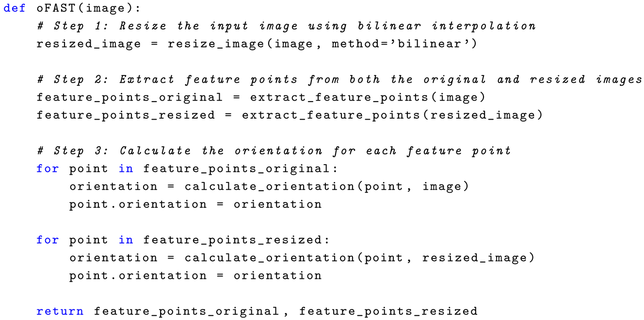
• Begin by resizing the input image using bilinear interpolation.
• Next, extract feature points from both the original and the resized images.
• Finally, calculate the orientation for each feature point.

To compute the orientations, a circular patch is defined around each feature point. The moments of this patch, denoted as $m_{pq}$, are calculated as Equation (2):

$$m_{pq}=\sum _{x,y\in r}{x}^p{y}^{q}I(x,y)\mathrm{p},\mathrm{q}=0\mathrm{or}1$$

(2)

where $I(x,y)$ is the intensity value of the point $(x,y)$ in the patch, and r is the radius of the circle. The orientation of the feature point, $\theta$, is obtained by $\theta$ = $arctan(m_{01}/m_{10})$. $sin\theta$ and $cos\theta$ are calculated as Equation (3):

$$cos\theta ={\displaystyle \frac{m_{10}}{\sqrt{m_{10}^2+m_{01}^2}}},sin\theta ={\displaystyle \frac{m_{01}}{\sqrt{m_{10}^2+m_{01}^2}}}$$

(3)

Steered Binary Robust Independent Elementary Features (steered BRIEF): Typically, a feature point is characterized by a set of descriptors. In the ORB algorithm, the steered BRIEF method calculates the descriptors for feature points. The process of the steered BRIEF algorithm is outlined as follows:

• The first step involves considering the circular patch defined in oFAST. This patch selects M pairs of points based on a Gaussian distribution.
• Next, to achieve rotation invariance, these pairs of points are rotated by an angle calculated using Equation (3). Thus, after rotation, M pairs of points are labeled as $D_1(I_{A_1},I_{B_1})$,$D_2(I_{A_2},I_{B_2})$,$D_3(I_{A_3},I_{B_3})$$\dots$$D_M(I_{A_M},I_{B_M})$, where $A_i$ and $B_i$ are the two points of a pair, and $I_{A_i}$ and $I_{B_i}$ represent the intensity values of the point.
• Finally, an operator is defined as follows:

$$T\left(D_i(I_{A_i},I_{B_i})\right)=\left\{\begin{array}{c}1if{I}_{A_i}⩾I_{B_i}\\ 0if{I}_{A_i}<I_{B_i}\end{array}\right.$$

(4)

For each pair of points, the operator T produces one bit of result. With M pairs of points, the operator T produces a bit vector with a length of M. For example, T produces the following results: $T\left(D_1(I_{A_1},I_{B_1})\right)=1$, $T\left(D_2(I_{A_2},I_{B_2})\right)=1$, $T\left(D_3(I_{A_3},I_{B_3})\right)=0$$\dots T\left(D_M(I_{A_M},I_{B_M})\right)=1$. Then, the descriptor of the feature point P is $(110\dots 1)$. The bit vector is a descriptor of the feature points. Figure 7 displays the steps of the Oriented FAST and Rotated BRIEF feature detection and description algorithm with adaptive parameter tuning structured into Level 1 and Level 2. This adaptive approach ensures robustness across varying image content and scales by dynamically adjusting detection thresholds and processing image pyramids.

Level 1: Original Image Processing:

• Input Image: The process begins with a grayscale input image of size 640 × 480 pixels.
• Extend Image (Make Border): Borders are added to the image to prevent losing features near the edges during detection.
• Gaussian Blur: A Gaussian blur is applied to reduce noise and enhance feature stability.
• Feature Detector (FAST): The FAST algorithm is applied to detect corner-like feature points.
• Feature Points Check: If no sufficient feature points are found, the algorithm adjusts the parameters, such as lowering the detection threshold, and retries the detection process.
• Compute Orientation: Once feature points are detected, their orientation is computed using the intensity centroid method, allowing for rotation invariance.
• Compute Descriptor: Using the BRIEF descriptor (rotated to align with the orientation), a binary descriptor is computed for each feature point.
• Output Data: The computed key points and descriptors from Level 1 are prepared for output unless further processing in Level 2 is required.

• Level 2: Scaled Image Processing:

• Resize Image: If needed, the original image is resized (typically downscaled) to allow detection at a different scale.
• Extend Image (Make Border): The resized image is padded with borders, just like in Level 1.
• Gaussian Blur: The resized image is blurred to reduce noise.
• Feature Detector (FAST): The FAST detector is applied again to identify feature points in the resized image.
• Feature Points Check: If the detection is insufficient, adaptive parameters are adjusted, and detection is retried.
• Compute Orientation: Orientation of detected points is computed as in Level 1.
• Compute Descriptor: BRIEF descriptors are computed for the oriented key points in the resized image.
• Scale Recovery: The key points detected in the resized image are scaled back to match the original image dimensions.
• Using Adaptive Threshold Extract Feature Points: The feature points from both levels are filtered using adaptive thresholds to ensure quality and consistency.
• Output Data: Finally, all the valid key points and descriptors from both levels are merged and output for further tasks such as matching or object recognition.

This two-level process with adaptive parameter tuning improves the ORB algorithm’s performance by enhancing feature detection under various conditions and scales. It ensures that the algorithm remains responsive and effective even in scenes with low contrast or significant scale variations.

The following Lstlisting 1 outlines the steps involved in the oFAST (Oriented Feature from Accelerated Segment Test) algorithm:

Listing 1. Pseudocode 1: oFAST Algorithm.

Lstlisting 2 explains the calculate orientation function:

Listing 2. Pseudocode 2: Orientation Calculation Function.

Lstlisting 3 outlines the steps involved in the steered BRIEF function:

Listing 3. Pseudocode 3: Steered BRIEF Function.

The following Lstlisting 4 explains the method of updating the ORB parameters and fixes the match features:

Listing 4. Pseudocode 4: Robust ORB Feature Matching and Parameter Adaptation.

Explanation of the Lstlisting 4: The ORB-based feature matching and map initialization algorithm follows a structured approach to detect, match, and refine feature points across consecutive frames. The main objective is to establish a reliable visual map by extracting and matching key points while dynamically adjusting feature detection parameters to enhance robustness:

• Adaptation Mechanism for Parameter Tuning:
  • The algorithm dynamically adjusts the parameters related to ORB feature detection (scaleFactor, numLevels, and numPoints) when the number of feature matches is insufficient.
  • Specifically, when the number of matched features between two frames is less than the predefined threshold (minMatches), the parameters are modified as follows:

    –

    scaleFactor: This value is reduced by 0.1. The reduction of scaleFactor increases the sensitivity of the feature detector, enabling it to capture smaller features and finer details.

    –

    numLevels: This value is incremented by 0.2. Increasing the number of pyramid levels helps capture features at different scales, which can improve detection in challenging or varied visual scenes

    –

    numPoints: The number of keypoints is increased by 100. This ensures that more features are detected in each frame, increasing the likelihood of finding sufficient matches.

  • These parameters are adjusted iteratively, and the process stops if the number of matches reaches the threshold (minMatches) or if the parameters reach certain limits (e.g., scaleFactor cannot go below 1.0, numLevels cannot exceed 20).
• Criteria for Adjustment:
  • The adjustment process is triggered by a lack of sufficient matches between the features of the current frame and the reference frame. If the algorithm detects that the match count falls below the threshold (minMatches), it tries to refine the feature detection by modifying the detection parameters.
  • The criteria for adjusting these parameters are purely based on the feature matching success rate. If the matching fails to meet the threshold, the algorithm adapts the parameters to increase the chance of successful matching.
• Algorithm for Adaptation: The adjustment algorithm follows these basic steps:
  • Initial Feature Matching: Extract features from the current and reference frames.
  • Match Counting: Count the number of matches found.
  • Check if Matches are Sufficient: If the number of matches is below mismatches, proceed to adjust the parameters.
  • Parameter Adjustment: Reduce scaleFactor, increase numLevels, and increase numPoints.
  • Re-evaluate Matching: Re-run feature detection and matching with adjusted parameters.
  • Stop Condition: The process stops when the matches meet the threshold or the parameters reach predefined limits.

After completing the feature detection process and fine-tuning the parameters accordingly, a subset of features will be chosen, ensuring a uniform distribution across the entire image. Subsequently, the feature extraction process will commence. Figure 8 displays the image of detecting and extracting the feature points process. The image clearly illustrates the increased number of detected features due to the use of adjusted ORB parameters.

3.3.2. Feature Matching

Detection of potential feature matches is the most important process in map initialization. This includes tuning key parameters, most notably the “match threshold.” This threshold is typically fixed, although it is dynamically adjusted based on the environment and conditions in this work. Figure 9 shows the feature matching process, where numerous matches are observed between frames. The most important thing, after initializing the map with two frames, is to store the two keyframes and their respective map points. The keyframes and related information, like ORB descriptors, feature points, camera poses, and relationships among key frames (e.g., feature point matches and relative camera poses), are also stored. Third, the experimental setup constructs and improves a pose graph. Absolute camera poses and odometry edge relative camera poses are stored as rigid 3D objects, and loop closure edge relative camera poses are stored as affine 3D objects. Moreover, the test records 3D map point coordinates and their 3D-to-2D correspondences, specifying which keyframes observe a map point and which map points observe each keyframe. It records further information for map points, such as the point’s visibility range, representative ORB descriptors, and mean viewing direction.

3.3.3. Initializing Place Recognition Database

The Bag-of-Words method is used for loop detection. A visual vocabulary is first built offline using ORB descriptors of a large image set in the dataset, stored as a bag of features object. On loop closure, a database is built incrementally and maintained as an inverted Image Index object. Figure 10 indicates the database image that maps visual words to images based on the bag of ORB features. The feature map is generated by extracting and detecting the most prominent features from Figure 8.

3.4. Tracking

Local mapping is performed for each keyframe. When a new keyframe is found, it is added to the set, and the descriptors of the map points observed by this keyframe are refined. To minimize the number of outliers in the map point set, a map point is valid only when observed in at least three keyframes. New map points are established by triangulating ORB feature points in the current and associated linked keyframes. Using a matched feature algorithm, each unmatched feature point in the current keyframe is searched for a match among unmatched points in the linked keyframes. The local bundle adjustment then minimizes the poses of the current keyframe, its connected keyframes, and all the map points observable in those keyframes.

3.5. Loop Closure

In the loop closure detection stage, the current keyframe processed by the local mapping module is compared to detect and close loops. The loop candidates are selected by searching for images in the database that are visually near the current keyframe. A candidate loop keyframe is valid if it is not the last keyframe and at least three neighboring keyframes are also loop candidates. Once a valid loop candidate is found, the relative position between the current keyframe and the loop candidate is estimated using the estimated 3D geometric transform. This relative pose is a 3D similarity transformation stored in an affine object. The loop connection and relative pose are then added, and the map point and visual set keyframes databases are updated. After completing the loop closure process, the full path is obtained. Figure 11 presents the whole simulation of path mapping and following.

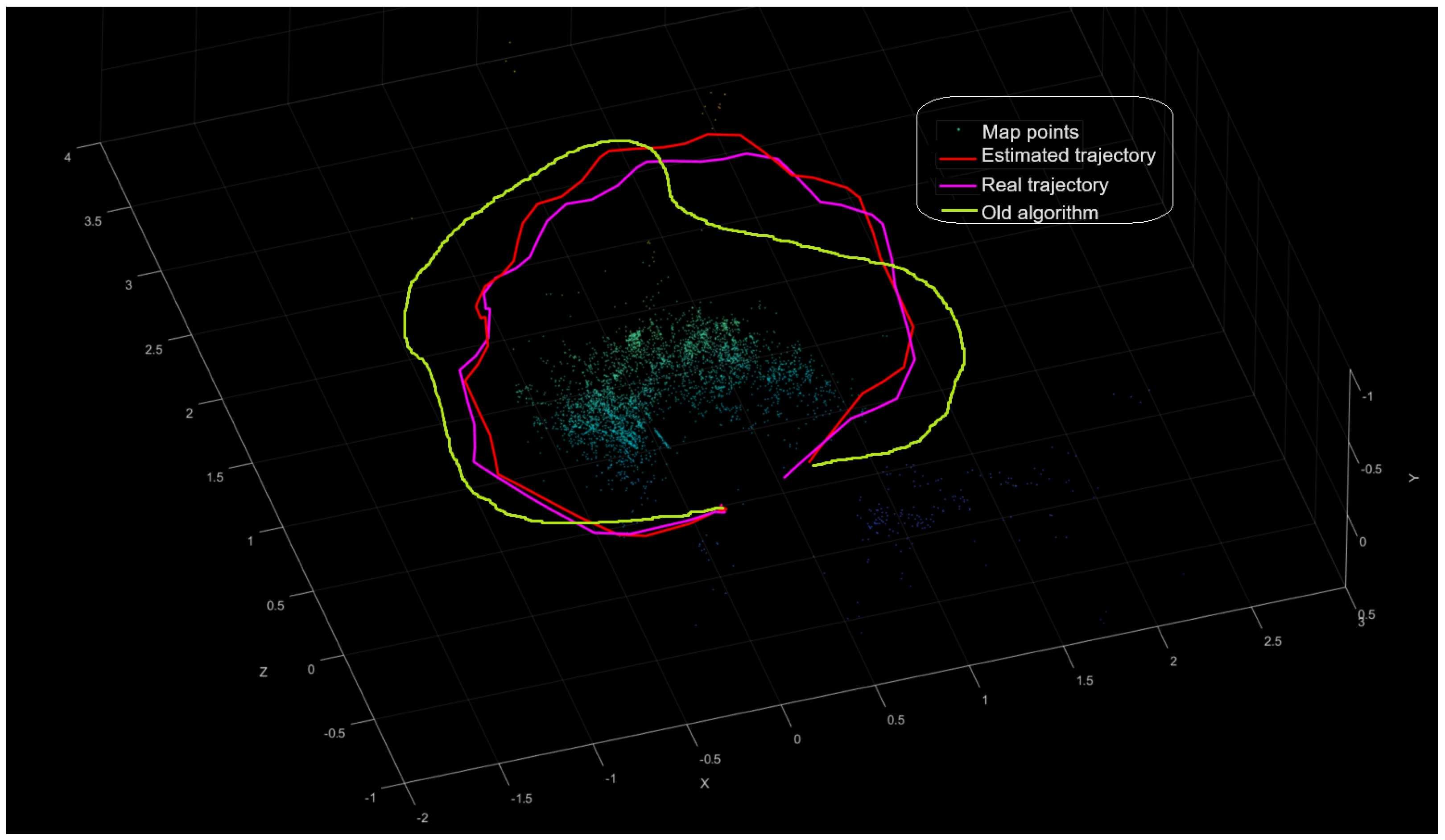
3.6. Compare with the Actual Camera Trajectory

This step involves comparing the estimated camera trajectory with the actual camera trajectory “ground truth positions ” to assess the accuracy of our algorithm. The actual camera trajectory is obtained from the ground truth poses of each frame. Figure 12 compares the estimated and actual camera trajectories, including all map points of the surrounding environment. The estimated keyframe trajectory achieves a low $RMSE$ of $0.20123$ using an adaptive threshold and parameter configuration. Meanwhile, the conventional algorithm with fixed parameters has a much higher $RMSE$ of $2.6907$.

4. Results and Analysis

This paper presented a novel adaptive ORB algorithm for VSLAM and demonstrated that using adaptive ORB parameters and an adaptive threshold improved tracking and mapping performance. Adaptive tuning enlarges the number of map points per frame, and the stringent adaptive threshold ensures robust tracking and mapping, which is helpful for autonomous UAV navigation. In contrast, traditional fixed-parameter methods (ORB-SLAM, ORB-SLAM2, VINS-Mono, FastORB-SLAM, and ORb-SLAM3) (such as scaleFactor, numLevels, and numPoints) perform well in well-defined conditions with minimal variability. However, adaptive parameters perform better in adaptive environments with frequent changes. Figure 13 shows the performance of the classical ORB algorithms in a dynamic environment, indicating how the algorithm struggled to precisely trace the route (failure in generating the route plot: b) and was even unable to precise tracking (defective path tracing with $RMSE$ being 3.280 as illustrated in plot (a)). The major drawback of the new method is the longer computational time caused by the use of adaptive parameters, which was generally longer compared to other methods. Under MATLAB experiments, the new method completed the entire process, comprising tracking, plotting uploaded ground truth, and comparing RMSE in about (03 min.15.56 s). The old ORB feature detection and extraction method performed the same process in approximately (02 min.19.59 s).

Table 1. RMSE and performance time for the adaptive method and the old algorithm in fixed and dynamic environments.

	RMSE to the Estimated Trajectory for Adapted ORB-SLAM	RMSE for the ORB-SLAM Fixed Parameters	Passed or Failed
Performance Time	03 min.15.56 s	02 min19.59 s
Daylight	RMSE: 0.20123	RMSE: 2.0697	Adaptive: 🗸 ORB-SLAM: 🗸
Extra Room Light	RMSE: 0.20123	RMSE: 2.0697	Adaptive: 🗸 ORB-SLAM: 🗸
Full Shading	RMSE: 0.20123	RMSE: 3.280	Adaptive: 🗸 ORB-SLAM: X
Half Shading	RMSE: 0.20123	RMSE: 2.5112	Adaptive: 🗸 ORB-SLAM: 🗸

shows the simulation results for RMSE and the performance time for the adaptive method and the ORB-SLAM algorithm in fixed and dynamic environments (changing lighting conditions—‘daylight, extra room light, full shading, and half shading’). The results for the adaptive method look to be more accurate, but it needed more time to execute. On the other hand, the different techniques are less precise and faster, or in full shading, and they failed to continue tracking the trajectory and closing the loop. From Table 1, the sign (🗸) refers to the method that succeeded in passing the test, closing the loop, and giving the full map, and the sign (X) refers to the failure to close the loop.

Table 2. Shows the eight experimental test results for fixed parameters of the ORB algorithm (Scale Factor, Num Levels, and Num Points) and threshold in the daylight.

Algorithm	Scale Factor	Num Levels	Num Points	Threshold	RMSE	Performance Time min-s
ORB-SLAM	1.2	8	600	40	2.0697	02 min19.59 s
Proposed Method	adaptive	adaptive	adaptive	adaptive	0.20123	03 min.15 s
ORB-SLAM2	1.5	8	1000	60	0.4523	02 min.15 s
VINS-Mono	1.7	7	900	60	0.4745	02 min.55 s
FORB-SLAM	1.3	7	856	60	0.4512	02 min.15 s
ORB-SLAM3	1.5	9	650	60	0.4756	02 min.12 s
DSO	/	/	/	/	0.3218	02 min.18 s
Test1(ORB-SLAM)	1.4	9	800	50	2.012	03 min.10 s
Test2(ORB-SLAM)	1.5	10	1000	55	1.9987	04 min.15 s
Test3(ORB-SLAM)	1.6	11	1200	60	1.898	03 min.50 s
Test4(ORB-SLAM)	1.3	12	1400	65	1.65	05 min.01 s
Test5(ORB-SLAM)	1.1	7	1600	70	1.82	04 min.08 s
Test6(ORB-SLAM)	1	6	2000	75	1.1154	02 min.40 s
Test7(ORB-SLAM)	0.9	13	2200	85	0.9987	02 min.56 s
Test8(ORB-SLAM)	0.8	15	2400	100	0.5548	02 min.50 s

shows the eight experimental test results for fixed parameters of the ORB algorithm (Scale Factor, Num Levels, and Num Points) and threshold, as well as the tests for the other algorithms (‘ORB-SLAM2-3, FastORB-SLAM, ORB-SLAM, and VINS-Mono’). Depending on the related reviews for visual SLAM algorithms [37], the performance of the V-SLAM methods varied in dynamic environments (changing lighting conditions—‘daylight, extra room light, full shading, and half shading’), and the performance weakened with low light because the parameters were fixed, resulting in fewer points being used for feature matching. The simulation results prove that the adaptive method has the most accurate performance in changing lighting conditions but has the longest execution time.

From Table 2, the experiments focus on comparing the performance of ORB-SLAM with the proposed method built on the ORB-SLAM platform and aimed at enhancing its performance under varying light conditions. The results show that while ORB-SLAM struggled with fixed parameter settings, particularly in dynamic scenes, the proposed adaptive method always recorded lower RMSE results, indicating improved accuracy in the estimation of the trajectory. Additionally, the tests illustrate the impact of different scale factors, levels, points, and threshold values on the performance of ORB-SLAM. As the number of points increased, the RMSE diminished consistently, albeit at the cost of increased processing time. The adaptive approach within the method of consideration selects optimal parameter values autonomously, with a compromise between accuracy and processing time. In addition, comparison with other state-of-the-art algorithms, such as ORB-SLAM2, VINS-Mono, and DSO, indicates that while these algorithms also returned low RMSE values, the proposed method beat them in adaptability under dynamic conditions. This is best depicted in Test8 (ORB-SLAM), where an optimized fixed-parameter method returned an RMSE of 0.5548, which is still higher than the proposed method’s 0.20123, depicting the advantage of adaptive optimization.

Table 3. Comparison between traditional ORB-SLAM and proposed adaptive ORB-SLAM.

Aspect	Traditional ORB-SLAM	Proposed Adaptive ORB-SLAM
Parameter Selection	Fixed values set manually before execution.	Adaptive parameters adjusted dynamically during runtime.
Robustness in Dynamic Environments	Struggles with changing lighting conditions, motion noise, and low-texture scenes.	Adapts automatically to different conditions, improving tracking stability.
Feature Extraction	Uses a fixed number of key points per frame.	Adjusts the number of key points dynamically based on scene complexity.
Computational Efficiency	Faster processing due to fixed parameters but less adaptive.	Slightly higher computational cost but significantly more accurate.
Tracking Performance	May lose tracking when key points are insufficient.	Re-extracts features dynamically, maintaining tracking accuracy.
Loop Closure and Mapping	Susceptible to drift due to static parameter settings.	More robust map generation with adaptive keyframe selection.
Real-time Applicability	Requires manual tuning for different environments.	Self-adjusting mechanism makes it suitable for real-time applications.
RMSE (Accuracy of Estimated Trajectory)	Higher RMSE due to parameter limitations.	Lower RMSE due to adaptive tuning.

compares the traditional ORB-SLAM with the proposed adaptive ORB-SLAM method. The traditional approach relies on fixed parameter values and is less efficient in dynamic scenes, low-texture environments, and varying lighting conditions. The proposed method, however, adapts important parameters dynamically at runtime, improving feature extraction, tracking resilience, and loop closure detection accuracy. Although the adaptive approach is slightly more computationally expensive, it significantly enhances the accuracy of the trajectory estimation by reducing RMSE and is more suitable for real-time UAV navigation.

Result Comparison with an Existing Adaptive Method

DynaSLAM [31] is a well-known adaptive SLAM method that performs effectively in environments with clearly distinguishable moving objects. However, it tends to underperform in low-light conditions due to its strong dependence on motion segmentation techniques. A comparative analysis between DynaSLAM and the proposed method is presented in

Table 4. Comparison between DynaSLAM and the proposed method.

Feature	DynaSLAM	Proposed Method (Adaptive ORB-SLAM)
Approach to Dynamic Environments	Removes moving objects using motion segmentation	Dynamically adjusts feature extraction and tracking parameters for better performance
Performance in Low-Light Conditions	Poor, as motion segmentation is sensitive to lighting and suffers from high noise	More robust, as an adaptive parameter tuning maintains performance in low-light scenarios
Effect on Generated Maps	Removes moving objects, which can lead to the loss of essential scene details	Does not remove elements but enhances the ability to track and adapt to them
Computational Cost	High due to motion detection and inpainting (background reconstruction)	Lower, as it focuses on improving parameters instead of removing objects
Real-Time Performance	Relatively slow, due to complex image processing operations	Slower but more efficient in real time, making it suitable for UAVs
Best Suited For	Environments with large moving objects, such as pedestrians and vehicles	Low-light or low-texture environments, where the feature extraction is more challenging
Reliability in Poor Lighting Conditions	Low, since poor lighting affects motion detection	High, as the method relies on the feature analysis rather than motion segmentation
RMSE (Accuracy of Estimated Trajectory)	Higher RMSE due to parameter limitations	Lower RMSE due to adaptive tuning.

. Unlike DynaSLAM, the proposed approach does not rely on detecting and removing dynamic objects. Instead, it dynamically adjusts SLAM parameters to suit the scene, which significantly enhances its robustness in challenging conditions such as low-light or low-texture environments. Moreover, DynaSLAM incurs a high computational cost due to the complexity of its image processing pipeline. In contrast, the proposed method is computationally more efficient, making it better suited for real-time applications and deployment on resource-constrained platforms such as UAVs. As a future direction, the integration of an FPGA accelerator is considered to address processing time limitations further.

5. Conclusions

This paper presented a novel method for enhancing the localization and mapping process in the Visual Simultaneous Localization and Mapping algorithm across various environments. This enhancement will improve the navigation of UAVs. The enhancement was achieved by using adaptive ORB parameters instead of fixed ones during the map initialization step. These parameters automatically adjust to achieve optimal detection and feature extraction. The results from this step are used in feature matching between frames, which is also optimized through an adaptive threshold. The experiment showed a root mean square error (RMSE) of around $0.20123$ for the key frame trajectory (in meters) compared to $2.6907$ for the previous algorithm that relied on fixed parameters. The proposed adaptive ORB algorithm is of key practical application in actual UAV navigation systems. The algorithm will be capable of automatically mapping crucial infrastructure in industrial spaces, such as power cables, pipelines, and buildings, particularly in GPS-denied zones. In military applications, the enhanced VSLAM method can be used to improve autonomous reconnaissance and surveillance operations in degraded or GNSS-denied environments. Furthermore, environmental monitoring operations, such as mapping hazardous areas or search-and-rescue missions in disaster zones, can be supported by the enhanced accuracy and reliability of the proposed method. Adaptive ORB can be easily integrated into UAV systems, since it is modular and compatible with typical visual sensors. Dynamically adjusting the most critical parameters of the algorithm implies that it can function optimally under different environmental conditions without manual calibration. This flexibility is beneficial in applications where UAVs must operate autonomously and in real time. The system can be implemented on embedded computing platforms with slight modifications to existing VSLAM frameworks, enabling practical deployment in UAV navigation pipelines.

Future Work

Future work will be aimed at reducing the computational complexity of the algorithm to allow implementation on low-power embedded devices. One promising direction is the implementation of the adaptive ORB method on an FPGA chip, which can utilize hardware parallelization to accelerate the feature extraction and matching process. In addition, future research can be done by including multi-sensor fusion techniques and combining visual cues with IMU and LIDAR data in order to enhance the precision of localization in challenging visual and dynamic environments. Additional extensions to support larger UAVs and more complex multi-agent systems will also be a significant area of concern, as will empirical evaluation of its performance on a broader set of real-world examples. By resolving these future directions, the adaptive ORB algorithm presented herein may significantly enhance autonomous UAV performance over a broad spectrum of applications, advancing operational effectiveness and environmental responsiveness.

References

1. Rostum, H.M.; Vásárhelyi, J. A Review of Using Visual Odometry Methods in Autonomous UAV Navigation in GPS-Denied Environment. Acta Univ. Sapientiae Electr. Mech. Eng. 2023, 15, 14–32. [Google Scholar]
2. Salih Omar, M.H.R.; Vásárhelyi, J. A Novel Method to Improve the Efficiency and Performance of Cloud-Based Visual Simultaneous Localization and Mapping. Eng. Proc. 2024, 79, 78. [Google Scholar] [CrossRef]
3. Chen, W.; Shang, G.; Ji, A.; Zhou, C.; Wang, X.; Xu, C.; Li, Z.; Hu, K. An overview on visual slam: From tradition to semantic. Remote Sens. 2022, 14, 3010. [Google Scholar] [CrossRef]
4. Mur-Artal, R.; Martinez Montiel, J.M.; Tardos, J.D. ORB-SLAM: A versatile and accurate monocular SLAM system. IEEE Trans. Robot. 2015, 31, 1147–1163. [Google Scholar] [CrossRef]
5. Engel, J.; Schöps, T.; Cremers, D. LSD-SLAM: Large-scale direct monocular SLAM. In Proceedings of the European Conference on Computer Vision, Zurich, Switzerland, 6–12 September 2014; Springer: Cham, Switzerland, 2014. [Google Scholar]
6. Mur-Artal, R.; Tardós, J.D. ORB-SLAM2: An open-source SLAM system for monocular, stereo, and RGB-D cameras. IEEE Trans. Robot. 2017, 33, 1255–1262. [Google Scholar] [CrossRef]
7. Qin, T.; Li, P.; Shen, S. VINS-Mono: A robust and versatile monocular visual-inertial state estimator. IEEE Trans. Robot. 2018, 34, 1004–1020. [Google Scholar]
8. Biber, P.; Strasser, W. The normal distributions transform: A new approach to laser scan matching. In Proceedings of the 2003 IEEE/RSJ International Conference on Intelligent Robots and Systems (IROS 2003), Las Vegas, NV, USA, 27 October–1 November 2003; IEEE Xplore: Piscataway, NJ, USA, 2003; Volume 3. [Google Scholar]
9. Singh, R.; Nagla, K.S. Comparative analysis of range sensors for the robust autonomous navigation—A review. Sens. Rev. 2019, 40, 17–41. [Google Scholar]
10. Cadena, C.; Carlone, L.; Carrillo, H.; Latif, Y.; Scaramuzza, D.; Neira, J.; Reid, I.; Leonard, J.J. Past, present, and future of simultaneous localization and mapping: Toward the robust-perception age. IEEE Trans. Robot. 2016, 32, 1309–1332. [Google Scholar]
11. Chen, C.; Wang, B.; Lu, C.X.; Trigoni, N.; Markham, A. A survey on deep learning for localization and mapping: Towards the age of spatial machine intelligence. arXiv 2020, arXiv:2006.12567. [Google Scholar]
12. Davison, A.J.; Reid, I.D.; Molton, N.D.; Stasse, O. MonoSLAM: Real-time single camera SLAM. IEEE Trans. Pattern Anal. Mach. Intell. 2007, 29, 1052–1067. [Google Scholar] [CrossRef] [PubMed]
13. Klein, G.; Murray, D. Parallel tracking and mapping for small AR workspaces. In Proceedings of the 2007 6th IEEE and ACM International Symposium on Mixed and Augmented Reality, Nara, Japan, 13–16 November 2007; IEEE Xplore: Piscataway, NJ, USA, 2007. [Google Scholar]
14. Strasdat, H.; Montiel, J.M.M.; Davison, A.J. Real-time monocular SLAM: Why filter? In Proceedings of the 2010 IEEE International Conference on Robotics and Automation, Anchorage, Alaska, 3 May 2010; IEEE Xplore: Piscataway, NJ, USA, 2010. [Google Scholar]
15. Rublee, E.; Rabaud, V.; Konolige, K.; Bradski, G. ORB: An efficient alternative to SIFT or SURF. In Proceedings of the 2011 International Conference on Computer Vision, Barcelona, Spain, 6–13 November 2011; IEEE Xplore: Piscataway, NJ, USA, 2011. [Google Scholar]
16. Kümmerle, R.; Grisetti, G.; Strasdat, H.; Konolige, K.; Burgard, W. g2o: A general framework for graph optimization. In Proceedings of the 2011 IEEE International Conference on Robotics and Automation, Shanghai, China, 9–13 May 2011; IEEE Xplore: Piscataway, NJ, USA, 2011. [Google Scholar]
17. Gálvez-López, D.; Tardos, J.D. Bags of binary words for fast place recognition in image sequences. IEEE Trans. Robot. 2012, 28, 1188–1197. [Google Scholar] [CrossRef]
18. Kurdel, P.; Novák Sedláčková, E.L.J. UAV flight safety close to the mountain massif. Transp. Res. Procedia 2019, 43, 319–327. [Google Scholar]
19. Pecho, P.; Velky, P.K.S.N.A. Use of Computer Simulation to Optimize UAV Swarm Flying; IEEE: Piscataway, NJ, USA, 2022; pp. 168–172. [Google Scholar]
20. Qin, T.; Shen, S. Robust initialization of monocular visual-inertial estimation on aerial robots. In Proceedings of the 2017 IEEE/RSJ International Conference on Intelligent Robots and Systems, Vancouver, BC, Canada, 24–28 September 2017; IEEE Xplore: Piscataway, NJ, USA, 2017. [Google Scholar]
21. Qin, T.; Cao, S.; Pan, J.; Shen, S. A general optimization-based framework for global pose estimation with multiple sensors. arXiv 2019, arXiv:1901.03642. [Google Scholar]
22. Cvišić, I.; Ćesić, J.; Marković, I.; Petrović, I. SOFT-SLAM: Computationally efficient stereo visual simultaneous localization and mapping for autonomous unmanned aerial vehicles. J. Field Robot. 2018, 35, 578–595. [Google Scholar] [CrossRef]
23. Tateno, K.; Tombari, F.; Laina, I.; Navab, N. CNN-SLAM: Real-time dense monocular SLAM with learned depth prediction. In Proceedings of the IEEE Conference on Computer Vision and Pattern Recognition, Honolulu, HI, USA, 21–26 July 2017; IEEE Xplore: Piscataway, NJ, USA, 2017. [Google Scholar]
24. Newcombe, R.A.; Lovegrove, S.J.; Davison, A.J. DTAM: Dense tracking and mapping in real-time. In Proceedings of the 2011 International Conference on Computer Vision, Barcelona, Spain, 6–13 November 2011; IEEE Xplore: Piscataway, NJ, USA, 2011. [Google Scholar]
25. Newcombe, R.A.; Izadi, S.; Hilliges, O.; Molyneaux, D.; Kim, D.; Davison, A.J.; Kohi, P.; Shotton, J.; Hodges, S.; Fitzgibbon, A. Kinectfusion: Real-time dense surface mapping and tracking. In Proceedings of the 2011 10th IEEE International Symposium on Mixed and Augmented Reality, Basel, Switzerland, 26–29 October 2011; IEEE Xplore: Piscataway, NJ, USA, 2011. [Google Scholar]
26. Usenko, V.; Demmel, N.; Schubert, D.; Stückler, J. Visual-inertial mapping with non-linear factor recovery. IEEE Robot. Autom. Lett. 2019, 5, 422–429. [Google Scholar]
27. Engel, J.; Sturm, J.; Cremers, D. Semi-dense visual odometry for a monocular camera. In Proceedings of the IEEE International Conference on Computer Vision, Vancouver, BC, Canada, 7–14 July 2001; IEEE Xplore: Piscataway, NJ, USA, 2013. [Google Scholar]
28. Forster, C.; Pizzoli, M.; Scaramuzza, D. SVO: Fast semi-direct monocular visual odometry. In Proceedings of the 2014 IEEE International Conference on Robotics and Automation (ICRA), Hong Kong, China, 31 May–7 June 2014; IEEE Xplore: Piscataway, NJ, USA, 2014. [Google Scholar]
29. Fischler, M.A.; Bolles, R.C. Random sample consensus: A paradigm for model fitting with applications to image analysis and automated cartography. Commun. ACM 1981, 24, 381–395. [Google Scholar] [CrossRef]
30. Yu, C.; Liu, Z.; Liu, X.J.; Xie, F.; Yang, Y.; Wei, Q.; Fei, Q. DS-SLAM: A semantic visual SLAM towards dynamic environments. In Proceedings of the 2018 IEEE/RSJ International Conference on Intelligent Robots and Systems (IROS), Madrid, Spain, 1–5 October 2018; IEEE Xplore: Piscataway, NJ, USA, 2018. [Google Scholar]
31. Bescos, B.; Fácil, J.M.; Civera, J.; Neira, J. DynaSLAM: Tracking, mapping, and inpainting in dynamic scenes. IEEE Robot. Autom. Lett. 2018, 3, 4076–4083. [Google Scholar] [CrossRef]
32. Bârsan, I.A.; Liu, P.; Pollefeys, M.; Geiger, A. Robust dense mapping for large-scale dynamic environments. In Proceedings of the 2018 IEEE International Conference on Robotics and Automation (ICRA), Brisbane, Australia, 21–25 May 2018; IEEE Xplore: Piscataway, NJ, USA, 2018. [Google Scholar]
33. Yang, D.; Bi, S.; Wang, W.; Yuan, C.; Wang, W.; Qi, X.; Cai, Y. DRE-SLAM: Dynamic RGB-D encoder SLAM for a differential-drive robot. Remote Sens. 2019, 11, 380. [Google Scholar] [CrossRef]
34. Dou, M.; Khamis, S.; Degtyarev, Y.; Davidson, P.; Fanello, S.R.; Kowdle, A.; Escolano, S.O.; Rhemann, C.; Kim, D.; Taylor, J.; et al. Fusion4d: Real-time performance capture of challenging scenes. ACM Trans. Graph. (ToG) 2016, 35, 1–13. [Google Scholar]
35. Rünz, M.; Agapito, L. Co-fusion: Real-time segmentation, tracking and fusion of multiple objects. In Proceedings of the 2017 IEEE International Conference on Robotics and Automation (ICRA), Singapore, 29 May–3 June 2017; IEEE Xplore: Piscataway, NJ, USA, 2017. [Google Scholar]
36. Shao, S. A Monocular SLAM System Based on the ORB Features. In Proceedings of the 2023 IEEE 3rd International Conference on Power, Electronics and Computer Applications (ICPECA), Shenyang, China, 29–31 January 2023; IEEE Xplore: Piscataway, NJ, USA, 2023. [Google Scholar]
37. Macario Barros, A.; Michel, M.; Moline, Y.; Corre, G.; Carrel, F. A comprehensive survey of visual slam algorithms. Robotics 2022, 11, 24. [Google Scholar] [CrossRef]
Figure 1. The scheme of feature-based VSLAM algorithm [2].
Electronics 14 01440 g001
Figure 2. The DJI Tello drone; Ryze Tech, Shenzhen, China (in collaboration with DJI, Dà-Jiāng Innovations, Shenzhen, China). used in the experiments.
Electronics 14 01440 g002
Figure 3. Image of the database used in the experiment.
Electronics 14 01440 g003
Figure 4. The image of the first frame from the database and the start point.
Electronics 14 01440 g004
Figure 5. Example of corners, edges, keypoints, and blocks.
Electronics 14 01440 g005
Figure 6. How ORB feature extraction works (OpenCV Website (https://docs.opencv.org/4.x/df/d0c/tutorial_py_fast.html, access date: 31 March 2025)).
Electronics 14 01440 g006
Figure 7. Adapted ORB detection and extraction flow chart.
Electronics 14 01440 g007
Figure 8. Image of keypoints (output) obtained by adaptive ORB algorithm.
Electronics 14 01440 g008
Figure 9. The image of the process of matching features between two sequential frames.
Electronics 14 01440 g009
Figure 10. Image of map points and camera locations from the simulation process.
Electronics 14 01440 g010
Figure 11. Image of path tracking and mapping.
Electronics 14 01440 g011
Figure 12. A graphical comparison between the estimated trajectory and the ground truth camera path.
Electronics 14 01440 g012
Figure 13. Graphs presenting the failure of the old algorithms to estimate the trajectory: (a) Optimized fixed parameters in a dynamic environment. (b) Fixed parameters in a dynamic environment.
Electronics 14 01440 g013