Article

Enhancing Out-of-Distribution Detection Under Covariate Shifts: A Full-Spectrum Contrastive Denoising Framework

Computer Engineering and Science Department, Shanghai University, Shanghai 200444, China
*
Author to whom correspondence should be addressed.
Electronics 2025, 14(9), 1881; https://doi.org/10.3390/electronics14091881
Submission received: 2 April 2025 / Revised: 28 April 2025 / Accepted: 5 May 2025 / Published: 6 May 2025

Abstract

Out-of-distribution (OOD) detection is crucial for identifying samples that deviate from the training distribution, thereby enhancing the reliability of deep neural network models. However, existing OOD detection methods primarily address semantic shifts, where an image’s inherent semantics have changed, and often overlook covariate shifts, which are prevalent in real-world scenarios. For instance, variations in image contrast, lighting, or viewpoints can alter input features while keeping the semantic content intact. To address this, we propose the Full-Spectrum Contrastive Denoising (FSCD) framework, which improves OOD detection under covariate shifts. FSCD first establishes a robust semantic boundary and then refines feature representations through fine-tuning. Specifically, FSCD employs a dual-level perturbation augmentation module to simulate covariate shifts and a feature contrastive denoising module to effectively distinguish in-distribution samples from OOD samples. Extensive experiments on three benchmarks demonstrate that FSCD achieves state-of-the-art performance, with AUROC improvements of up to 0.51% on DIGITS, 0.55% on OBJECTS, and 2.09% on COVID compared to the previous best method while also maintaining the highest classification accuracy on covariate-shifted in-distribution samples.

1. Introduction

Deep neural networks have been widely deployed and have achieved exceptional performance in a variety of applications, such as classification, object detection, and semantic segmentation [1,2,3]. However, when the models encounter samples that were not present during training, they may confidently misclassify them as known classes, leading to a significant deterioration in performance [4]. With the growing demand for intelligent detection technologies, robust models must handle out-of-distribution (OOD) inputs. This necessity has driven the development of out-of-distribution detection methods [5,6], which focus on identifying inconsistencies between training and test data.
However, the traditional setup of out-of-distribution detection still relies on the unrealistic assumption that test data only exhibit semantic shifts, overlooking the fact that in-distribution data can also undergo covariate shifts. Covariate shifts refer to changes in the statistical properties of data when the underlying semantics remain consistent. As shown in Figure 1, covariate shifts are prevalent in real-world scenarios, such as image style, noise, lighting, or viewpoints.
Zhang et al. [7] observed that out-of-distribution detection algorithms, which are designed considering only semantic shifts, suffer significant performance degradation when faced with covariate shifts. This degradation is mainly reflected in two aspects: failure to classify in-distribution (ID) samples under covariate shifts, and the tendency to misidentify them as OOD samples.
To tackle this issue, Yang et al. [8] first introduced the concept of Full-Spectrum Out-of-Distribution Detection (Fs-OOD). In the Fs-OOD task, the model encounters OOD data and ID data under covariate shifts during testing. The model is expected to classify samples exhibiting only semantic shifts as OOD while accurately identifying and classifying ID samples. Fs-OOD aims to enhance the model’s robustness against various distribution changes, ensuring high performance across a wide range of practical applications.
Although several studies [8,9,10,11,12] have discussed covariate shifts, there is still no consensus on how to classify covariate-shifted samples. Some researchers argue that they should be considered as OOD due to their deviating distributions, while others contend that they should be excluded from OOD detection since the primary goal is to differentiate between semantic shifts. In this paper, we argue that the full-spectrum out-of-distribution detection setup is more practical, as it realistically simulates real-world conditions and enables a more comprehensive evaluation of model performance in challenging scenarios.
To address the challenge of out-of-distribution detection under covariate shifts, we propose the Full-Spectrum Contrastive Denoising (FSCD) framework. In contrast to SEM, which employs the corresponding semantic scoring function, FSCD employs a two-stage learning process—a semantic initialization stage and a fine-tuning stage—to effectively distinguish covariate-shifted ID samples from OOD samples. In the semantic initialization stage, the outlier exposure strategy is used to jointly optimize in-distribution data and auxiliary outlier samples, establishing an initial semantic decision boundary. The fine-tuning stage relies on two key components: a dual-level perturbation augmentation (DLPA) module and a feature contrastive denoising (FCD) module. DLPA introduces perturbations at both image and feature levels to enhance sample diversity and simulate covariate shifts. Meanwhile, FCD first performs dimensionality reduction to denoise perturbed ID data and then leverages contrastive learning at the feature level to enforce semantic consistency between original and perturbed data, thereby improving the separability of ID and OOD samples in the feature space. Our proposed method (FSCD) not only improves the model’s ability to handle covariate shifts but also enhances its capacity to distinguish OOD samples, marking a substantial step forward from SEM in the realm of FS-OOD detection.
The main contributions of this work are as follows:
  • We propose the Full-Spectrum Contrastive Denoising (FSCD) framework, which integrates semantic boundary initialization with fine-tuning, significantly improving OOD detection performance in scenarios with covariate shifts.
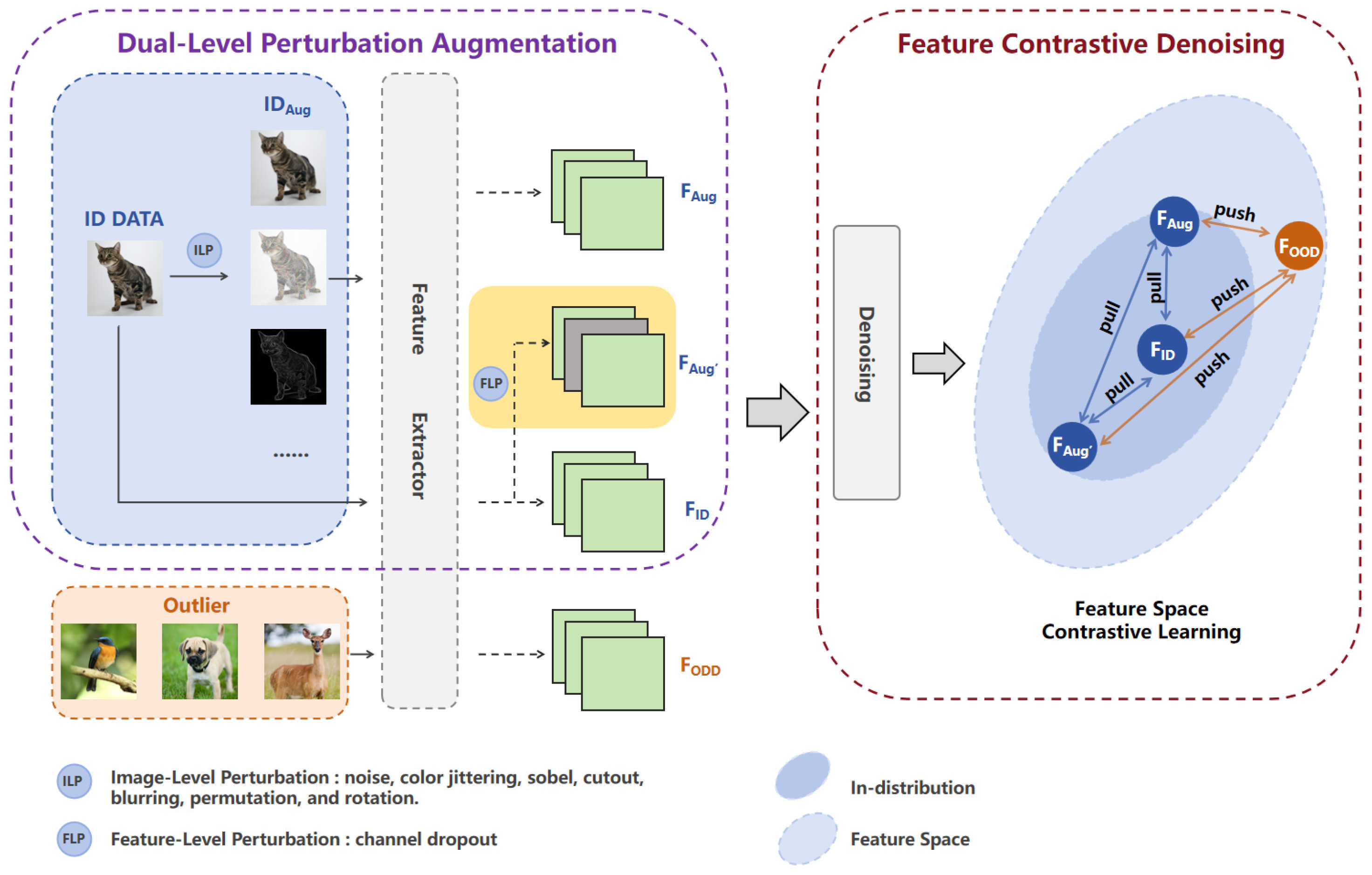
  • We propose the dual-level perturbation augmentation (DLPA) and feature contrastive denoising (FCD) modules to simulate complex covariate shifts and enable more granular differentiation of samples, thereby enhancing the model’s adaptability to distributional variations.
  • The effectiveness and superiority of FSCD are validated through extensive experiments on multiple datasets, demonstrating its advantages over existing approaches in full-spectrum out-of-distribution detection and providing new insights for future research.
The structure of this paper is outlined as follows. Section 2 provides a review of existing research on out-of-distribution detection and covariate shifts, introducing recent advancements in the field and the key challenges they face. Section 3 introduces the proposed method FSCD, detailing its architecture, the dual-level perturbation augmentation module, and the feature contrastive denoising module. Section 4 presents comprehensive experimental results after evaluating FSCD on three benchmarks—DIGITS, OBJECTS, and COVID—demonstrating its state-of-the-art performance. Section 5 discusses the limitations of the approach presented in this paper and provides an outlook on possible future research directions. The conclusions are presented in Section 6.

2. Related Works

2.1. Out-of-Distribution Detection

Current methodologies in out-of-distribution detection primarily fall into two categories [13]: training-based methods and post hoc inference methods.
Training-based approaches enhance OOD awareness by explicitly integrating OOD considerations into the training process. A widely used training-based method is outlier exposure (OE) [14], which leverages the abundance of real-world unlabeled data that do not overlap with the in-distribution data. These samples form a broadly defined auxiliary outlier dataset for training. OE trains models with auxiliary OOD data by jointly optimizing with both outlier and ID samples. By exposing the model to outliers, OE encourages a more conservative inlier representation, thereby improving the detection of novel anomalies. Several studies proposed further refinements of OE-based training. OECC [15] introduces confidence calibration for outliers to improve score reliability. MixOE [16] optimizes outlier mixing ratios through gradient alignment, while BERL [17] enforces balanced regularization across different classes. Additionally, there exists a class of methods that do not require outlier data during training. For instance, SCALE [18] extends the application of scaling to the training phase, introducing an enhancement method that significantly improves OOD detection.
Post hoc inference methods boost the separation between ID and OOD by developing score functions during the inference stage. They range from the baseline maximum softmax probability (MSP) [5] to more advanced techniques. ODIN [19] enhances detection by applying temperature scaling and input perturbations to the softmax scores, while EBO [20] utilizes the energy score derived from logits to distinguish OOD samples. ReAct [21] introduces a thresholding mechanism on feature activations to improve OOD detection, and Maximum Logit Score [22] focuses on the highest logit value for detection purposes. ATS [23] dynamically calculates a temperature value based on activations of the intermediate layers, while ExCeL [24] combines extreme and collective information within the output layer for enhanced OOD detection.
Despite notable advancements in out-of-distribution detection techniques, current methods often struggle to effectively handle scenarios involving covariate shifts. Addressing this challenge is crucial for enhancing model reliability in real-world applications.

2.2. Solutions to Covariate Shifts

A semantic shift refers to variations at the category or label level, altering the intrinsic meaning of data. In contrast, covariate shift occurs when the input distribution changes while the underlying labels remain unchanged. A typical example of a covariate shift in image processing is dehazing. Zhang et al. [25] proposed a generative adversarial and self-supervised dehazing network that uses GANs and self-supervised learning to enhance performance on natural hazy images and reduce domain shifts. Similarly, VNDHR [26] tackles nighttime haze challenges using hybrid regularization to improve illumination and reflectance. These approaches show how covariate shifts can be addressed by enhancing model generalization, thereby improving performance across various environmental conditions and image degradations.
Although many existing studies in OOD detection have discussed covariate shifts, their definitions and focus differ from those in the full-spectrum OOD detection setting. For example, ODIN [9] demonstrated that OOD samples exhibiting both semantic and covariate shifts are easier to detect than those with only one type of shift. Their work specifically examined covariate-shifted OOD samples. CSI [27] introduces augmented samples mainly for contrastive training and treats some of the augmented samples as negative examples, which is inconsistent with the definition of covariate shift in full-spectrum OOD detection. Yang et al. [8] formally introduced the full-spectrum OOD detection framework, which categorizes samples with semantic shifts as OOD, while ID samples undergoing covariate shifts are expected to be recognized as ID and correctly classified. They also proposed a semantic scoring function, SEM, comprising two probabilistic measures: one derived from high-level features that encode both semantic and non-semantic information, and another from low-level feature statistics that capture only stylistic attributes. By combining these measures, the non-semantic component is effectively eliminated, yielding a score that solely reflects semantic information. Long et al. [10] proposed an incremental shift OOD evaluation method, partitioning test samples by semantic and covariate shift intensity for refined assessment. Kyungpil [28] utilizes an adversarial mixup training method to synthesize OOD samples and evaluate OOD generalization using a distance-aware detector. Averly [11] further emphasized that the boundary between in-distribution and OOD samples is inherently model-dependent. In this paper, we follow the same experimental setup as SEM, while proposing a more robust framework that improves upon their approach through enhanced modeling and algorithmic design.
Another line of work argues that test datasets should exclude covariate-shifted samples to maintain the fundamental goal of OOD detection. A clean ImageNet-OOD dataset [12] was created to support this perspective, which only has semantic shifts to ensure a more controlled evaluation environment.
However, the setup of Fs-OOD holds greater practical significance, particularly in applications such as autonomous driving, where environmental variations, such as illumination changes, seasonal vegetation differences, and weather conditions, must be accounted for to ensure reliable decision-making. This paper adopts the same setting.

3. Proposed Method

3.1. Overall Architecture

The proposed FSCD framework is based on the concept of outlier exposure and consists of two stages: semantic boundary initialization and fine-tuning.
In the semantic boundary initialization stage, also referred to as the pretraining stage, the model is trained on both ID samples and auxiliary outlier data to establish an initial classification boundary and capture the semantic features of each class. The primary objective during this stage is to learn fundamental classification abilities.
The fine-tuning stage is specifically designed for the Fs-OOD task, as shown in Figure 2. In this phase, the input consists of in-distribution samples, auxiliary outliers, and augmented ID samples generated via both image-level and feature-level perturbations. These samples are passed through a shared feature extractor to obtain the corresponding feature representations: F ID for clean ID data, F Aug for image-perturbed samples, F Aug for feature-perturbed samples, and F OOD for outliers.
Since perturbations may introduce noise into ID representations, FSCD first applies feature denoising to suppress redundant low-level variations. Then, contrastive learning is employed to align F ID , F Aug , and F Aug while enforcing separation from F OOD . This combination of denoising and contrastive learning encourages semantic consistency across perturbed variants and improves the model’s ability to discriminate between in- and out-of-distribution samples under covariate shifts.

3.2. Semantic Boundary Initialization Stage

During the semantic boundary initialization stage, FSCD leverages both in-distribution samples and auxiliary outliers to learn a robust semantic classification boundary. This stage corresponds to a standard classifier pretraining process, in which the model is trained to accurately predict class labels for ID samples while simultaneously learning to reject outliers by assigning them to a designated rejection class. Although conceptually simple, this stage is essential for providing a strong initialization that facilitates subsequent perturbation modeling and contrastive denoising efforts. This phase enables the model to acquire a fundamental classification capability and form a coarse semantic separation between ID and OOD data in the feature space, laying the foundation for the fine-tuning stage.
The optimization objective in this stage is defined as follows. A rejection class [29,30] for outliers is introduced as the ( N + 1 ) -th class, where N denotes the number of ID categories and x represents the outlier samples drawn from the auxiliary outlier training set D out train . denotes the cross-entropy loss for classification, f ( x ) is the predicted probability distribution for input x, and y is the ground-truth label for the ID samples. The set D in train denotes the in-distribution training set, and the hyperparameter λ balances the loss components, ensuring a trade-off between accurate classification of ID data and reliable detection of outliers.
L SBI = E ( x , y ) D in train ( f ( x ) , y ) + λ · E x D out train [ ( f ( x ) , N + 1 ) ]

3.3. Fine-Tuning Stage

The fine-tuning stage consists of two key modules: dual-level perturbation augmentation (DLPA) and feature contrastive denoising (FCD), designed to enhance the model’s ability to distinguish covariate-shifted ID samples from OOD samples. The following sections detail the composition, functionality, and optimization objectives of each module.

3.3.1. Dual-Level Perturbation Augmentation Module

To address the misclassification of in-distribution samples that are affected by covariate shifts, we propose DLPA.
In the full-spectrum OOD detection setting, models are expected to handle a wide range of unknown distribution shifts during testing, which makes it impractical to rely on a specific optimization objective for generating samples. Instead, DLPA applies a variety of perturbations directly to training samples, mimicking real-world covariate shifts in a non-parametric, augmentation-based manner. As illustrated in Figure 2, DLPA introduces perturbations to in-distribution samples at both the image and feature levels [27,31,32]. The primary objective is to generate a diverse set of perturbed samples, which enhances the model’s ability to generalize across various covariate shifts. By exposing the model to a broad range of perturbations, DLPA facilitates a more comprehensive understanding of data variations, improving its robustness against complex distribution shifts.
At the image level, DLPA builds upon the setup of CSI [27] and applies a series of data augmentation techniques, including noise, color jittering, cutout, Sobel, blurring, permutation, and rotation. While CSI argues that certain augmentations may distort the original data distribution, we contend that they effectively preserve the core semantic information of in-distribution samples while simulating diverse covariate shifts. For instance, Gaussian noise is introduced to model sensor noise and environmental interference, while color jittering randomly adjusts hue, saturation, and brightness to account for variations in lighting conditions and imaging devices. Brightness adjustment alters overall luminance, simulating changes in ambient lighting. By incorporating these perturbations, DLPA significantly enhances training diversity, improving the model’s robustness to real-world covariate shifts.
After the image-level perturbation, the samples are processed through the feature extractor and subjected to feature-level perturbation. It should be noted that simple channel dropout performs sufficiently well [31,32], so we apply it to feature representations to enhance robustness. This regularization strategy encourages the model to learn more discriminative and invariant features, effectively widening its decision boundaries in the feature space.
DLPA retains a clean branch for PCA-based dimensionality reduction and denoising training, serving as a supervision signal for learning stable representations. It applies perturbations at different levels separately on the clean ID branch, rather than applying feature perturbations to already perturbed data, ensuring independent operation on the clean branch. This design allows the model to accurately capture the effects of perturbations, thereby enhancing robustness and generalization. After processing through DLPA, the final outputs consist of the original in-distribution features F ID ; the feature-perturbed representations F Aug , which capture transformations in the feature space; and the image-perturbed representations F Aug , which reflect variations in visual appearance. This structured perturbation strategy strengthens generalization on in-distribution samples, ensuring stable performance under complex shifts.

3.3.2. Feature Contrastive Denoising Module

FCD is designed to enhance the model’s robustness against ID perturbations while improving its capacity to distinguish OOD samples. By leveraging both feature denoising and contrastive learning, FCD facilitates a more structured and discriminative feature representation.
During the denoising phase, a dimensionality reduction technique is applied to filter out perturbational noise while preserving essential semantic information. While high-dimensional features extracted from deep networks contain rich class-discriminative cues, they also capture irrelevant variations and noise, particularly in perturbed ID samples. To address this, we use Principal Component Analysis (PCA) to project features onto a lower-dimensional subspace that retains high-variance components while filtering out low-variance directions associated with noise. Specifically, we retain 99% of the total variance to ensure that only the most informative components are preserved. To avoid interference from OOD samples, the transformation is learned exclusively from clean ID features, ensuring a more reliable representation of in-distribution variation.
To refine feature representations, we incorporate contrastive learning into Fs-OOD. By constructing positive and negative sample pairs, this method promotes feature consistency for ID samples while maximizing the separation between ID and OOD distributions. We define three optimization objectives to govern the relationships among ID, perturbed ID, and OOD samples. First, the model minimizes the feature distance between an ID sample and its perturbed counterpart to learn invariant features. Second, it maximizes the feature distance between the perturbed ID and OOD samples, as well as between the ID and OOD samples, ensuring clear distributional boundaries. This structured optimization improves the model’s generalization to unseen data distributions, enhancing detection accuracy and robustness in dynamic environments.
The loss function L CD builds upon the conventional L2 loss [33] by introducing a margin constraint for negative sample pairs. This loss encourages alignment between the ID samples and their perturbed variants (positive pairs) while enforcing a minimum margin on negative pairs (ID/OOD and perturbed/OOD) when their feature distances fall below a threshold. The mathematical formulation is given by
L CD = E x D in train f ( x ) f G aug ( x ) 2 2 k · ( E x D in train x D out train max 0 , m f ( x ) f ( x ) 2 2 + E x D in train x D out train max 0 , m f G aug ( x ) f ( x ) 2 2 ) .
Here, G aug denotes the augmentation function applied to the input data, and m represents the margin threshold, which is a hyperparameter that determines the minimum distance that features of negative sample pairs should maintain. The parameter k is a scaling factor that controls the relative importance of the second term.
Since one of the primary objectives in OOD detection is to maintain classification accuracy on in-distribution samples, the fine-tuning phase continues to incorporate classification learning for ID data. The overall loss function L FT for the fine-tuning phase is formulated as
L FT = E ( x , y ) D in train ( f ( x ) , y ) + λ 1 · L CD .
The parameter λ 1 is a scaling factor that controls the relative weight between the classification loss and the contrastive denoising loss during the fine-tuning phase. The total optimization objective, while preserving ID classification accuracy, enforces compact feature representations for ID samples and ensures sufficient separation from OOD samples, thereby enhancing the model’s discriminative power and robustness to distribution shifts.

4. Experiments

In this section, we first introduce the implementation of the experiments, providing a detailed description of the datasets, experimental settings, and evaluation metrics. Subsequently, we report the experimental results of the proposed algorithm on several standard benchmark datasets. To further validate the effectiveness of the proposed modules, systematic ablation studies are conducted, alongside an in-depth analysis of key hyperparameters.

4.1. Datasets

Following the settings in SEM [8], this section conducts experiments on three full-spectrum OOD detection benchmarks: DIGITS, OBJECTS, and COVID. Unlike conventional OOD evaluations, the ID test set includes covariate shift datasets, which share the same class labels and semantic features as the ID data but differ in collection methods, image styles, and statistical characteristics.
DIGITS: The ID dataset of DIGITS is MNIST [34], a grayscale handwritten digit dataset. The ID test set comprises the original MNIST test set along with covariate-shifted samples from SVHN and USPS [35]. SVHN consists of digit images captured from house number plates in real-world scenes, introducing variations in background, illumination, and orientation. The USPS dataset, collected from postal mail, features diverse handwriting styles and smaller image dimensions, which pose additional challenges for recognition. The OOD test set includes notMNIST and FashionMNIST [36], which share visual similarities with MNIST. The OOD test set also includes Texture [37], CIFAR-10 [38], Tiny-ImageNet [39], and Places365 [40], which exhibit distinct semantic and structural differences.
OBJECTS: The ID dataset is CIFAR-10 [38], which contains color images from 10 object categories. The ID test set includes the standard CIFAR-10 test set along with covariate-shifted samples from CIFAR-10-C and ImageNet-10 [41]. CIFAR-10-C introduces various corruption types (e.g., noise, blur, and contrast changes) at different severity levels, simulating real-world degradation. ImageNet-10 consists of fine-grained categories from ImageNet-22K that semantically correspond to CIFAR-10 classes. The OOD test set includes CIFAR-100, Tiny-ImageNet, MNIST, FashionMNIST, Texture, and CIFAR-100-C.
COVID: This benchmark evaluates OOD detection in medical imaging. The ID dataset is BIMCV [42], a lung X-ray dataset. The covariate shift test set is introduced using ActMed [43] and Hannover [44], which contain X-ray images collected from different hospitals. The OOD test set includes CT-SCAN [45], XRayBone [46], MNIST, CIFAR-10, Texture, and Tiny-ImageNet.
Auxiliary outlier training set: TinyImages80M [47] is utilized as the auxiliary outlier training set, designated as D out train . It is an image classification dataset provided by Stanford University. As a reduced version of ImageNet, it has become a popular benchmark due to its relatively small scale and diverse class distribution. Since CIFAR-10 and CIFAR-100 are labeled subsets of the TinyImages80M dataset, we follow the same deduplication procedure as in [9] and remove images from the dataset that belong to CIFAR-10 or CIFAR-100.

4.2. Experimental Settings

For the network architecture, appropriate structures were chosen for different benchmarks. Specifically, LeNet-5 was utilized for the DIGITS benchmark, while ResNet-18 was adopted for both the OBJECTS and COVID benchmarks. All models were trained using the stochastic gradient descent (SGD) optimizer with a momentum of 0.9 and a weight decay of 5 × 10 4 . For the DIGITS and OBJECTS benchmarks, the initial learning rate was set to 0.1 and was gradually decayed using a cosine annealing schedule over a total of 100 training epochs. For the COVID benchmark, the initial learning rate was set to 0.001, and the total number of training epochs was increased to 200 to accommodate the higher complexity of this benchmark. Additionally, during the fine-tuning phase, the learning rate was adjusted to 0.005, and the total number of fine-tuning epochs was set to 10. A fixed batch size of 128 was used across all benchmarks to balance computational efficiency and performance.
For hyperparameter configuration, we followed the commonly used values in outlier exposure methods. Specifically, λ was set to 0.5, λ 1 was set to 0.3, and k was set to 0.5. For the parameter m, a dynamic calculation strategy was employed: within each batch, the feature distances for different sample pairs were computed, and the 95th percentile was selected as the threshold to adapt to changes in the feature distribution. In particular, two types of feature distances were computed: one between the perturbed samples and the OOD samples, and another between the ID samples and the OOD samples; the maximum of these two distances was then taken as the final threshold.
In the experiments, we compared FSCD with several representative OOD detection methods, including MSP [5], EBO [20], MDS [48], ViM [49], IPL [50], and the current state-of-the-art approach, SEM [8]. MSP is a widely adopted baseline that detects OOD samples based on the maximum softmax probability. Despite its simplicity, it remains a strong and effective reference method due to its practicality and broad applicability. EBO distinguishes OOD samples using energy scores computed from the model’s logits. Incorporating temperature scaling and employing negative energy as the detection metric alleviates the overconfidence issue commonly observed in deep neural networks. MDS introduces a generative classifier under the linear discriminant analysis (LDA) assumption. It models class-conditional Gaussian distributions over both lower- and higher-level features of deep networks and defines a confidence score based on the Mahalanobis distance, effectively capturing feature-space deviations of OOD inputs. ViM uses a novel scoring strategy termed Virtual-logit Matching, which combines a class-agnostic component from the feature space with class-dependent logits. This hybrid formulation enhances OOD detection by jointly modeling semantic similarity and uncertainty. IPL is a novel method that identifies and concentrates on intrinsic parameters that capture semantic correlations, while reducing the negative impacts of covariance overfitting, to boost the model’s robustness and generalization in OOD detection tasks. SEM, the most recent and relevant method, formally introduces the full-spectrum OOD detection task. In our experiments, we conducted comprehensive comparisons with SEM to demonstrate the advantages and robustness of FSCD under various covariate and semantic shift scenarios.

4.3. Evaluation Metrics

To rigorously evaluate the efficacy of full-spectrum out-of-distribution detection, we employed four widely recognized metrics: the Area Under the Receiver Operating Characteristic Curve (AUROC), the Area Under the Precision–Recall Curve (AUPR), the false positive rate at a 95% true positive rate (FPR95), and accuracy (ACC) on the ID test set, including covariate-shifted samples. AUROC measures the model’s ability to distinguish between classes by plotting the true positive rate against the false positive rate at various threshold settings, while AUPR focuses on the trade-off between precision and recall, providing a more informative view of performance for imbalanced datasets. FPR95 quantifies the false positive rate when the true positive rate reaches 95%, offering insight into model specificity. ACC evaluates the model’s accuracy on the ID test set, reflecting its generalization ability under distribution shifts. A robust model is expected to achieve high AUROC and AUPR values and a low FPR95 value and maintain an ACC comparable to standard ID performance.

4.4. Results and Analysis

Overall, our proposed FSCD effectively distinguished various OOD datasets, achieving excellent performance in both Near-OOD tasks, where the OOD samples were similar to the ID samples, and Far-OOD tasks, where the style and content differed significantly from the ID samples. In particular, FSCD outperformed existing approaches on the AUROC and AUPR metrics across all benchmarks. Furthermore, compared to SEM, FSCD exhibited a lower FPR95, indicating enhanced robustness in OOD detection.
Table 1 compares the proposed FSCD method with existing methods for full-spectrum OOD detection using the AUROC metric. FSCD achieved state-of-the-art performance across all three benchmarks, attaining mean AUROC scores of 76.49%, 78.07%, and 90.11% on the DIGITS, OBJECTS, and COVID datasets, respectively, consistently outperforming previous approaches. Notably, FSCD demonstrated a balanced superiority in both Near-OOD and Far-OOD scenarios. It improved the AUROC by 0.73–1.45% over the second-best method (SEM) on DIGITS and OBJECTS while maintaining competitive performance in Near-OOD scenarios, with AUROC values of 88.54% and 76.78%. Particularly compelling were the results on the COVID benchmark, where FSCD achieved a substantial 3.22% average improvement over SEM. These systematic improvements validate FSCD’s effectiveness in addressing diverse distribution shifts.
Table 2 evaluates FSCD’s performance on the AUPR metric for full-spectrum OOD detection. FSCD achieved the highest average AUPR scores of 92.34%, 90.15%, and 83.66% on the DIGITS, OBJECTS, and COVID benchmarks, respectively, demonstrating a superior precision–recall balance compared to existing approaches. Compared to SEM, FSCD improved the Near-OOD performance by 0.51% on DIGITS and 0.68% on OBJECTS. The results on COVID were compelling as well: FSCD attained near-perfect detection rates of 99.80% on CT-SCAN and 99.46% on XRayBone and maintained robust performance in Far-OOD scenarios. These results emphasize FSCD’s dual capability to precisely distinguish Near-OOD samples while preserving reliability across diverse shifts.
The COVID benchmark analysis revealed a critical advantage of FSCD in practical deployment scenarios. While MDS achieved notable AUPR values on certain Far-OOD datasets, its mean FPR95 of 90.98% significantly exceeded FSCD’s 26.77%, as evidenced in Table 3. This substantial 64.21% reduction in the false positive rate demonstrates FSCD’s capability to maintain detection sensitivity while effectively suppressing erroneous alerts, which is particularly crucial for medical imaging applications. The consistent superiority across benchmarks was further validated by FSCD’s lowest average FPR95 scores on both DIGITS and COVID, demonstrating its enhanced robustness against data perturbations in real-world environments.
As shown in Table 4, FSCD demonstrated robust classification performance on both the ID test set and the covariate-shifted ID test set. Notably, this study follows the experimental settings of SEM and reports classification accuracy only on the DIGITS and OBJECTS benchmarks. Because the datasets in the COVID benchmark are divided into positive and negative classes, with all covariate-shifted test samples belonging to the positive class, the accuracy metric is limited in its ability to fully capture real-world performance. Therefore, accuracy results are reported only for the DIGITS and OBJECTS benchmarks.
On datasets with covariate shifts, the overall accuracy of FSCD was significantly higher than that of the baseline methods, thereby validating the effectiveness and robustness of our approach in handling covariate shifts. More specifically, on the original MNIST and CIFAR-10 test sets, FSCD achieved classification accuracies of 99.8% and 95.3%, respectively, indicating that the integration of denoising and contrastive learning mechanisms does not compromise the model’s ability to recognize the original ID data.
Although FSCD performed slightly worse than SEM on the SVHN test set, it remained competitive overall. On the more challenging CIFAR-10-C test set, which exhibits severe covariate shifts, FSCD achieved an accuracy of 63.2%, surpassing SEM and demonstrating enhanced robustness in the presence of complex covariate shifts.
Additionally, we report the deviations of FSCD across different benchmarks, showing that FSCD exhibited consistent performance with minimal fluctuations across experimental runs.

4.5. Effectiveness of the Modules

To evaluate the influence of each component within FSCD, detailed ablation experiments were conducted on the DIGITS benchmark, as summarized in Table 5. The table reports the average performance of various module combinations across six test sets, highlighting metrics such as AUROC, AUPR, FPR95, and ACC.
The first row displays the performance when only the pretraining phase was employed. The results indicate that the model performed poorly in both OOD detection and classification tasks under covariate shifts. This underscores that pretraining alone merely establishes initial semantic boundaries and is insufficient for addressing Fs-OOD tasks.
The second row shows the model’s performance when it was fine-tuned from scratch, with all modules in the fine-tuning phase applied from the beginning. Although the AUROC and FPR95 metrics were relatively prominent, the model failed to learn initial boundary information, resulting in a sharp decline in classification accuracy (with AUPR approaching 50%). This demonstrates the complementary nature and sequential necessity of pretraining and fine-tuning. Based on these observations, subsequent ablation experiments were conducted following the pretraining phase.
Notably, within the proposed FSCD framework, DLPA and FCD form a closely integrated process, with the output of FSCD directly serving as the input for FCD. In this context, the analysis focused on key aspects, such as perturbations at different levels, feature contrast, and reduction denoising, to explore their individual impact on the final results.
The results in the third and fourth rows indicate that employing perturbations at either the image or feature level alone leads to performance improvements. Since image-level perturbations are more diverse, while feature-level perturbations rely solely on dropout techniques, these findings align with expectations.
Next, the roles of contrastive learning and dimensionality reduction denoising within the FCD module were examined. In FSCD, dimensionality reduction denoising serves as a preliminary step, while the primary performance optimization is driven by subsequent contrastive differentiation. To conduct a comprehensive ablation study, these two components were evaluated separately.
The fifth row presents the results when only denoising was applied to perturbed images. Since dimensionality reduction primarily filters out shallow and redundant noise, and the perturbed images generated through DLPA are not further refined by FCD, the performance improvement over pretraining remained marginal. The sixth row shows the outcomes of directly applying contrastive push-pull between perturbed data, ID data, and outliers. By reducing the feature distance between ID samples and their corresponding perturbed versions while increasing the separation between ID samples and auxiliary outliers, the model’s capacity to distinguish out-of-distribution samples is effectively enhanced.
To further investigate the effectiveness of the margin-based contrastive loss in Equation (2), we replaced the margin constraint with a simple L2 loss for negative sample pairs, as shown in the seventh row. The results indicate a slight degradation across multiple metrics, which can be attributed to the fact that the L2 loss enforces unbounded repulsion for negative pairs that may disrupt the overall feature space, while the margin constraint introduces a controlled separation that better preserves intra-class compactness and inter-distribution margin.
Overall, the results demonstrate that each module is indispensable, and their synergy yields optimal performance.

4.6. Impact of Backbone Networks

To assess the generality of FSCD, comparative experiments were conducted using different network models. The primary experiment employed the widely used ResNet-18 as the base architecture. In addition, DenseNet-100, which leverages dense connectivity to enhance information flow between layers, mitigate gradient vanishing, and improve parameter efficiency, was evaluated to further validate the effectiveness of FSCD.
Table 6 presents the experimental results on the OBJECTS benchmark. The results indicate that, under the more complex DenseNet-100 architecture, FSCD continued to exhibit performance advantages. FSCD achieves higher scores in key metrics such as AUROC and AUPR compared to the other methods in most cases. This further confirms the stability and superiority of FSCD across different network architectures, implying that it can adapt to various backbone networks without significant performance fluctuations due to architectural changes, thereby providing strong support for practical applications.

4.7. Influence of Hyperparameters

This section examines three hyperparameters: λ , λ 1 , and k. The parameter λ is used during the semantic boundary initialization phase to balance the classification loss of in-distribution samples and the loss from auxiliary outlier samples. As λ is used only for pretraining, it was not analyzed in the ablation study. In contrast, k in Equation (2) modulates the weight of the distances among perturbed samples, in-distribution samples, and auxiliary outliers, and λ 1 in Equation (3) adjusts the contribution of the classification loss relative to the contrastive denoising module. Ablation experiments on the DIGITS benchmark were performed to evaluate them. AUROC was used to assess the model’s OOD detection capability, while classification accuracy reflects the performance on in-distribution samples. Both k and λ 1 were varied between 0.1 and 0.9 to explore performance trends and identify optimal settings.
As shown in Figure 3, the classification accuracy initially increased with the growth of k before subsequently decreasing, while AUROC peaked at k = 0.3 and then slightly declined and stabilized. This indicates that an appropriate value of k effectively distinguished ID samples, perturbed samples, and OOD samples by increasing their separation, thereby enhancing OOD detection performance. However, when k became excessively large, the overemphasis on the contrastive loss reduced the model’s focus on differentiating between ID samples and perturbed samples. Consequently, further increases in k failed to yield significant performance gains and may have even impaired the classification capability.
As shown in Figure 4, when λ 1 was small, the influence of the contrastive denoising module was limited, and the model primarily enhanced ID classification without sufficiently distinguishing samples with covariate shifts, leading to suboptimal overall performance. Similarly, Figure 4 indicates that the OOD detection capability was inadequate at low λ 1 values. As λ 1 increased, improvements in both classification accuracy and AUROC were observed, suggesting that an appropriate emphasis on the contrastive denoising module enhances the model’s ability to differentiate among ID samples, perturbed samples, and outliers. However, when λ 1 exceeded 0.5, the classification accuracy began to decline, likely because the model became overly focused on contrastive learning at the expense of the primary classification task.

5. Limitations and Future Research Directions

The FSCD framework proposed in this paper achieved remarkable results in full-spectrum out-of-distribution detection. Despite its promising results on smaller datasets, the performance of the model on larger-scale datasets has yet to be evaluated, primarily due to the limitations of existing Fs-OOD benchmarks. Additionally, upon examining failure cases, we observed that FSCD had a higher miss rate for certain far-OOD samples. This finding indicates that our simulation of covariate-shift samples may have been excessively broad, necessitating a more refined approach.
In future research, two primary directions could be pursued. First, in real-world scenarios, data distributions are inherently dynamic, yet most current OOD detection methodologies are geared toward static distributions. Future work could explore the integration of incremental learning with OOD detection, allowing models to dynamically adapt to real-time data updates and maintain robust detection performance in evolving environments. Second, in outlier exposure-based OOD detection, the quality of outlier samples plays a critical role in model performance. However, selecting high-quality outliers is often labor-intensive. Future research could focus on reducing dependence on auxiliary outlier samples and developing more universal and efficient OOD detection strategies.

6. Conclusions

This paper addresses the challenge of full-spectrum out-of-distribution detection and proposes the Full-Spectrum Contrastive Denoising (FSCD) framework. FSCD introduces a dual-stage training framework consisting of a semantic initialization phase and a fine-tuning phase. During the semantic initialization phase, FSCD establishes a reliable initial semantic classification boundary by leveraging both in-distribution and auxiliary outlier samples. In the fine-tuning phase, FSCD further enhances model robustness by employing a dual-level perturbation augmentation module to simulate covariate shift samples and a feature contrastive denoising module to increase the discriminative separation between OOD and ID samples.
Extensive experiments are conducted on three benchmarks—DIGITS, OBJECTS, and COVID—demonstrating the strong performance and generalizability of the proposed FSCD framework. It achieves consistent improvements across all benchmarks, outperforming existing methods in both detection accuracy and robustness. In particular, FSCD achieves the highest AUROC values of 76.49%, 78.07%, and 90.11%, respectively. Furthermore, it obtains the highest classification accuracy on covariate-shifted in-distribution samples, highlighting its effectiveness in handling real-world variations.
This work provides novel insights and methodologies for real-world OOD detection, offering both theoretical significance and practical value.

Author Contributions

Conceptualization, D.P.; methodology, D.P.; software, D.P.; validation, B.S. and X.L.; formal analysis, D.P. and B.S.; investigation, D.P. and B.S.; resources, B.S. and X.L.; data curation, D.P. and B.S.; writing—original draft preparation, D.P.; writing—review and editing, B.S. and X.L.; visualization, D.P.; supervision, B.S. and X.L.; project administration, B.S. and X.L.; funding acquisition, X.L. All authors have read and agreed to the published version of the manuscript.

Funding

This research was funded by the Science and Technology Innovation Plan of the Shanghai Science and Technology Commission under grant number 22511106005.

Data Availability Statement

Data will be made available on request.

Acknowledgments

The authors would like to thank the High-Performance Computing Center of Shanghai University and the Shanghai Engineering Research Center of Intelligent Computing Systems for providing the computing resources and technical support.

Conflicts of Interest

The authors declare no conflicts of interest.

References

  1. He, K.; Zhang, X.; Ren, S.; Sun, J. Deep residual learning for image recognition. In Proceedings of the IEEE/CVF Conference on Computer Vision and Pattern Recognition, Las Vegas, NV, USA, 27–30 June 2016; pp. 770–778. [Google Scholar]
  2. Ren, S.; He, K.; Girshick, R.; Sun, J. Faster R-CNN: Towards real-time object detection with region proposal networks. IEEE Trans. Pattern Anal. Mach. Intell. 2016, 39, 1137–1149. [Google Scholar] [CrossRef] [PubMed]
  3. Long, J.; Shelhamer, E.; Darrell, T. Fully convolutional networks for semantic segmentation. In Proceedings of the IEEE/CVF Conference on Computer Vision and Pattern Recognition, Boston, MA, USA, 7–12 June 2015; pp. 3431–3440. [Google Scholar]
  4. Nguyen, A.; Yosinski, J.; Clune, J. Deep neural networks are easily fooled: High confidence predictions for unrecognizable images. In Proceedings of the IEEE/CVF Conference on Computer Vision and Pattern Recognition, Boston, MA, USA, 7–12 June 2015; pp. 427–436. [Google Scholar]
  5. Hendrycks, D.; Gimpel, K. A baseline for detecting misclassified and out-of-distribution examples in neural networks. In Proceedings of the International Conference on Learning Representations, Toulon, France, 24–26 April 2017; pp. 1–12. [Google Scholar]
  6. Cui, P.; Wang, J. Out-of-distribution (OOD) detection based on deep learning: A review. Electronics 2022, 11, 3500. [Google Scholar] [CrossRef]
  7. Zhang, J.; Yang, J.; Wang, P.; Wang, H.; Lin, Y.; Zhang, H.; Sun, Y.; Du, X.; Zhou, K.; Zhang, W.; et al. OpenOOD v1.5: Enhanced Benchmark for Out-of-Distribution Detection. In Proceedings of the NeurIPS 2023 Workshop on Distribution Shifts: New Frontiers with Foundation Models, New Orleans, LA, USA, 15 December 2023. [Google Scholar]
  8. Yang, J.; Zhou, K.; Liu, Z. Full-spectrum out-of-distribution detection. Int. J. Comput. Vis. 2023, 131, 2607–2622. [Google Scholar] [CrossRef]
  9. Hsu, Y.C.; Shen, Y.; Jin, H.; Kira, Z. Generalized odin: Detecting out-of-distribution image without learning from out-of-distribution data. In Proceedings of the IEEE/CVF Conference on Computer Vision and Pattern Recognition, Seattle, WA, USA, 13–19 June 2020; pp. 10951–10960. [Google Scholar]
  10. Long, X.; Zhang, J.; Shan, S.; Chen, X. Rethinking the Evaluation of Out-of-Distribution Detection: A Sorites Paradox. Adv. Neural Inf. Process. Syst. 2024, 37, 89806–89833. [Google Scholar]
  11. Averly, R.; Chao, W.L. Unified out-of-distribution detection: A model-specific perspective. In Proceedings of the IEEE/CVF International Conference on Computer Vision, Paris, France, 2–3 October 2023; pp. 1453–1463. [Google Scholar]
  12. Yang, W.; Zhang, B.; Russakovsky, O. Imagenet-Ood: Deciphering Modern Out-of-Distribution Detection Algorithms. In Proceedings of the 12th International Conference on Learning Representations, International Conference on Learning Representations 2024, Vienna Austria, 7–11 May 2024. [Google Scholar]
  13. Yang, J.; Wang, P.; Zou, D.; Zhou, Z.; Ding, K.; Peng, W.; Wang, H.; Chen, G.; Li, B.; Sun, Y.; et al. Openood: Benchmarking generalized out-of-distribution detection. Adv. Neural Inf. Process. Syst. 2022, 35, 32598–32611. [Google Scholar]
  14. Hendrycks, D.; Mazeika, M.; Dietterich, T. Deep Anomaly Detection with Outlier Exposure. arXiv 2018, arXiv:1812.04606. [Google Scholar]
  15. Papadopoulos, A.A.; Rajati, M.R.; Shaikh, N.; Wang, J. Outlier exposure with confidence control for out-of-distribution detection. Neurocomputing 2021, 441, 138–150. [Google Scholar] [CrossRef]
  16. Zhang, J.; Inkawhich, N.; Linderman, R.; Chen, Y.; Li, H. Mixture outlier exposure: Towards out-of-distribution detection in fine-grained environments. In Proceedings of the IEEE/CVF Winter Conference on Applications of Computer Vision, Paris, France, 2–3 October 2023; pp. 5531–5540. [Google Scholar]
  17. Choi, H.; Jeong, H.; Choi, J.Y. Balanced energy regularization loss for out-of-distribution detection. In Proceedings of the IEEE/CVF Conference on Computer Vision and Pattern Recognition, Paris, France, 2–3 October 2023; pp. 15691–15700. [Google Scholar]
  18. Xu, K.; Chen, R.; Franchi, G.; Yao, A. Scaling for Training Time and Post-hoc Out-of-distribution Detection Enhancement. In Proceedings of the International Conference on Learning Representations, Vienna Austria, 7–11 May 2024. [Google Scholar]
  19. Liang, S.; Li, Y.; Srikant, R. Enhancing the reliability of out-of-distribution image detection in neural networks. In Proceedings of the International Conference on Learning Representations, Vancouver, BC, Canada, 30 April–3 May 2018; pp. 1–12. [Google Scholar]
  20. Liu, W.; Wang, X.; Owens, J.; Li, Y. Energy-based out-of-distribution detection. Adv. Neural Inf. Process. Syst. 2020, 33, 21464–21475. [Google Scholar]
  21. Sun, Y.; Guo, C.; Li, Y. React: Out-of-distribution detection with rectified activations. Adv. Neural Inf. Process. Syst. 2021, 34, 144–157. [Google Scholar]
  22. Hendrycks, D.; Basart, S.; Mazeika, M.; Zou, A.; Kwon, J.; Mostajabi, M.; Steinhardt, J.; Song, D. Scaling Out-of-Distribution Detection for Real-World Settings. In Proceedings of the International Conference on Machine Learning, PMLR, Baltimore, MD, USA, 17–23 July 2022; pp. 8759–8773. [Google Scholar]
  23. Krumpl, G.; Avenhaus, H.; Possegger, H.; Bischof, H. Ats: Adaptive temperature scaling for enhancing out-of-distribution detection methods. In Proceedings of the IEEE/CVF Winter Conference on Applications of Computer Vision, Waikoloa, HI, USA, 1–6 January 2024; pp. 3864–3873. [Google Scholar]
  24. Karunanayake, N.; Seneviratne, S.; Chawla, S. ExCeL: Combined Extreme and Collective Logit Information for Out-of-Distribution Detection. arXiv 2023, arXiv:2311.14754. [Google Scholar]
  25. Zhang, S.; Zhang, X.; Wan, S.; Ren, W.; Zhao, L.; Shen, L. Generative adversarial and self-supervised dehazing network. IEEE Trans. Ind. Inform. 2023, 20, 4187–4197. [Google Scholar] [CrossRef]
  26. Liu, Y.; Wang, X.; Hu, E.; Wang, A.; Shiri, B.; Lin, W. VNDHR: Variational Single Nighttime Image Dehazing for Enhancing Visibility in Intelligent Transportation Systems via Hybrid Regularization. IEEE Trans. Intell. Transp. Syst. 2025, 2025, 1–15. [Google Scholar] [CrossRef]
  27. Tack, J.; Mo, S.; Jeong, J.; Shin, J. Csi: Novelty detection via contrastive learning on distributionally shifted instances. Adv. Neural Inf. Process. Syst. 2020, 33, 11839–11852. [Google Scholar]
  28. Gwon, K.; Yoo, J. Out-of-distribution (OOD) detection and generalization improved by augmenting adversarial mixup samples. Electronics 2023, 12, 1421. [Google Scholar] [CrossRef]
  29. Wei, T.; Wang, B.L.; Zhang, M.L. EAT: Towards Long-Tailed Out-of-Distribution Detection. In Proceedings of the AAAI Conference on Artificial Intelligence, Vancouver, BC, Canada, 20–27 February 2024; Volume 38, pp. 15787–15795. [Google Scholar]
  30. Feng, S.; Wang, C. When an extra rejection class meets out-of-distribution detection in long-tailed image classification. Neural Netw. 2024, 178, 106485. [Google Scholar] [CrossRef]
  31. Sohn, K.; Berthelot, D.; Carlini, N.; Zhang, Z.; Zhang, H.; Raffel, C.A.; Cubuk, E.D.; Kurakin, A.; Li, C.L. Fixmatch: Simplifying semi-supervised learning with consistency and confidence. Adv. Neural Inf. Process. Syst. 2020, 33, 596–608. [Google Scholar]
  32. Yang, L.; Qi, L.; Feng, L.; Zhang, W.; Shi, Y. Revisiting weak-to-strong consistency in semi-supervised semantic segmentation. In Proceedings of the IEEE/CVF Conference on Computer Vision and Pattern Recognition, Vancouver, BC, Canada, 17–24 June 2023; pp. 7236–7246. [Google Scholar]
  33. Zhao, H.; Gallo, O.; Frosio, I.; Kautz, J. Loss functions for image restoration with neural networks. IEEE Trans. Comput. Imaging 2016, 3, 47–57. [Google Scholar] [CrossRef]
  34. LeCun, Y.; Bottou, L.; Bengio, Y.; Haffner, P. Gradient-based learning applied to document recognition. Proc. IEEE 1998, 86, 2278–2324. [Google Scholar] [CrossRef]
  35. Hull, J.J. A database for handwritten text recognition research. IEEE Trans. Pattern Anal. Mach. Intell. 1994, 16, 550–554. [Google Scholar] [CrossRef]
  36. Xiao, H. Fashion-mnist: A novel image dataset for benchmarking machine learning algorithms. arXiv 2017, arXiv:1708.07747. [Google Scholar]
  37. Cimpoi, M.; Maji, S.; Kokkinos, I.; Mohamed, S.; Vedaldi, A. Describing textures in the wild. In Proceedings of the IEEE/CVF Conference on Computer Vision and Pattern Recognition, Columbus, OH, USA, 23–28 June 2014; pp. 3606–3613. [Google Scholar]
  38. Cao, K.; Wei, C.; Gaidon, A.; Arechiga, N.; Ma, T. Learning imbalanced datasets with label-distribution-aware margin loss. Adv. Neural Inf. Process. Syst. 2019, 32. [Google Scholar]
  39. Le, Y.; Yang, X. Tiny imagenet visual recognition challenge. CS 231N 2015, 7, 3. [Google Scholar]
  40. Zhou, B.; Lapedriza, A.; Khosla, A.; Oliva, A.; Torralba, A. Places: A 10 million image database for scene recognition. IEEE Trans. Pattern Anal. Mach. Intell. 2017, 40, 1452–1464. [Google Scholar] [CrossRef] [PubMed]
  41. Russakovsky, O.; Deng, J.; Su, H.; Krause, J.; Satheesh, S.; Ma, S.; Huang, Z.; Karpathy, A.; Khosla, A.; Bernstein, M.; et al. Imagenet large scale visual recognition challenge. Int. J. Comput. Vis. 2015, 115, 211–252. [Google Scholar] [CrossRef]
  42. Santa Cruz, B.G.; Bossa, M.N.; Sölter, J.; Husch, A.D. Public COVID-19 x-ray datasets and their impact on model bias–a systematic review of a significant problem. Med. Image Anal. 2021, 74, 102225. [Google Scholar] [CrossRef]
  43. Wang, L.; Lin, Z.Q.; Wong, A. Covid-net: A tailored deep convolutional neural network design for detection of covid-19 cases from chest x-ray images. Sci. Rep. 2020, 10, 19549. [Google Scholar] [CrossRef]
  44. Winther, H.B.; Laser, H.; Gerbel, S.; Maschke, S.K.; Hinrichs, J.B.; Vogel-Claussen, J.; Wacker, F.K.; Höper, M.M.; Meyer, B.C. COVID-19 Image Repository. 2020. Available online: https://figshare.com/articles/dataset/COVID-19_Image_Repository/12275009 (accessed on 8 February 2025). [CrossRef]
  45. Yang, X.; He, X.; Zhao, J.; Zhang, Y.; Zhang, S.; Xie, P. Covid-ct-dataset: A ct scan dataset about COVID-19. arXiv 2020, arXiv:2003.13865. [Google Scholar]
  46. RSNA. RSNA Pediatric Bone Age Challenge; RSNA: Oak Brook, IL, USA, 2017. [Google Scholar]
  47. Torralba, A.; Fergus, R.; Freeman, W.T. 80 million tiny images: A large data set for nonparametric object and scene recognition. IEEE Trans. Pattern Anal. Mach. Intell. 2008, 30, 1958–1970. [Google Scholar] [CrossRef]
  48. Lee, K.; Lee, K.; Lee, H.; Shin, J. A simple unified framework for detecting out-of-distribution samples and adversarial attacks. Adv. Neural Inf. Process. Syst. 2018, 31, 1–11. [Google Scholar]
  49. Wang, H.; Li, Z.; Feng, L.; Zhang, W. Vim: Out-of-distribution with virtual-logit matching. In Proceedings of the IEEE/CVF Conference on Computer Vision and Pattern Recognition, New Orleans, LA, USA, 18–24 June 2022; pp. 4921–4930. [Google Scholar]
  50. Chen, Y.; Wu, Y.; Wang, T.; Zhang, S.; Zhu, D.; Liu, C. Mitigating covariance overfitting in out-of-distribution detection through intrinsic parameter learning. Knowl.-Based Syst. 2025, 316, 113318. [Google Scholar] [CrossRef]
Figure 1. Illustration of covariate shifts and semantic shifts. The horizontal axis represents semantic shifts, which reflect differences across categories, while the vertical axis represents covariate shifts, which capture variations within the same category. From left to right, semantic shifts are demonstrated by changes across object categories. From top to bottom, covariate shifts are illustrated by digit images with style variations, bird images affected by noise and brightness changes, and lung X-ray images from different hospital equipment.
Electronics 14 01881 g001
Figure 2. Illustration of the proposed fine-tuning stage in the FSCD framework. The left part shows the dual-level perturbation augmentation module, where ID data undergo both image-level and feature-level perturbations, resulting in two perturbed features: F Aug and F Aug . Outlier samples are processed through the feature extractor to produce F OOD . The DLPA module thus outputs clean ID features F ID , image-perturbed features F Aug , feature-perturbed features F Aug , and outlier features F OOD , which serve as the input to the feature contrastive denoising module. The FCD module performs denoising and contrastive learning in the feature space to pull F ID , F Aug , and F Aug closer while pushing them away from F OOD . These pull-and-push operations aim to minimize intra-class variation and maximize inter-distribution separation, enhancing the model’s robustness against covariate shifts.
Electronics 14 01881 g002
Figure 3. The results for accuracy (left) and AUROC (right) under different weight factors k. The experiments were conducted on DIGITS using LeNet-5.
Electronics 14 01881 g003
Figure 4. The results for accuracy (left) and AUROC (right) under different weight factors λ 1 . The experiments were conducted on DIGITS using LeNet-5.
Electronics 14 01881 g004
Table 1. Comparison of FSCD with existing methods on the AUROC metric across three benchmarks. The best results are highlighted in bold, and the second-best results are underlined.
DatasetMSPEBOMDSViMSEMIPLFSCD
-DIGITS (Training ID: MNIST; Covariate-shifted ID: USPS and SVHN)
notMNIST32.5425.4979.1085.9196.7495.3296.28
FashionMNIST39.7137.6460.4266.4580.2079.2880.79
Mean (Near-OOD)36.1231.5669.7676.1888.4787.2988.54
Texture64.3465.0272.4270.3274.4573.9774.73
CIFAR-1052.2250.9567.9663.2369.2970.3371.09
Tiny-ImageNet52.9451.8964.3162.3467.5467.6468.10
Places36550.2248.9565.4265.3267.6365.4967.91
Mean (Far-OOD)54.9354.2067.5365.3069.7369.3670.46
Mean (Average)48.6646.6668.2768.9375.9875.34 76.49 ± 0.35
-OBJECTS (Training ID: CIFAR-10; Covariate-shifted ID: CIFAR-10-C and ImageNet-10)
CIFAR-10070.1763.8572.0570.1274.7073.1975.91
Tiny-ImageNet72.9267.9772.9473.2476.7676.3177.65
Mean (Near-OOD)71.5565.9172.5071.6875.7374.7576.78
MNIST66.9854.5577.0473.4575.6973.1374.82
FashionMNIST73.7876.5080.3381.0179.4080.0480.33
Texture74.1868.6372.0273.4079.6977.4179.72
CIFAR-100-C74.1268.3768.1373.3278.8979.8680.01
Mean (Far-OOD)72.2767.0174.3875.3078.4277.6178.72
Mean (Average)72.0366.6573.7574.0977.5276.66 78.07 ± 0.27
-COVID (Training ID: BIMCV; Covariate-shifted ID: ActMed and Hannover)
CT-SCAN11.3113.1481.2189.2399.5195.6997.33
XRayBone32.0877.8078.7290.3794.9795.0096.12
Mean (Near-OOD)21.7045.4779.9689.8097.2495.3596.73
MNIST24.8999.9180.8198.32100.0098.7599.80
CIFAR-1041.1245.2377.0546.3052.5068.9372.40
Texture22.6334.9589.8482.8090.9487.4391.24
Tiny-ImageNet30.2632.6981.9979.3283.4282.2983.75
Mean (Far-OOD)29.7353.2082.4276.6981.7284.3586.80
Mean (Average)27.0550.6281.6081.0686.8988.02 90.11 ± 0.81
Table 2. Comparison of FSCD with existing methods on the AUPR metric across three benchmarks. The best results are highlighted in bold, and the second-best results are underlined.
DatasetMSPEBOMDSViMSEMIPLFSCD
-DIGITS (Training ID: MNIST; Covariate-shifted ID: USPS and SVHN)
notMNIST67.3363.9790.6092.2398.5497.2897.72
FashionMNIST82.4081.5788.8489.0594.3895.7396.23
Mean (Near-OOD)74.8772.7789.7290.6496.4696.5196.97
Texture94.4094.4795.8196.0196.1295.2696.78
CIFAR-1087.2686.3691.7490.5292.0691.7593.10
Tiny-ImageNet87.5186.7290.7190.1391.5891.0392.09
Places36567.1165.4176.6473.1277.6177.6478.12
Mean (Far-OOD)84.0783.2488.7387.4589.3488.9290.02
Mean (Average)81.0079.7589.0688.5191.7291.45 92.34 ± 0.33
-OBJECTS (Training ID: CIFAR-10; Covariate-shifted ID: CIFAR-10-C and ImageNet-10)
CIFAR-10088.2883.5189.4282.9390.6489.6691.86
Tiny-ImageNet90.0486.3089.9683.5791.8690.9792.00
Mean (Near-OOD)89.1684.9189.6983.2591.2590.3191.93
MNIST52.6634.1465.3160.3376.6174.0774.58
FashionMNIST90.1589.8092.2890.4793.1492.2593.02
Texture93.3489.5188.4690.5595.4895.1196.30
CIFAR-100-C89.7485.5482.9790.2792.0791.7393.14
Mean (Far-OOD)81.4774.7582.2582.9189.3388.2989.26
Mean (Average)84.0478.1384.7383.0289.9788.97 90.15 ± 0.12
-COVID (Training ID: BIMCV; Covariate-shifted ID: ActMed and Hannover)
CT-SCAN52.9253.3494.3188.9099.8097.8499.80
XRayBone76.9591.6896.6797.8498.9598.7099.46
Mean (Near-OOD)64.9472.5195.4993.3799.3798.2799.63
MNIST1.0795.9081.1197.27100.0098.2699.70
CIFAR-108.739.7761.1418.7411.2738.2146.03
Texture11.4313.1485.5057.2164.7183.0186.66
Tiny-ImageNet7.427.6577.9445.3131.1969.3870.31
Mean (Far-OOD)7.1631.6276.4254.6351.7948.1475.68
Mean (Average)26.4245.2582.7867.5567.6564.85 83.66 ± 0.47
Table 3. Comparison of FSCD with existing methods on the FPR95 metric across three benchmarks. The best results are highlighted in bold, and the second-best results are underlined.
DatasetMSPEBOMDSViMSEMIPLFSCD
-DIGITS (Training ID: MNIST; Covariate-shifted ID: USPS and SVHN)
notMNIST99.9799.9978.8366.3410.9315.6811.01
FashionMNIST99.9099.9894.6893.7868.6367.1065.30
Mean (Near-OOD)99.9399.9886.7580.0639.7841.3938.16
Texture94.8998.4087.4692.3490.9090.0289.72
CIFAR-1098.0199.6295.4793.6091.5790.3990.04
Tiny-ImageNet97.9899.5896.2096.1893.3993.3092.17
Places36598.6899.6598.0698.0294.1595.7492.33
Mean (Far-OOD)97.3999.3194.3095.0492.5092.3691.07
Mean (Average)98.2499.5491.7890.0474.9375.37 73.43 ± 0.64
-OBJECTS (Training ID: CIFAR-10; Covariate-shifted ID: CIFAR-10-C and ImageNet-10)
CIFAR-10089.4483.8486.2882.4486.9684.3184.24
Tiny-ImageNet88.2281.5887.4587.3286.5996.1785.55
Mean (Near-OOD)88.8382.7186.8784.8986.7790.2484.89
MNIST93.5492.2384.5990.1299.7095.3994.81
FashionMNIST88.0872.4077.1775.3293.7278.6276.51
Texture85.6475.5772.9870.9282.1579.3872.60
CIFAR-100-C87.2683.6485.5389.3283.9283.0282.17
Mean (Far-OOD)88.6380.9680.0781.4289.8784.1081.52
Mean (Average)88.7081.5483.3382.5788.8486.15 82.65 ± 0.57
-COVID (Training ID: BIMCV; Covariate-shifted ID: ActMed and Hannover)
CT-SCAN99.8097.3599.3912.562.249.068.72
XRayBone97.0042.00100.0023.3514.5014.1710.07
Mean (Near-OOD)98.4069.6799.6917.968.3711.629.39
MNIST98.300.35100.001.690.001.240.78
CIFAR-1096.3294.6798.0289.6185.5885.9482.09
Texture98.3987.0656.3840.8527.5728.4013.28
Tiny-ImageNet97.7892.7392.1173.9644.9945.9245.70
Mean (Far-OOD)97.7068.7086.6351.3839.5440.3835.46
Mean (Average)97.9369.0390.9840.3429.1530.78 26.77 ± 0.98
Table 4. Comparison of existing methods’ classification accuracies on the ID datasets (MNIST and CIFAR-10) and their corresponding covariate shift datasets. The best results are highlighted in bold, and the second-best results are underlined.
DatasetMNISTUSPSSVHNCIFAR-10ImageNet-10CIFAR-10-C
MSP99.660.222.194.380.052.3
MDS99.061.429.195.182.250.4
SEM99.475.240.294.285.761.5
Ours99.876.040.095.385.763.2
Table 5. The importance of each component in FSCD. The experiments were conducted on DIGITS using LeNet-5. The best results are highlighted in bold, and the second-best results are underlined. * Indicates the use of the L2 loss in the contrastive learning module.
PretrainingFine-TuningAUROCAUPRFPR95ACC
DLPA FCD
Image Level Feature Level Contrastive Learning Denoising
49.6181.0593.2347.01
83.3759.2674.5738.23
74.4589.7375.0158.82
75.3290.2675.9759.71
51.3282.7792.1849.48
76.2191.8473.6660.13
* 75.9490.2175.2059.34
76.4992.3473.4360.44
Table 6. Results under different architectures. The experiments were conducted on OBJECTS using ResNet-18 and DenseNet-100. The best results are highlighted in bold, and the second-best results are underlined.
ModelMethodAUROCAUPRFPR95
ResNet-18MSP72.0384.0488.70
EBO66.6578.1381.54
MDS73.7584.7382.33
ViM74.0983.0282.57
SEM77.5289.9788.84
Ours78.0790.1582.65
DenseNet-100MSP75.9287.4485.23
EBO67.6082.9177.95
MDS77.6886.3679.00
ViM75.6086.8182.04
SEM79.8592.0786.51
Ours81.0392.2774.51
Disclaimer/Publisher’s Note: The statements, opinions and data contained in all publications are solely those of the individual author(s) and contributor(s) and not of MDPI and/or the editor(s). MDPI and/or the editor(s) disclaim responsibility for any injury to people or property resulting from any ideas, methods, instructions or products referred to in the content.

