An Efficient Multiple Empirical Kernel Learning Algorithm with Data Distribution Estimation

Abstract

The Multiple Random Empirical Kernel Learning Machine (MREKLM) typically generates multiple empirical feature spaces by selecting a limited group of samples, which helps reduce training duration. However, MREKLM does not incorporate data distribution information during the projection process, leading to inconsistent performance and issues with reproducibility. To address this limitation, we introduce a within-class scatter matrix that leverages the distribution of samples, resulting in the development of the Fast Multiple Empirical Kernel Learning Incorporating Data Distribution Information (FMEKL-DDI). This approach enables the algorithm to incorporate sample distribution data during projection, improving the decision boundary and enhancing classification accuracy. To further minimize sample selection time, we employ a border point selection technique utilizing locality-sensitive hashing (BPLSH), which helps in efficiently picking samples for feature space development. The experimental results from various datasets demonstrate that FMEKL-DDI significantly improves classification accuracy while reducing training duration, thereby providing a more efficient approach with strong generalization performance.

1. Introduction

The ongoing progression of computer technology has rendered machine learning increasingly pivotal throughout diverse research domains, including data analysis [1,2], data mining [3,4], and pattern recognition [5,6]. Kernel methods have become a significant research focus in the field of machine learning [7]. Recently, the concepts of implicit kernel mapping (IKM) and empirical kernel mapping (EKM) have been introduced consecutively. IKM implicitly transforms samples into feature space via inner product representation; nevertheless, its dependence on inner products constrains the applicability of certain approaches and may diminish separability due to inadequate feature selection [8]. Consequently, EKM, as a direct mapping technique, facilitates the direct mapping of samples to the empirical feature space, thereby streamlining the kernelization process and circumventing intricate inner product computations.

While choosing an appropriate kernel function is essential for addressing certain issues, researchers have identified this task as exceedingly difficult. Various methods for kernel selection have been proposed to overcome this issue, including support vector machine parameter selection based on inter-class distances [9], grid search [10], and evolutionary algorithms [11], all intended to optimize kernel parameters. Nonetheless, the constraints of a singular kernel diminish its efficacy in addressing intricate issues, resulting in the development of multiple kernel learning (MKL) [12], which facilitates the optimization of kernel weights during training by amalgamating various candidate kernels, thereby improving flexibility and performance.

In the study of MKL, many algorithms have been introduced to tackle the selection of kernel weights, including approaches that formulate convex quadratic constrained quadratic programming (QCQP) [13] and semidefinite programming (SDP) [14]. Moreover, Multiple Empirical Kernel Learning (MEKL) [15] integrates the benefits of EKM and can reconstruct the empirical feature space, thereby enhancing the applications of kernel methods. Significant contributions, including collaborative and geometric multi-kernel learning (CGMKL) [16] and Multiple Partial Empirical Kernel Learning with Instance Weighting and Boundary Fitting (IBMPEKL) [17] introduced by Zhu et al., exhibit efficacy in multi-class classification challenges. On the other hand, the authors of [18] introduce SA-nODE, a novel supervised classification method that utilizes ordinary differential equations with predefined stable attractors, to guide system dynamics toward specific points corresponding to input categories.

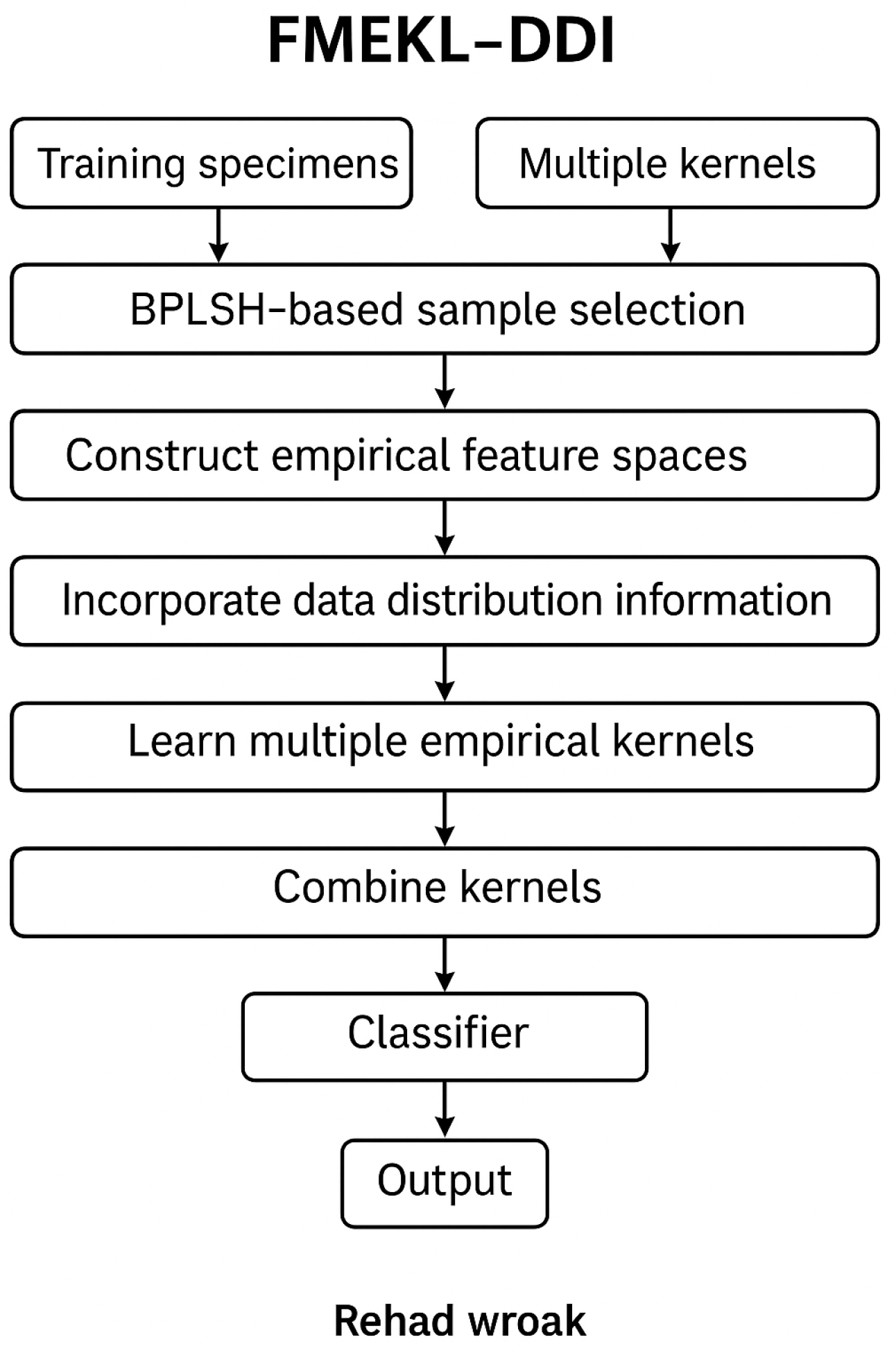
Despite its effectiveness, MEKL suffers from high computational demands due to the need to construct multiple empirical feature spaces, limiting its scalability to large datasets. To address this, researchers have explored ways to reduce training time. For instance, Fan [19] proposed the Multiple Random Empirical Kernel Learning Machine (MREKLM), which applies random projection techniques [20] to reduce computational cost by building empirical kernels using only a randomly selected subset of the data. However, MREKLM does not consider the distribution of samples, which can lead to suboptimal feature representations and decreased accuracy. To overcome these limitations, this study introduces Fast Multiple Empirical Kernel Learning Incorporating Data Distribution Information (FMEKL-DDI), which enhances empirical kernel construction by incorporating within-class distribution data. Additionally, to further reduce the sample selection time, FMEKL-DDI employs a boundary-aware sample selection strategy using the BPLSH algorithm [21], allowing the efficient identification of informative samples near decision boundaries. Together, these improvements result in faster training and more discriminative feature spaces, making FMEKL-DDI suitable for large-scale learning tasks.

To simplify the distinctions among the related models, Multiple Empirical Kernel Learning (MEKL) builds several feature spaces from the data to improve classification, but it is computationally intensive. Multiple Random Empirical Kernel Learning Machine (MREKLM) improves speeds by randomly selecting a small set of samples to create those spaces, although it ignores the distribution of data, which can hurt accuracy. Our proposed method, Fast Multiple Empirical Kernel Learning with Data Distribution Information (FMEKL-DDI), addresses this by selecting samples more intelligently—using the BPLSH algorithm—and by considering how data points are spread within each class. This allows it to strike a better balance between accuracy and efficiency.

The main contributions of this work are summarized as follows:

• We propose FMEKL-DDI, a novel empirical kernel learning method that integrates within-class distribution information through the use of the within-class scatter matrix, enhancing the quality of the empirical feature space.
• We introduce an efficient boundary-preserving sample selection mechanism based on the BPLSH algorithm, which effectively identifies informative training samples while reducing redundancy and computational overhead.
• Extensive experiments on benchmark and real-world datasets demonstrate that MEKL-DDI achieves superior accuracy and significantly lower training time compared to several state-of-the-art kernel learning approaches.

The remainder of this paper is organized as follows. Section 2 provides a review of related work, including implicit kernel mapping and the MREKLM algorithm. Section 3 presents the proposed FMEKL-DDI algorithm, detailing the incorporation of data distribution information and the construction of the classifier. Section 4 discusses the experimental setup; evaluates the performance of the proposed method through various experiments; and includes comparisons, ablation studies, and real-world dataset validations. Finally, Section 5 concludes the paper and outlines future directions for this research.

2. Related Work and Preliminaries

Kernel learning has emerged as a fundamental technique in machine learning, enabling algorithms to handle non-linear data by implicitly mapping inputs into high-dimensional feature spaces through kernel functions. Traditional methods such as Support Vector Machines and Kernel Principal Component Analysis leverage fixed kernels, but their performance is highly sensitive to kernel choice [22]. To address this, multiple kernel learning frameworks were developed, combining several base kernels to improve flexibility and adaptability to complex data structures. Over time, variants such as nonlinear MKL, data-dependent MKL, and empirical kernel learning have evolved to enhance expressiveness, efficiency, and generalization [23]. Recent advances have focused on improving computational scalability and incorporating data distribution awareness, laying the groundwork for more robust and adaptive kernel-based models [24,25].

2.1. Implicit Kernell Mapping

This section introduces implicit kernels, expressed through the inner product form of a mapping function, in contrast to the direct computational expression of empirical kernels. Implicit kernels are primarily designed for nonlinear classifiers, in contrast to linear classifiers.

Let ${\left\{(x_i,y_i)\right\}}_{i=1}^N$ denote the training dataset, where $x_i\in {\mathbb{R}}^D$ is the i-th input sample and $y_i\in \{1,\cdots ,C\}$ is its corresponding class label. Let P denote the number of selected samples via the BPLSH algorithm for constructing the empirical feature space. The kernel function is denoted by $k(x_i,x_j)$, and the kernel matrix is $K\in {\mathbb{R}}^{P\times P}$ with entries $K_{ij}=k(x_i,x_j)$. The empirical kernel mapping is represented as $\phi \left(x\right):{\mathbb{R}}^D\to {\mathbb{R}}^r$, where r is the reduced dimensionality after eigen-decomposition. The within-class scatter matrix is defined as $S_w={\sum }_{c=1}^C{\sum }_{x_i\in {\mathcal{X}}_c}(x_i-{\mu }_c){(x_i-{\mu }_c)}^T$, where ${\mu }_c$ is the mean of class c and ${\mathcal{X}}_c$ is the set of samples in class c. The weight matrix $W\in {\mathbb{R}}^{P\times P}$ has entries $W_{ij}={\displaystyle \frac{1}{N_c}}$ if $x_i$ and $x_j$ belong to the same class c; otherwise, it has 0. The diagonal matrix D has entries $D_{ii}={\sum }_{j=1}^P{W}_{ij}$. The classifier is a linear combination of mapped kernels $f\left(x\right)={\Gamma }^{\top }{\nu }_e\left(x\right)$, where ${\nu }_e\left(x\right)={[{\phi }_1\left(x\right),\cdots ,{\phi }_M\left(x\right),1]}^T$ is the augmented empirical feature vector, and $\Gamma$ is the corresponding weight vector learned using the least-squares method. We summarize all frequently used notations in

Table 1. Summary of notations and definitions.

Symbol	Definition
N	Number of training samples
D	Dimensionality of input space
C	Number of classes
$x_i\in {\mathbb{R}}^D$	i-th input sample
$y_i\in \{1,\dots ,C\}$	Label of sample $x_i$
P	Number of selected samples via BPLSH
$k(x_i,x_j)$	Kernel function between samples $x_i$ and $x_j$
$K\in {\mathbb{R}}^{P\times P}$	Kernel matrix for selected samples
$\phi \left(x\right)$	Empirical kernel mapping function
r	Reduced dimensionality after mapping
$S_w$	Within-class scatter matrix
${\mu }_c$	Mean vector of class c
${\mathcal{X}}_c$	Set of samples in class c
W	Weight matrix (intra-class similarity)
D	Diagonal matrix where $D_{ii}={\sum }_j{W}_{ij}$
${\nu }_e\left(x\right)$	Augmented empirical feature vector
$\Gamma$	Augmented weight vector
$f\left(x\right)$	Final classifier function

.

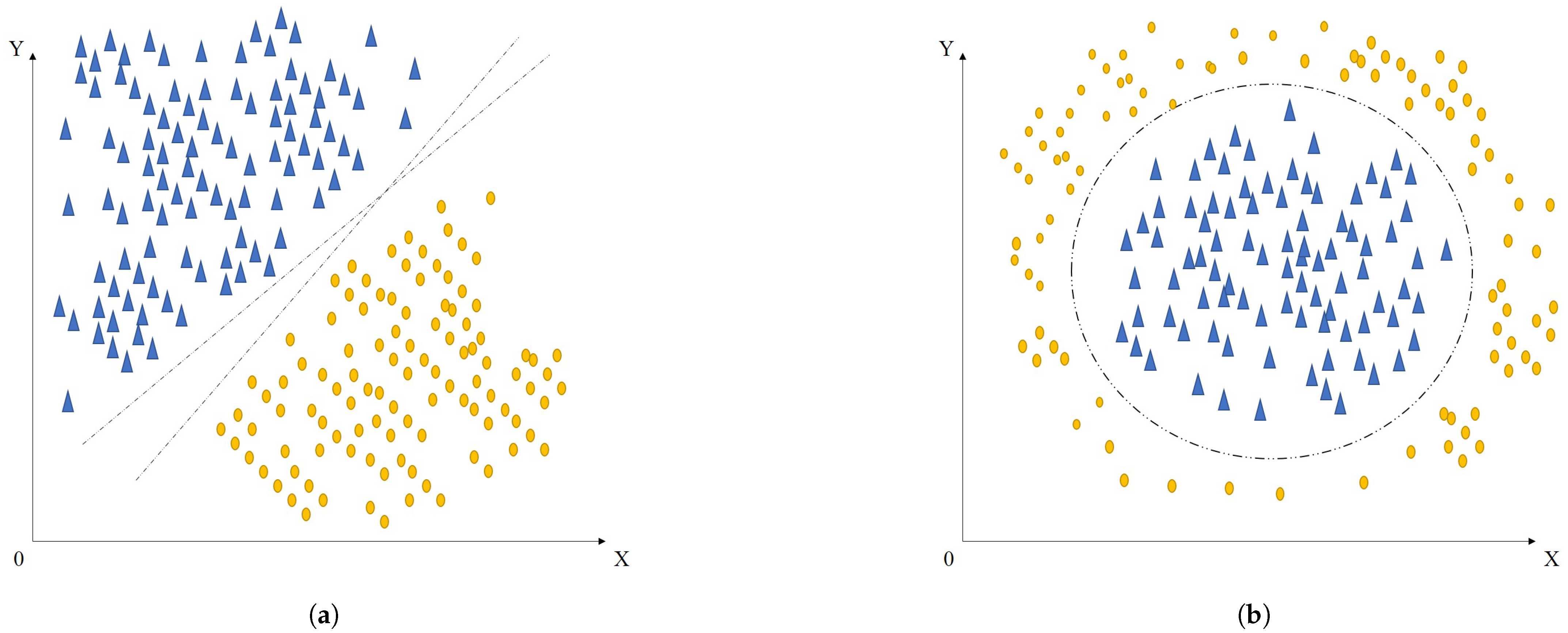
Figure 1a illustrates a scenario in which two-dimensional linearly separable samples can be effectively divided using a straight line. Consider a labeled dataset $\{(x_i,y_i)\mid i=1,\dots ,N\}$, where each label $y_i\in \{-1,+1\}$ indicates the class of the corresponding sample $x_i$. Within linear classification, a sample can be expressed as $x_i=(X_i,Y_i)$, where $X_i$ and $Y_i$ represent the horizontal and vertical coordinates, respectively. A linear decision boundary defined by the equation $w^{T}x+b=0$ can separate the two classes. The associated decision function $f\left(x\right)=w^{T}x+b$ assigns a class based on the sign of $f\left(x\right)$: if $f\left(x\right)>0$, the sample belongs to class $+1$; if $f\left(x\right)<0$, it is assigned to class $-1$; if $f\left(x\right)=0$, it lies on the decision boundary.

However, real-world data are often non-linearly separable, as shown in Figure 1b, making linear classifiers insufficient. To address this, kernel-based methods have been introduced, which use implicit mappings to transform the data into higher-dimensional spaces where linear separation becomes feasible. These methods leverage the inner product form of kernel functions. For instance, mapping a two-dimensional point $(X,Y)$ to a three-dimensional space can be carried out as $(X,Y)\to (X^2,\sqrt{2}XY,Y^2)$. This transformation can be defined by a mapping function $\varphi$. The inner product in the transformed space can be computed as follows:

$$\begin{array}{l}<\varphi \left(X,Y\right),\varphi \left(X^{\prime },Y^{\prime }\right)>=<\left(X_1,Y_1,Z_1\right),\left(X_1^{\prime },Y_1^{\prime },Z_1^{\prime }\right)>\hfill \\ =<\left(X^2,\sqrt{2}XY,Y^2\right),\left({\left(X^{\prime }\right)}^2,\sqrt{2}\left(X^{\prime }\right)\left(Y^{\prime }\right),{\left(Y^{\prime }\right)}^2\right)>\\ =X^2{\left(X^{\prime }\right)}^2+2XY\left(X^{\prime }\right)\left(Y^{\prime }\right)+Y^2{\left(Y^{\prime }\right)}^2\\ ={\left(X{X}^{\prime }+Y{Y}^{\prime }\right)}^2\\ ={(<X_N,Y_N>)}^2\\ =K(X_N,Y_N)\end{array}$$

(1)

Here, K is the kernel function, which defines an inner product in the higher-dimensional space without requiring the explicit computation of mapping $\varphi$—hence the term “implicit kernel”. This approach enables algorithms to operate in a transformed space where non-linear relationships can be addressed with linear classifiers, significantly boosting classification performance.

Nonetheless, directly applying kernel methods to certain linear discriminant analysis techniques, such as Kernel Direct Discriminant Analysis (KDDA) [26], poses challenges. Methods like Orthogonal Linear Discriminant Analysis (OLDA) [27] and Uncorrelated Linear Discriminant Analysis (ULDA) [28] rely on singular value decomposition, which complicates their kernelization. As a result, implicit kernel approaches are often employed to overcome these limitations in extending linear models to non-linear scenarios.

2.2. Multiple Random Empirical Learning Machine (MREKLM)

Fan [19] proposed the Multiple Random Empirical Kernel Learning Machine (MREKLM), which is a classic algorithm within the domain of empirical kernels. This section utilizes MREKLM as an illustrative example to introduce empirical kernels. MREKLM constructs the empirical feature space by randomly selecting a small subset of samples from the training data, and the model is presented below.

Assume the training samples $\left\{(x_i,y_i)|i=1,\dots ,N\right\}$, where $x_i\in {\mathbb{R}}^D$ and $y_i\in \left\{-1,1\right\}$. Randomly select M subsets, each of size P (where $P\le N$), that are denoted as $\left\{Su{b}_1,Su{b}_2,\dots ,Su{b}_M\right\}$ for random projection [20]. The idea is to avoid using the entire dataset to build feature spaces. Instead, smaller random subsets are used to speed up computation while still preserving meaningful structure.

For each random subset $Su{b}_m$, the corresponding random empirical kernel mapping is constructed as follows:

First, compute the kernel matrix $K_m={\left[{\left({ker}_m\right)}_{i,j}\right]}_{i,j=1}^P$, where the kernel function is defined as ${\left({ker}_m\right)}_{i,j}={\varphi }_m\left(x_m^i\right){\varphi }_m\left(x_m^j\right)$ with $x_m^i,x_m^j\in Su{b}_m$. This matrix captures the pairwise similarity between selected samples in the subset $Su{b}_m$.

The kernel matrix $K_m$ is a positive semidefinite matrix, which can be decomposed using the following:

$$K_m={\tilde{Q}}_m{\tilde{\Lambda }}_m{\tilde{Q}}_m$$

(2)

Here, ${\tilde{\Lambda }}_m$ is a $P\times P$ diagonal matrix containing the eigenvalues of $K_m$, and ${\tilde{Q}}_m$ is a $P\times P$ matrix for which its columns are the corresponding eigenvectors. This decomposition allows us to understand the underlying structure of the kernel space and reduce dimensionality while preserving variance.

The random empirical kernel mapping function ${\tilde{\varphi }}_m^e$ is defined as follows:

$${\tilde{\varphi }}_m^e\left(x\right)={\tilde{\Lambda }}_m^{-1/2}{\tilde{Q}}_m^T{\left[{ker}_1(x,x_m^1),{ker}_1(x,x_m^2),\dots ,{ker}_1(x,x_m^P)\right]}^T$$

(3)

This mapping projects a sample x into a new empirical feature space, where its coordinates are based on similarities to the reference samples in $Su{b}_m$.

It is important to note that when the rank of $K_m$ is $r_m$, it has $(P-r_m)$ zero eigenvalues. Additionally, the eigenvector matrix ${\tilde{Q}}_m$ satisfies the following:

$${\tilde{Q}}_m{\tilde{Q}}_m^T={\tilde{Q}}_m^T{\tilde{Q}}_m=I_{P\times P}$$

(4)

The eigenvalue matrix ${\tilde{\Lambda }}_m$ can be expressed as follows:

$${\tilde{\Lambda }}_m=\left[\begin{array}{ccccc}{\lambda }_m^1& & & & \\ & \ddots & & & \\ & & {\lambda }_m^{r_m}& & \\ & & & 0& \\ & & & & \ddots \end{array}\right]\in {\mathbb{R}}^{P\times P}$$

(5)

Here, ${\lambda }_m^1,\dots ,{\lambda }_m^{r_m}$ are the positive eigenvalues of $K_m$, and the zero entries correspond to redundant or non-informative directions. We discard the zero components to reduce noise and computation, keeping only the meaningful directions in the space.

After removing the zero values, we obtain an $r_m$-dimensional empirical feature vector. The reduced empirical kernel is then denoted by ${\varphi }_m^e$, and the mapping is as follows:

$${\varphi }_m^e\left(x\right)={\Lambda }_m^{-1/2}{Q}_m^T{\left[{ker}_1(x,x_m^1),{ker}_1(x,x_m^2),\dots ,{ker}_1(x,x_m^P)\right]}^T$$

(6)

Here, ${\Lambda }_m\in {\mathbb{R}}^{r_m\times r_m}$ contains positive eigenvalues, and $Q_m$ is a $P\times r_m$ matrix of the corresponding eigenvectors.

In essence, ${\varphi }_m^e\left(x\right)$ provides a compact, meaningful representation of x in the empirical feature space built from subset $Su{b}_m$.

After constructing the M empirical kernels, all training samples are mapped into each of the M empirical feature spaces. The final transformed dataset is represented as ${\left\{{\varphi }_1^e\left(x_i\right),\dots ,{\varphi }_M^e\left(x_i\right)\right\}}_{i=1}^N$. This gives us M different views of the data, each built from a random subset, which collectively capture diverse structural aspects of the dataset. These mapped features can then be used for efficient and robust classification.

3. Fast Multiple Empirical Kernel Learning Incorporating Data Distribution Information (FMEKL-DDI)

3.1. Model

MREKLM shows that creating an empirical feature space with a limited sample subset can significantly decrease training duration while maintaining training accuracy. Nonetheless, it demonstrates significant unpredictability and neglects to consider sample distribution data. This section introduces a technique called Fast Multiple Empirical Kernel Learning Incorporating Data Distribution Information (FMEKL-DDI) to tackle this issue. FMEKL-DDI incorporates the within-class scatter matrix to assimilate sample distribution data. In contrast to the random projection method employed by MREKLM, FMEKL-DDI utilizes a location-sensitive hashing algorithm (BPLSH) to pick a subset of samples for the construction of the empirical feature space. We summarize the general pipeline of our proposal in Figure 2 and Algorithm 1.

BPLSH selects a sample as the reference instance and computes the similarity index of the remaining samples [21]. If the neighboring samples of the selected instance belong to the same class and exhibit a high similarity index, those neighboring samples are discarded. If the neighboring samples belong to different classes but exhibit a high similarity index and are proximate in spatial distance, the neighboring samples are retained. If the neighboring samples of the selected instance are from different classes, exhibit a high similarity index, and are widely spaced, then the neighboring samples of the same class are discarded while preserving those from different classes. Samples with a low similarity index are not subjected to further processing. This process is iterated until all samples have been evaluated. BPLSH maintains the instance boundaries while effectively reducing the dataset in this manner.

Initially, BPLSH was designed to reduce the number of samples used for training Support Vector Machine (SVM) classifiers [29] to minimize training time. However, in the context of empirical kernels, it is employed to select samples for constructing the projection space. Following the application of the BPLSH algorithm to select samples for constructing the empirical feature space, the empirical kernel is reconstructed as follows:

$${\phi }^e\left(x_i\right)={\left(X_{\phi }^T{S}_w{X}_{\phi }\right)}^{-1/2}[k(x_i,x_1)\cdots k(x_i,x_P)]$$

(7)

This equation transforms a sample $x_i$ into the empirical kernel space while also normalizing the projection using class distribution information encoded in $S_w$.

In this context, let X be defined as the set $X_{\phi }=\left[\varphi \left(x_1\right)\cdots \varphi \left(x_P\right)\right]$. The samples designated as P are chosen through the BPLSH algorithm, and $S_w$ represents the within-class scatter matrix for these samples. $S_w$ represents the distribution of samples within each class, and the prior expression can be understood as maintaining this distributional information during projection into the empirical kernel space. The computation of $S_w$ is as follows:

$$S_w=\sum _{i\in N}{S}_i$$

(8)

Here, $S_i$ denotes the covariance matrix, with i representing the i-th class, and $S_i$ is defined as follows:

$$S_i=\sum _{x\in X_i}(x-m_i){(x-m_i)}^T$$

(9)

This matrix $S_i$ describes how data in class i are spread around its mean $m_i$. By summing across all classes, $S_w$ captures the overall within-class variation.

$m_i$ denotes the mean vector of the i-th class, where $m_i={\displaystyle \frac{1}{N^{\left(s\right)}}}{\displaystyle \sum _{i\in N^{\left(s\right)}}}\varphi \left(x_i\right)$. In Equation (7), X represents a matrix that includes the newly computed dimensional vectors for each sample, and it is derived from the kernel mapping function. For computational efficiency, $S_w$ may be reformulated as follows:

$$S_w=X_{\phi }(D-W){\left(X_{\phi }\right)}^T$$

(10)

This is a matrix reformulation of $S_w$ using graph-based structures where W encodes intra-class similarities.

D is a diagonal matrix defined by $D_{i,i}={\displaystyle \sum _{j=1}^N}{W}_{i,j}$, where W represents a weight matrix. If $y_i=y_j=s$, where s denotes the s-th class, then $W_{ij}={\displaystyle \frac{1}{N^{\left(s\right)}}}$; otherwise, $W_{ij}=0$, and an alternative form of the empirical kernel presented in this paper can then be obtained as follows:

$${\phi }^e\left(x_i\right)={\left(KLK\right)}^{-1/2}[k(x_i,x_1)\cdots k(x_i,x_P)]$$

(11)

This expression simplifies the computation while retaining the class distribution structure via matrix $L=D-W$, often called the graph Laplacian.

3.2. Classifier

This section introduces a classifier developed from the empirical kernel of FMEKL-DDI, following the formulation outlined in Equation (11). The initial step involves a training dataset represented as $\left\{(x_i,y_i)|i=1,\dots ,N\right\}$, where $y_i\in \left\{-1,+1\right\}$. The collection ${\left\{{\phi }_1^e\left(x_i\right),\dots ,{\phi }_M^e\left(x_i\right)\right\}}_{i=1}^N$ represents the transformed samples within M empirical feature spaces produced by the empirical kernel. Each ${\phi }_l^e\left(x_i\right)$ gives a different view of the same data point in its corresponding feature space, enriching the feature representation.

Upon the completion of the construction of these M feature spaces, FMEKL-DDI systematically maps P training samples into their kernel spaces. The final classifier is defined as a weighted combination of the empirical kernel feature spaces, and it is represented mathematically as follows:

$$\begin{array}{c}f\left(x\right)={\displaystyle \sum _{l=1}^M}{\lambda }_l{\Gamma }_l^T{\phi }_l^e\left(x\right)+{\Gamma }_0^T\hfill \\ ={\left(\begin{array}{c}{\lambda }_1{\Gamma }_1\\ ⋮\\ {\lambda }_M{\Gamma }_M\end{array}\right)}^T\left(\begin{array}{c}{\phi }_1^e\left(x\right)\\ ⋮\\ {\phi }_M^e\left(x\right)\end{array}\right)+{\Gamma }_0^T\hfill \\ ={\left(\begin{array}{c}{\lambda }_1{\Gamma }_1\\ ⋮\\ {\lambda }_M{\Gamma }_M\\ {\Gamma }_0\end{array}\right)}^T\left(\begin{array}{c}{\phi }_1^e\left(x\right)\\ ⋮\\ {\phi }_M^e\left(x\right)\\ 1\end{array}\right)={\Gamma }^T{\nu }^e\left(x\right)\hfill \end{array}$$

(12)

This form merges all mapped features into one augmented vector ${\nu }^e\left(x\right)$ and performs a linear classification using learned weight vector $\Gamma$.

In Equation (12), ${\lambda }_l$ indicates the weight coefficient for the l-th empirical feature space, ${\Gamma }_l$ represents the corresponding weight vector, and ${\Gamma }_0$ denotes the bias term. The augmented empirical feature vector for x is represented as ${\nu }^e\left(x\right)={\left[{\phi }_1^e\left(x\right),\dots ,{\phi }_M^e\left(x\right),1\right]}^T$, and $\Gamma$ signifies the augmented weight vector. The classifier generates probability outputs for the sample x across multiple classes. If $max\left[f\left(x\right)\right]=f_i\left(x\right)$, this indicates that the sample is classified as belonging to class i. To ascertain $\Gamma$, the minimum norm least-squares method is employed [30]. The classification information for the training samples is presented as follows:

$$t_k\left(x_i\right)=\left\{\begin{array}{cc}1,\hfill & \mathrm{if}{y}_i=k\hfill \\ 0,\hfill & \mathrm{otherwise}\hfill \end{array}\right.$$

(13)

This sets up a one-hot encoding for the true class labels, turning the classification problem into a regression task.

In this context, $t\left(x_i\right)={[t_1\left(x_i\right)\cdots t_k\left(x_i\right)]}^T$, with k denoting the total number of classes. The computation of the augmented weight vector $\Gamma$ is performed using the following method:

$$\begin{array}{c}{\Gamma }^{*}=\underset{\Gamma }{argmin}{\displaystyle \sum _{i=1}^N}\Vert {\Gamma }^T\nu \left(x_i\right)-t\left(x_i\right){\Vert }^2\hfill \\ =\underset{\Gamma }{argmin}\Vert {\Gamma }^T\nu -T{\Vert }^2\hfill \end{array}$$

(14)

We find $\Gamma$ by minimizing prediction errors over all training samples using least squares. This yields a simple and fast solution.

In this context, $\nu =[{\nu }^e\left(x_1\right),\dots ,{\nu }^e\left(x_N\right)]$ and $T=[t\left(x_1\right),\dots ,t\left(x_N\right)]$. Upon differentiating the previously mentioned expression with respect to $\Gamma$, the following results are obtained:

$${\Gamma }^{*}={\left({\nu }^T\right)}^{-1}{T}^T$$

(15)

This gives a closed-form solution to compute the optimal weights $\Gamma$ that define the final classifier.

The integration of empirically mapped samples into the classifier facilitates the generation of the final predicted classification outcomes. By combining the strengths of sample distribution awareness and fast feature construction, FMEKL-DDI achieves both efficiency and accuracy.

Algorithm 1 Fast Multiple Empirical Kernel Learning Incorporating Data Distribution Information (FMEKL-DDI)

Require: Training specimens $\left\{(x_i,y_i)\mid i=1,\dots ,N\right\}$, number of kernels M, kernel functions ${\left\{k_l(x_i,x_j)\right\}}_{l=1}^M$ Ensure: Augmented weight vector $\Gamma$ 1: Select M subspaces by choosing P samples from the training set using the BPLSH algorithm 2: for$l=1$ to M do 3:     Compute the empirical kernel mapping ${\phi }^e\left(x_i\right)$ for the l-th subspace using Equation (11) 4: end for 5: Form the augmented empirical feature vectors ${\left\{{\widehat{\phi }}_1^e\left(x_i\right),\dots ,{\widehat{\phi }}_M^e\left(x_i\right)\right\}}_{i=1}^N$ 6: Construct the target matrix T using Equation (13) 7: Compute the augmented weight vector $\Gamma$ using the least squares solution in Equation (15)

4. Experimental Results

4.1. Experimental Settings

This section will outline the parameter design of the pertinent algorithms, which will be applicable to all experiments carried out here and subsequently. All alterations to the parameters will be clearly specified in each section. This paper will also incorporate the parameter designs of more comparable algorithms, specifically FMEKL-DDI, MREKLM, MEKL, IBMPEKL [17], CGMKL [16], and NLMKL [31]. All previously stated algorithms are kernel-based, and the Gaussian kernel function $\mathrm{k}(x_i,x_j)=exp\left(-{\displaystyle \frac{{∥x_i-x_j∥}^2}{2{\sigma }^2}}\right)$ is chosen, where ${\sigma }^2=\beta ·{\displaystyle \frac{1}{N^2}}{\displaystyle \sum _{i,j\in I}}{∥x_i-x_j∥}^2$; N denotes the quantity of training samples and the kernel parameter $\beta \in \left\{{10}^{-2},{10}^{-1},{10}^0,{10}^1,{10}^2\right\}$. The quantity of kernels is selected as $M=3$. The learning rate for IBMPEKL is established at 0.99, whereas for CGMKL, it is established at 1. The intervals for the regularization parameters C and $\lambda$ are established as $\left\{{10}^{-2},{10}^{-1},{10}^0,{10}^1,{10}^2\right\}$. For BPLSH, the number of hash functions is designated as $q\in \left\{110,30,50,70,90,110\right\}$, and the number of hash families is specified as $m\in \left\{10,20,30,40,50,60\right\}$.

MREKLM entails the selection of $P\left(P\le N\right)$ samples, characterized by a selection ratio of $P/N$, where P signifies the number of selected samples and N indicates the total number of training samples. Experimental data in reference [19] indicate that when the ratio $P/N$ surpasses 0.5, there is no notable enhancement in accuracy, while the training duration increases substantially. Consequently, this study chooses $P/N\in \{0.01,0.03,0.05,0.07,0.09,0.1,0.2,0.3,0.4,0.5\}$. A five-fold cross-validation technique [32] is utilized to determine the optimal combinations of the specified parameters. The experimental configuration includes an i5-10300H processor working at 2.50 GHz, with 16 GB of RAM, a Windows 10 operating system, and MATLAB version R2021a. All experiments are conducted using this device. All datasets are sourced from the UCI repository [33].

In particular, the selection of key parameters such as the kernel bandwidth ${\sigma }^2$, the balancing factor $\beta$ in distributional alignment, and the number of hash functions used in BPLSH was guided by both empirical tuning and theoretical insights. The kernel bandwidth ${\sigma }^2$ was chosen based on principles from kernel density estimation, where an appropriately scaled bandwidth ensures a smooth yet discriminative kernel matrix, preventing over-smoothing or overfitting [34]. The parameter $\beta$ controls the trade-off between projection fidelity and distributional regularization; it was tuned empirically across datasets to maintain stability while capturing within-class scatter effectively. For BPLSH, the number of hash functions determines the sensitivity to local boundary structures. A moderate number of hashes ensures the accurate identification of informative boundary samples while avoiding excessive overlap or noise [35]. Together, these parameter choices reflect a balance between the theoretical guarantees of representation quality and practical performance observed in validation experiments.

All experiments were conducted on a system with an Intel Core i9 processor, 64 GB RAM, and an NVIDIA RTX 3090 GPU. The operating system was Ubuntu 22.04 LTS.

4.2. The Influence of the Number of Hash Functions and Hash Families on FMEKL-DDI

The BPLSH algorithm serves as the sample selection mechanism for the FMEKL-DDI algorithm, and it is characterized by two primary parameters: the quantity of hash functions q and the count of hash families m. This section of the experiment focuses on analyzing the impact of the two parameters of BPLSH on the FMEKL-DDI algorithm. The variable q is selected from the set $\{10,30,50,70,90,110\}$, and the variable m is chosen from the range $\{10,20,30,40,50,60\}$. The results from the experiments are detailed in

Table 2. Classification accuracy (%) of different algorithms on various datasets.

Dataset	FMEKL-DDI	NLMKL	MREKLM	MEKL	IBMPEKL	CGMKL
Iono	95	94	93	92	93	91
Heart	85	82	80	75	80	80
ILPD	73	72	72	72	72	73
CMC	56	55	53	52	55	54
Bupa	63	62	61	60	61	62
Magic	85	84	84	73	78	75
Twonorm	100	99	98	98	99	97
Optidigits	99	97	96	95	96	94
Coil-2000	94	93	92	91	92	90
Wdbc	97	96	95	94	96	95
Wpbc	82	80	78	76	79	81
Iris	100	97	96	94	96	95
Wine	97	95	94	93	95	93
Knowledge	95	94	91	89	93	90
EEG	96	95	95	94	95	94
Letter	100	99	99	98	99	98
Pendigits	98	97	96	95	97	95
Polish	95	94	93	91	93	92

and

Table 3. Experimental results on the Twonorm dataset.

$q=10$			$q=30$
m	Accuracy	Time (s)	m	Accuracy	Time (s)
10	0.9748	9.1898	10	0.9739	8.0213
20	0.9751	8.8932	20	0.9738	9.3807
30	0.9744	8.0264	30	0.9746	8.2321
40	0.9753	10.3214	40	0.9749	7.3459
50	0.9749	7.3458	50	0.9755	6.1234
60	0.9763	6.3841	60	0.9755	6.1245
$q=50$			$q=70$
m	Accuracy	Time (s)	m	Accuracy	Time (s)
10	0.9716	9.3524	10	0.9753	9.2134
20	0.9747	8.2359	20	0.9748	9.8921
30	0.9753	5.3524	30	0.9750	6.5987
40	0.9754	6.1945	40	0.9749	8.1945
50	0.9741	7.4682	50	0.9745	6.1503
60	0.9743	5.1564	60	0.9743	6.1324
$q=90$			$q=110$
m	Accuracy	Time (s)	m	Accuracy	Time (s)
10	0.9748	8.0421	10	0.9758	5.3424
20	0.9748	8.4245	20	0.9738	8.8320
30	0.9754	9.5623	30	0.9752	7.5362
40	0.9773	4.3421	40	0.9763	5.4215
50	0.9751	5.8742	50	-	-
60	-	-	60	-	-

. In particular, the authors of [36] demonstrate that training two-layer neural networks exhibits sharp phase transitions in generalization performance based on mini-batch size, with learning failing below a critical threshold and succeeding above it.

The results of the experiments indicate that the number of hash functions and hash families does not significantly impact the training time. It can be concluded that as long as these parameters fall within a certain range, they do not adversely affect the experimental results.

Nevertheless, this experiment faced occurrences where certain settings did not produce results. Table 2 and Table 3 illustrate that when the number of hash families is 110 and the number of hash functions is 50 or more, no pertinent experimental findings were produced, suggesting a software anomaly. Upon excluding program-related difficulties, it was concluded that the categorization inconsistencies stemmed from an inadequate number of samples chosen in the final stage. Moreover, the consistently strong performance of FMEKL-DDI is largely due to its ability to align with the underlying data distribution through the within-class scatter matrix and its focus on boundary sample selection via BPLSH, which enhances class separation. These mechanisms enable the better adaptation of kernel learning relative to both linear and non-linear class structures. The variations in performance across datasets can be explained by how well each algorithm captures critical decision boundaries—FMEKL-DDI performs especially well when boundary samples and distribution alignment significantly impact classification, whereas other methods that rely on random or uniform sampling tend to underperform in such cases.

In conclusion, the performance of the FMEKL-DDI algorithm is significantly affected by the parameters m and q. On both the Iono and Twonorm datasets, higher values of m typically sustain high accuracy; however, in some instances, excessively high values of q can result in reductions in accuracy and increases in computational time. Therefore, the ranges $10\le q\le 70$ and $10\le m\le 40$ are regarded as appropriate.

4.3. Training Time Comparison

This segment of the experiment examines the efficacy of the FMEKL-DDI algorithm in relation to training duration. The comparable algorithms still under consideration in the experiment are NLMKL, MREKLM, MEKL, IBMPEKL, and CGMEKL. Furthermore, prior studies have demonstrated that the quantities of hash functions and hash families for FMEKL-DDI need not be excessive; hence, we established (q = 30) and (m = 20) for this investigation. This section includes eighteen datasets: Wdbc, Wpbc, Iris, Wine, Knowledge, EEG, Letter, Pendigits, and Polish; all were obtained from the UCI repository. Of these, ten datasets are classified as small-scale, whilst eight are designated as relatively larger datasets, with comprehensive details presented in

Table 4. The training datasets.

Data	Attribute	Class	Instance
Iono	34	2	351
Heart	13	5	303
ILPD	10	2	583
CMC	9	3	1473
Bupa	6	2	345
Magic	10	2	19,020
Twonrom	20	2	7400
Optidigits	64	10	5620
Coil-2000	85	2	9822
Wdbc	30	2	569
Wpbc	33	2	198
Iris	4	3	150
Wine	14	2	178
Knowledge	5	4	403
EEG	14	2	14,980
Letter	16	26	20,000
Pendigits	16	10	10,992
Polish	64	2	10,313

. The experimental findings are presented in

Table 5. Training time(s) comparison on the datasets.

Data	FMEKL-DDI	NLMKL	MREKLM	MEKL	IBMPEKL	CGMKL
Iono	0.0021	0.0893	0.0024	0.0606	0.0931	0.0724
Heart	0.0025	0.0022	0.0050	0.0356	0.0542	0.0389
ILPD	0.0014	0.6277	0.0014	0.2634	0.0265	0.0254
CMC	0.0076	6.1457	0.0096	5.1785	5.5783	6.3125
Bupa	0.0021	0.0882	0.0035	0.0793	0.1024	0.0832
Magic	15.639	2351.1546	392.4778	2241.9020	2341.3212	2298.2154
Twonorm	1.1692	1425.3651	1.8548	1057.1010	1325.1134	1195.8754
Optdigits	16.2351	834.1526	73.2354	724.5102	925.3134	917.3874
Coil-2000	2.4478	380.7324	10.7393	320.7481	290.3487	215.1548
Wdbc	0.0297	0.2310	0.0397	0.1853	0.2312	0.1465
Wpbc	0.0051	0.1109	0.0121	0.0277	0.0359	0.0298
Iris	0.0011	0.0217	0.0321	0.0045	0.0054	0.0048
Wine	0.0015	0.0216	0.0123	0.0058	0.0093	0.0065
Knowledge	0.0022	0.0722	0.0053	0.0659	0.0836	0.0724
EEG	19.953969	1431.2545	256.7029	1344.23546	1521.3458	1132.4562
Letter	16.3313	2418.2577	640.3294	2138.7124	2531.4561	2214.5387
Pendigits	7.241025	340.5572	63.9967	337.2891	350.4852	362.1486
Polish	4.0005	380.5272	74.1873	369.9875	380.1354	360.5348

. The experimental result for each dataset is the average value derived from ten experiments.

Table 5 indicates that the training duration of FMEKL-DDI has been markedly diminished relative to other algorithms. For specific small datasets, while the training duration of FMEKL-DDI is diminished, the variation is not markedly significant. Nonetheless, with comparatively bigger datasets, it is apparent that the training duration of FMEKL-DDI has markedly diminished, consequently illustrating its efficacy in terms of training time.

In particular, while methods such as MEKL and IBMPEKL can achieve competitive accuracy, they often do so at the cost of significantly longer training times due to complex kernel computations and iterative optimization procedures. Conversely, MREKLM reduces training times through random sampling but may sacrifice accuracy due to suboptimal feature space representation. FMEKL-DDI effectively balances this trade-off by leveraging distribution-aware sample selection and efficient empirical kernel construction, achieving high accuracy with minimal computational cost. Understanding and explicitly managing this trade-off is crucial, particularly in real-world applications where resources are limited and timely decision-making is critical.

4.4. Classification Accuracy Comparison

This segment of the experiment mostly evaluates the classification accuracy of FMEKL-DDI in comparison to other algorithms. The algorithm parameter settings are unchanged from the previous section, and the datasets comprise eighteen datasets obtained from the UCI repository. The algorithms evaluated alongside FMEKL-DDI comprise NLMKL, MREKLM, MEKL, IBMPEKL, and CGMEKL.

The experimental outcomes are illustrated in Table 2, with the height of the bar graph indicating the classification accuracy of each technique across various datasets; taller bars signify greater accuracy. The results indicate that FMEKL-DDI attains the highest classification accuracy when compared to the evaluated methods. Additionally, Table 2 demonstrates that FMEKL-DDI consistently outperforms in classification across all eighteen datasets, highlighting its exceptional classification effectiveness.

4.5. Ablation Experiments Conducted to Validate the Functions of the Intra-Class Variance and BPLSH Modules

FMEKL-DDI consists of two modules: Intra-Class Variance $S_w$ and BPLSH. This section seeks to assess the impact of the two modules on five datasets: Iono, Iris, CMC, Twonorm, and EEG. This validation utilizes several algorithms: the original empirical kernel (EKM), the empirical kernel enhanced with Intra-Class Variance (EKM+$S_w$), the empirical kernel integrated with BPLSH (EKM+BPLSH), and the empirical kernel that combines both Intra-Class Variance and BPLSH (EKM+$S_w$+BPLSH). The statistical data compare the training durations and classification accuracies of each algorithm across the datasets (Figure 3). Training utilizes 50% of the data, with the remaining 50% allocated for testing, and results are averaged accordingly (

Table 6. Quantitative comparison of kernel learning methods included a discussion in Section 5 on the potential use of virtual threads (e.g., Java Virtual Threads or user-level threading in C++) to enhance concurrency. We reflect on how this could improve training efficiency for large datasets by optimizing parallel processing during kernel computation and BPLSH-based selection.

Method	Avg. Accuracy (%)	Avg. Training Time (s)	Scalability	Interpretability
NLMKL	92.1	635.1	Low	Low
MREKLM	90.5	74.3	High	Moderate
MEKL	88.4	627.6	Low	Moderate
IBMPEKL	91.7	748.2	Moderate	Moderate
CGMKL	90.8	613.5	Moderate	Low
FMEKL-DDI	94.6	6.8	High (efficient with large data)	Moderate to High

). The entries highlighted in

Table 7. The accuracy (%) comparison of ablation experiments.

Data	EKM	EKM+${\mathit{S}}_{\mathit{w}}$	EKM+BPLSH	EKM+${\mathit{S}}_{\mathit{w}}$+BPLSH
Iono	92.94	95.36	92.13	95.28
Iris	97.35	99.26	96.94	99.19
CMC	54.50	56.54	54.31	56.50
Twonorm	97.87	100.00	97.46	99.98
EEG	90.73	96.50	90.41	96.36

represent the highest accuracy, whereas those in

Table 8. The comparison of training time(s) in ablation experiment.

Data	EKM	EKM+${\mathit{S}}_{\mathit{w}}$	EKM+BPLSH	EKM+${\mathit{S}}_{\mathit{w}}$+BPLSH
Iono	0.0605	0.0656	0.0031	0.0124
Iris	0.0045	0.0042	0.0011	0.0014
CMC	5.1785	4.9620	0.0730	0.0931
Twonorm	1057.1012	960.3523	1.3521	1.7532
EEG	1344.2353	1432.5832	9.5432	15.3453

signify the shortest training time. Notably, we used a 50/50 train–test split to ensure a balanced evaluation between training efficiency and generalization performance. This ratio was consistently applied to maintain comparability across experiments and to avoid bias from overly skewed training or testing proportions.

Table 7 illustrates that the integration of EKM and $S_w$ achieves the best accuracy, signifying that the inclusion of Intra-Class Variance substantially boosts the accuracy of the empirical kernel and affirming that $S_w$ contributes to accuracy improvement. The isolated introduction of BPLSH results in a little decrease in EKM accuracy, indicating that BPLSH’s effect on categorization accuracy has diminished. This signifies that inside the amalgamation of EKM+$S_w$+BPLSH, solely $S_w$ is employed to enhance accuracy.

Table 8 demonstrates that the amalgamation of BPLSH with EKM results in the minimal training time, indicating that BPLSH significantly decreases training duration. Conversely, employing only the empirical kernel with $S_w$ leads to a slight extension of training time, indicating that $S_w$ does not contribute to reducing training duration. Utilizing both $S_w$ and BPLSH yields favorable outcomes in classification accuracy and training duration for the empirical kernel.

The training time differences among the compared algorithms primarily stem from the sample selection and kernel evaluation strategies. FMEKL-DDI achieves superior efficiency by leveraging the BPLSH algorithm to intelligently select a smaller, boundary-representative subset of samples, significantly reducing unnecessary computations. Additionally, the use of reduced kernel evaluations in smaller, well-structured empirical feature spaces contributes to faster processing. In contrast, while MREKLM also reduces training time by using random subsets, it occasionally incurs higher overhead due to the unpredictability of random sampling, which may select less informative or redundant data, requiring more iterations or larger projections to achieve acceptable performance.

4.6. Experiments on the Protein Subcellular Localization Dataset

To further validate the practicality and generalizability of the proposed algorithm, this section selects three datasets focused on protein subcellular localization to evaluate its performance. The three datasets analyzed are Plant, PsortPos, and PsortNeg. The Plant dataset consists of four classes and a total of 940 samples; PsortPos includes four classes with 541 samples, while PsortNeg comprises five classes with 1441 samples. Fifty percent of the data is utilized for training, while the remaining fifty percent is reserved for testing.

As illustrated in Figure 4, it is evident that FMEKL-DDI demonstrates strong performance in practical applications. Notably, FMEKL-DDI achieves the highest classification accuracy, consistent with the results obtained in previous experimental sections. Furthermore, the classification accuracy of FMEKL-DDI is markedly higher than that of the other algorithms.

5. Conclusions

This paper proposed an efficient algorithm—Fast Multiple Empirical Kernel Learning Incorporating Data Distribution Information (FMEKL-DDI)—that integrates within-class distribution characteristics and boundary-aware sample selection to improve classification performance and computational efficiency. The experimental results across 18 benchmark datasets and 3 protein subcellular localization datasets demonstrated that FMEKL-DDI consistently outperformed comparable methods in terms of both classification accuracy and training time. Our proposal is well suited for large-scale, high-dimensional tasks where accuracy and efficiency are critical. It is particularly useful in bioinformatics, medical diagnostics, and security applications—such as protein classification, disease detection, and fraud or intrusion detection—where preserving class boundaries and fast model training are essential for real-time decision-making.

The observed improvements are largely attributed to two main components of the method: (1) the use of the within-class scatter matrix ($S_w$), which enables the model to preserve class-specific sample distributions in the empirical kernel space, and (2) the application of the BPLSH algorithm, which selects informative border samples while significantly reducing the size of the training set. This combination allows FMEKL-DDI to strike an effective balance between accuracy and efficiency, especially on large-scale and high-dimensional datasets.

Comparative analysis showed that FMEKL-DDI surpasses state-of-the-art algorithms such as MEKL, MREKLM, IBMPEKL, CGMKL, and NLMKL in both predictive power and computational scalability. While some baseline methods achieved acceptable accuracy, they often incurred higher computational costs. In contrast, FMEKL-DDI maintained competitive accuracy with substantially lower training times, making it more practical for real-world applications.

An interesting direction for enhancing the training efficiency of FMEKL-DDI, especially on large-scale datasets, lies in leveraging virtual threads—such as Java Virtual Threads or user-level threading in C++. These lightweight threads offer low-overhead concurrency, enabling fine-grained parallelism during computationally intensive tasks like kernel matrix construction and BPLSH-based boundary sample selection. By parallelizing kernel evaluations across multiple subspaces or concurrently processing similarity computations in BPLSH, the algorithm could significantly reduce wall-clock training time without increasing memory consumption. Integrating virtual threads into the existing framework would allow the more efficient utilization of multi-core architectures, making FMEKL-DDI even more scalable for high-dimensional or streaming data applications.

Despite these advances, several opportunities for future development remain. One area involves exploring adaptive strategies for selecting the number and type of empirical kernels based on dataset characteristics. Another promising direction is the integration of class imbalance handling techniques and robust noise filtering, which could further enhance model generalization in complex or imbalanced datasets. Additionally, extending FMEKL-DDI to semi-supervised or online learning scenarios would broaden its applicability in dynamic and data-scarce environments.