Article

A Two-Stage Fault Reconfiguration Strategy for Distribution Networks with High Penetration of Distributed Generators

1
Hangzhou Power Supply Company, State Grid Zhejiang Electric Power Co., Ltd., Hangzhou 310016, China
2
College of Electrical Engineering, Zhejiang University, Hangzhou 310027, China
*
Author to whom correspondence should be addressed.
Electronics 2025, 14(9), 1872; https://doi.org/10.3390/electronics14091872
Submission received: 18 March 2025 / Revised: 28 April 2025 / Accepted: 30 April 2025 / Published: 4 May 2025
(This article belongs to the Special Issue Power Electronics in Renewable Systems)

Abstract

In distribution networks with high penetration of distributed generators (DGs), traditional fault reconfiguration strategies often fail to achieve maximum load recovery and encounter operational stability challenges. This paper proposes a novel two-stage fault reconfiguration strategy that addresses both the fault ride-through capability and output uncertainty of DGs. The first stage introduces a rapid power restoration reconfiguration model that integrates network reconfiguration with fault ride-through, enabling DGs to provide power support to the distribution network during faults, thereby significantly improving the recovery rate of lost loads. An AdaBoost-enhanced decision tree algorithm is utilized to accelerate the computational process. The second stage proposes a post-recovery optimal reconfiguration model that uses fuzzy mathematics theory and the transformation of chance constraints to quantify the uncertainty of both generation and load, thereby improving the system’s static voltage stability index. Case studies using the IEEE 69-bus system and a real-world distribution network validate the effectiveness of the proposed strategy. This two-stage strategy facilitates short-term rapid load power restoration and enhances long-term operational stability, improving both the resilience and reliability of distribution networks with high DG penetration. The findings of this research contribute to enhancing the fault tolerance and operational efficiency of modern power systems, which is essential for integrating higher levels of renewable energy.

1. Introduction

The primary task of a distribution network is to deliver electricity to end-users. As society progresses, users’ demands for the quality and reliability of power supply have been steadily increasing. Distributed generators (DGs) provide a broader range of energy sources for distribution networks. However, as the penetration level of DGs increases, maintaining smooth and uninterrupted operation of distribution networks presents significant challenges. Renewable energy devices typically lack the rotational inertia inherent to conventional thermal power units, resulting in a weakened frequency regulation capability of the grid. To address frequency stability issues, grid-forming inverter technologies, such as virtual synchronous generators, virtual impedance control, virtual inertia control, and virtual oscillator control, have been developed [1,2,3].
The power output of distributed renewable energy sources is inherently volatile, which may lead to local voltage rises or sags, resulting in voltage violations. To mitigate these effects, DGs can be effectively coordinated with other flexibility resources across multiple time scales through mechanisms such as virtual power plants (VPPs) and microgrids [4,5]. This coordination enables aggregated resources to participate as a unified entity in electricity market operations, facilitating optimized dispatch. Furthermore, by deploying energy storage systems, fluctuations in distributed generation output can be smoothed, thereby achieving better power matching between generation and load [6]. In distribution networks with high DG penetration, bidirectional power flows become common, rendering traditional grid protection schemes insufficient. Adaptive protection schemes or novel intelligent algorithms need to be developed to address these new protection challenges [7]. Islanded microgrid technologies offer a promising solution by enabling parts of the distribution system to operate independently from the main grid following a fault [8].
In addition, fault reconfiguration serves as an essential means to ensure supply reliability and maintain smooth, uninterrupted operation of the system. Fault reconfiguration technology refers to an optimization technique whereby, upon a fault occurring in the distribution network, the system’s topology is modified to transfer the lost load in non-faulted areas to other feeders or generators that still have power supply capability, enabling rapid restoration of power supply [9].
The integration of a substantial number of DGs into distribution networks has introduced significant challenges to the fault reconfiguration process [10,11]. On one hand, DGs have transformed the distribution network from a traditional single-source structure to a multi-source structure, providing more flexible and diverse recovery options in case of faults. DGs with frequency regulation and voltage stabilization capabilities can support islanded operation of the distribution network during faults, while DGs with fault ride-through capabilities can forcibly remain connected to the grid for a short period to support system power balance [12,13]. On the other hand, the multi-source structure complicates fault reconfiguration, requiring consideration of factors such as power output characteristics and topological constraints. Moreover, the uncertainty of DG output necessitates dynamic adjustments to fault reconfiguration strategies [14].
The issue of fault reconfiguration for distribution networks with DGs has been extensively addressed in the existing literature, with the primary focus on fault ride-through (FRT) characteristics during fault events and the impacts of post-fault uncertainty. In [15], the authors investigate the relationship between fault ride-through characteristics of DGs and their power recovery support capabilities, proposing a multi-stage self-healing method based on the margin capacity of interconnection lines. In [16], the authors analyze the electrical output characteristics of inverter-based DGs during both normal operation and fault ride-through conditions. In [17], the authors propose a fault reconfiguration scheme for distribution networks that coordinates reclosing operations with DGs’ LVRT capabilities. However, these studies have primarily focused on analyzing the impact of DGs’ fault ride-through characteristics on fault reconfiguration, while offering limited incorporation of this condition within the reconfiguration algorithms themselves.
In [18], the authors emphasize that to ensure the long-term stability of distribution networks, fault reconfiguration strategies must account for dynamic variations in generation and load over multiple time periods. In [19], the authors use C-Vine Copula and conditional probability to characterize the dynamic uncertainty of renewable energy sources. In [20], the authors analyze the impact of the stochastic nature of renewable energy output on system stability, and propose a fault reconfiguration algorithm based on probabilistic power flow. In [21], a fault recovery model based on robust stochastic optimization is proposed to address the uncertainty of DG output. However, the methods still exhibit the following issues: they rarely account for the uncertainties associated with the output of DGs and load power, leading to lower reliability; and they primarily focus on load shedding and switch operation counts, with less consideration given to the impact on system stability. Additionally, the stability indicators for distribution networks are often nonlinear, making them difficult to handle [22].
In the absence of sufficient operational data and accurate forecasting methods, fuzzy mathematical theory provides an effective approach for analyzing uncertainty, and offers greater applicability in practical scenarios [23,24]. In [25], the authors investigate energy management in multi-energy microgrids using an optimization algorithm integrated with fuzzy decision-making techniques, demonstrating the effectiveness of fuzzy methods in handling uncertain conditions in complex energy systems. In [26], the authors propose a two-stage robust adaptive model, based on a predictive control approach, for the optimal scheduling of integrated energy systems, incorporating fuzzy-inspired uncertainty modeling and adaptive control to balance economy and robustness.
The fault ride-through capability and output uncertainty of DGs exhibit differences in time scales. During the fault recovery process, fault ride-through plays a role in the early stages of the fault, while output uncertainty affects the system’s operation after the fault. Few studies simultaneously consider the impacts of both factors and achieve the dual objectives of rapid power restoration and long-term operational stability. Furthermore, due to the inclusion of fault ride-through control and output uncertainty of DGs, fault reconfiguration models tend to be nonlinear and complex. Traditional solution methods may suffer from slow computational speed [27], which makes them less suitable for fast power restoration requirements. To address this, heuristic algorithms, such as decision trees [28] and genetic algorithms [29], are often used to enhance solution speed. Nevertheless, these methods still face challenges, such as the risk of converging to local optima in complex scenarios and the requirements of high quality for training data.
To address the issues outlined above, this paper proposes a two-stage fault reconfiguration strategy that comprehensively considers both the fault ride-through capability and the output uncertainty of DGs, aiming to improve both the short-term power restoration performance and the long-term operational stability of the distribution network system. Specifically, the contributions of this paper are as follows:
  • Establishing a rapid power restoration reconfiguration model, in which different handling strategies are applied to various types of DGs during fault recovery by adding specific constraint conditions, handled based on the Big-M method, that account for the fault ride-through, improving the load recovery percentage for areas that have lost power supply;
  • Proposing a fast solution algorithm for the reconfiguration model based on an AdaBoost-enhanced decision tree, which accelerates the solving process while maintaining the same accuracy;
  • Establishing a post-recovery optimal reconfiguration model by assessing system stability using a linearized static voltage stability index, modeling the uncertainty of DG output and load power based on fuzzy mathematics theory, and applying fuzzy chance constraint transformation to facilitate the model’s solution.
The main contents of the subsequent sections are as follows: Section 2 analyzes the role of DGs in distribution network fault recovery, including a classification-based treatment strategy for DGs, which considers fault ride-through capabilities and analysis of uncertainty and stochastic processes, and presents a two-stage fault reconfiguration strategy. Section 3 proposes a rapid power restoration strategy and introduces a fast solution algorithm based on AdaBoost-enhanced decision trees. Section 4 establishes a post-recovery optimal reconfiguration model, incorporating fuzzy representations of uncertainties and the transformation of fuzzy chance constraints. Section 5 conducts case studies using the IEEE standard system and a real-world distribution network example, comparing multiple algorithms to validate the effectiveness of the proposed approach. Finally, Section 6 concludes the paper.

2. The Impacts of DGs on Distribution Network Fault Recovery

2.1. Analysis of the Support Capability of DGs

2.1.1. Fault Ride-Through Characteristics of DGs

Considering the safety and stability of active distribution networks, DGs should have low-voltage ride-through (LVRT) capability [30]. IEEE 1547-2018 [31] establishes relevant requirements for the fault ride-through capability of DGs, classifying them into three response categories. DGs should have LVRT capability, meaning that when grid disturbances or faults cause voltage drops at the point of common coupling (PCC), DGs should continue to operate without disconnecting from the grid for a specified duration. This helps to prevent cascading failures that could lead to widespread power outages. The requirements for the LVRT capability of DGs are shown in Figure 1.
In the normal operation region (UDG ≥ 0.9 p.u.), the DG remains in a grid-connected state. When the voltage drop is relatively minor (0.2 p.u. ≤ UDG ≤ 0.9 p.u.), the DG continues to operate without disconnecting from the grid, with an output power not less than 80% of that before the disturbance or fault occurred. When the voltage drop point is severe (UDG ≤ 0.2 p.u), the DG is disconnected from the system.
During the fault recovery process, the status of the DG may vary with voltage and frequency fluctuations at the PCC. Considering the limitations in the data processing capabilities of equipment and the real-time requirements for generating power restoration schemes, it is necessary to simplify the calculation of the DG’s support capacity for engineering purposes.
When a fault causes a voltage drop at UDG, the total output current may exceed the maximum allowable short-circuit current due to the control strategy. To ensure device safety, the DG output power is subject to the following constraint:
P DG 2 + Q DG 2 I max 2 U DG 2 , U DG > 0.2   p . u . P DG = 0   ,   Q DG = 0 , U DG 0.2   p . u .
where PDG is the active power of the DG; QDG is the reactive power of DG. Imax is typically 1.2 to 2 times the rated current [32].

2.1.2. Handling Strategies for Different Types of DGs During Fault Recovery

Currently, inverter-based DGs, such as wind and solar DGs, can be categorized into grid-following and grid-forming types based on their grid connection control methods. Both grid-forming DGs and grid-following DGs with fault ride-through capabilities can provide active support to the system during fault recovery. Therefore, different handling strategies should be considered for different types of DGs.
(1)
Directly decommissioned type
After fault isolation, if there is no grid-forming DG within the downstream area of the fault point to provide frequency or voltage support, DGs without fault ride-through capability should be decommissioned.
(2)
Fault ride-through type
After a fault occurs, grid-forming DGs and grid-following DGs with fault ride-through capabilities begin fault ride-through. If the voltage meets the requirements, the DGs remain connected to the grid; otherwise, they are disconnected.

2.2. Analysis of the Output Uncertainty of DGs

For a distribution system that has just recovered from a fault and is in a relatively fragile state, the uncertainty in both power supply (from DGs) and load demand can exacerbate system instability, posing significant risks. The calculation based on the state of the system at the time of the fault will lead to neglect of the potential power change of the generation and load, and this prediction error will make the reconfiguration result no longer effective. After fault isolation and partial restoration, it is essential to readjust the distribution network to adapt to subsequent operational requirements and enhance its long-term operational capability.
The power output of DGs during a fault recovery period can be predicted using various forecasting methods. However, due to measurement errors during data collection, as well as the inherent limitations of predictive models in addressing complex scenarios, significant deviations may arise between the actual power output of the DG and its predicted value. This deviation can be expressed as follows:
P ˜ DG t = P ¯ DG t + Δ DG t
where P ˜ DG t is the actual power value of the DG at time t; P ¯ DG t is the predicted power value of the DG at time t; and Δ DG t denotes the deviation between the actual value and the predicted value of the DG.
The deviation between the predicted and actual output values of DGs is commonly described using probability distribution functions. The probability distribution functions for the output deviation of various types of DGs are as follows:
(1)
Photovoltaic generation
The probability distribution function for the deviation between the predicted and actual output of a photovoltaic generator can be described by the TLS (t location-scale) distribution, as expressed mathematically below:
ϕ ( P ˜ pv t ) = Γ ( v + 1 2 ) σ pv v π Γ ( ν 2 ) ν + ( P ˜ pv t P ¯ pv t σ pv ) 2 v v + 1 2
where P ˜ pv t and P ¯ pv t represent the actual and predicted power values of the photovoltaic system at time t, respectively; σpv and ν are the parameters for the probability distribution of the photovoltaic output deviation; and Γ is the Gamma function.
(2)
Wind turbine generation
The probability distribution function for the deviation between the predicted and actual output of a wind turbine generator can be described by the Weibull distribution, with the following mathematical expression:
P ¯ wind t = 0 , v wind t v wind , ci a + b v wind t , v wind , ci v wind t v wind , e P wind , e , v wind , e v wind t v wind , co
a = P wind , e v wind , ci v wind , ci v wind , e , b = P wind , e v wind , e v wind , ci
ϕ ( P ˜ wind t ) = K C P ¯ wind t a b C K 1 exp P ¯ wind t a b C K
where P ˜ wind t and P ¯ wind t are the actual and predicted power values of the wind turbine at time t, respectively; v wind t is the wind speed at time t; νwind,ci, νwind,co, and νwind,e are the cut-in, cut-out, and rated wind speeds of the wind turbine, respectively; Pwind,e is the rated output power of the wind turbine; K is the shape parameter of the Weibull distribution; and C is the scale parameter.
(3)
Conventional DGs
Conventional DGs, such as gas turbines and diesel generators, generally produce stable power output when the fuel supply is sufficient. The power output deviations of such systems are often modeled using a discrete 0–1 probability distribution. In this model, the generator is assumed to either be in normal operation, producing the scheduled power output, or shut down, producing no power. The mathematical expression for this is as follows:
P ( P ˜ DG , c t = P ¯ DG , c t ) = p normal
where P ˜ DG , c t and P ¯ DG , c t are the actual and scheduled power values of the conventional DG at time t, respectively, and pnormal is the probability that the generator is operating normally.

2.3. Two-Stage Fault Reconfiguration Strategy for Distribution Networks with DGs

The traditional fault reconfiguration strategy does not consider the changes brought about by DG integration. Firstly, the DG’s fault ride-through capability provides additional power support. Secondly, the output uncertainty of DGs will make the restored system potentially unstable. Ignoring these factors will make the reconfiguration result unreliable. In the early stage of the fault, the primary task is to ensure the continuous power supply of important loads. After the fault is completely isolated and the system is restored to stability, the grid-connected DG can be re-connected to the system. At this point in time, the power grid can be reconfigured again to eliminate short-term overload and ensure the long-term stable operation of the system until the faulted line is repaired. It is difficult for existing methods to meet the requirements of load recovery speed and long-term stability at the same time.
The LVRT characteristics exhibit dynamic responses in a matter of seconds, while the output volatility involves longer time scales. Based on the above analysis, to maximize the support capability of DGs in the early stages of a fault and simultaneously consider the potential long-term stability impacts of their output uncertainty on the system, a staged optimization strategy must be adopted.
In response to the above problems, this paper proposes a two-stage fault reconfiguration strategy, as shown in Figure 2.
The first stage is a rapid power restoration stage, considering the LVRT capability of DGs and aiming to minimize load shedding, and involves fast optimal calculations. It makes full use of the support capacity of the DG, and provides a very fast solution speed, which can provide a rapid power supply restoration scheme.
The second stage is a post-recovery optimal reconfiguration stage, aiming to optimize system stability and minimize load shedding. It focuses on dealing with the uncertainty of DGs and loads, improving the stability of the distribution network system for a long time.

3. Rapid Power Restoration Strategy

3.1. Rapid Power Restoration Reconfiguration Model Considering FRT Capability of DGs

3.1.1. Objective Function of Rapid Power Restoration Reconfiguration Model

After a fault occurs, we assume that the fault location has already been identified, and that the faulted lines have been isolated from the network. In the rapid power restoration stage following a fault, the system’s primary objective is to restore power to the lost loads as quickly as possible by regulating tie switches and fully utilizing DGs and other devices capable of supporting the system’s power supply. Thus, the optimization strategy for this stage is focused on ensuring continuous power supply to critical loads, with the objective function formulated as follows:
F 1 = min i Ω load ϖ i ( P load , i , 0 P load , i )
In Equation (8), ϖ i is the priority of load i, where a larger value indicates higher importance of the load; Pload,i,0 is the pre-fault power of load i; Pload,i is post-fault power of load i; and Ωload is the set of loads connected to the system.

3.1.2. Constraints of Rapid Power Restoration Reconfiguration Model

The rapid power restoration reconfiguration model must satisfy the following constraints:
(1)
DG output power constraint
The constraint on the DG’s output described in Equation (1) is a piecewise function, which is handled using the Big-M method in this paper:
P DG 2 + Q DG 2 I max 2 U DG 2 M α on P DG 2 + Q DG 2 M α on α on U DG / 0.2
αon is a binary variable, where a value of 1 indicates that the DG is connected to the grid, and 0 indicates that the DG is disconnected; and M is a sufficiently large positive constant. In this paper, M was calibrated as the upper limit of the DG output power.
For DGs using a virtual impedance control strategy, they are handled by introducing the auxiliary binary variables αz1 and αz2:
Z DG = α z 1 Z 0 + α z 2 Z virtual α z 1 + α z 2 = 1 0.9 α z 1 + 0.2 α z 2 U DG α z 1 + 0.9 α z 2
where ZDG is the additional impedance in series with the DG, Z0 is the impedance of the DG during normal operation, and Zvirtual is the virtual additional impedance of the DG.
(2)
Radial network constraint
The distribution network should maintain radial operation, ensuring that the reconfigured network does not form unintended islands. In this paper, a description method based on the non-connectivity condition of the power supply loop is adopted [33]. Compared to the conventional spanning tree model, this method offers a reduced scale and complexity.
l = 1 L y l = N b 1 m = 1 M h y h m M h 1 , h = 1 , 2 , ... , H
where l is the branch index of the distribution network; L is the total number of branches; Nb is the number of nodes; yl is a binary variable representing the status of the l-th branch, where 1 indicates that the branch is closed and 0 indicates that the branch is open; Mh is the number of branches in the h-th power supply loop; H is the total number of power supply loops; and yhm is a binary variable representing the status of the m-th branch in the h-th power supply loop.
(3)
Other constraints
Other constraints are provided in Appendix A, including power flow constraints using second-order cone relaxation, line operational safety constraints to prevent line overloads, voltage constraints to prevent overvoltage at nodes, and energy storage output constraints.

3.2. Fast Solution Algorithm for Rapid Power Restoration Reconfiguration Model

3.2.1. Fast Solution Algorithm Based on Decision Trees

For the power restoration model established above, conventional mathematical optimization methods may struggle to meet the real-time solution requirements. To overcome this challenge, this paper proposes a fast solution algorithm based on decision trees. This method based on decision trees has the characteristics of rapid computation speed and strong interpretability, while also exhibiting excellent adaptability to a wide range of operating conditions [34]. The workflow of the proposed method is shown in Figure 3.
The fast algorithm based on decision trees consists of two main components: the “knowledge base” and the “inference machine”. The “knowledge base” is a collection of instances, each containing the system’s operational state, fault details, and corresponding restoration plans. The “inference machine” is trained on the “knowledge base” samples by a decision tree generation algorithm. It can quickly infer the power restoration operation solutions based on fault characteristics.
The instances in the “knowledge base” are derived from the calculation results of the proposed power restoration optimization model or manually set and verified reasonable solutions. The inference machine model is constructed using a decision tree algorithm improved by AdaBoost.

3.2.2. Steps of Solution Algorithm

The steps of the solution algorithm based on decision trees are as follows:
(1)
Establishment of the instance library
Distribution network operation data are collected under different system conditions and fault scenarios, and reconfiguration problems are solved using optimization models to build the instance library for training. The feature labels for the instance library are selected as generation and load power, line status (on/off), energy storage status, and fault information. The solution, which is the output of the decision tree, corresponds to the switching actions of each connection switch.
(2)
Construction of the knowledge base sample set
The feature labels serve as the classification criteria for the decision tree. To enhance the decision tree’s accuracy, normalization and other preprocessing steps are applied to the feature labels in the instance library. For Boolean data (e.g., switch status), the value of 1000 represents a closed line, to mitigate the difference in magnitude between this and continuous data (e.g., power). For continuous data, normalization is performed using the rated values as the benchmark. Finally, the corresponding power restoration solution for each fault is added, completing the knowledge base sample set.
(3)
Training of the inference machine based on the decision tree
The sample set of the knowledge base is divided into 70% for training and 30% for testing. The specific training algorithm is described in Section 3.2.3. After training, the decision tree inference machine for power restoration is generated. When a system fault is detected, the inference machine first processes the fault information and grid operation data according to the knowledge base standards. Then, the inference machine retrieves and infers the power restoration solution based on the trained decision tree, ultimately providing the recovery strategy.

3.2.3. AdaBoost-Enhanced Decision Tree

Ordinary decision tree training often employs algorithms like CART [34], but decision trees trained using CART typically serve as weak classifiers, and may lack accuracy when handling new fault scenarios. To address this issue, we propose an improved decision tree algorithm based on AdaBoost.
AdaBoost is capable of combining multiple weak classifiers into a strong classifier by following a specific rule [35]. It works by iteratively adjusting the weights of different samples, focusing more on those misclassified by previous iterations, thereby improving the overall decision accuracy. The specific process is outlined below:
(1)
Assume there are n training samples, where the i-th sample has a feature label Xi and a decision result Yi. Set the initial weight of each sample as D0,i = 1/n.
(2)
Iteratively train decision trees based on the CART algorithm to obtain m weak classifiers. In the CART algorithm, the Gini index is used as the criterion for node splitting [36].
At each iteration, the sample weights are updated, and the weight of the weak classifier in the current iteration is computed. Let Ej be the error rate of the weak classifier in the j-th iteration. The weight Wj of the classifier and the sample weights Dj,i are updated as follows:
W j = 0.5 ln ( 1 E j E j )
D j , i = D j 1 , i e W j / Z j   ,   If   the   classification   is   correct D j 1 , i e W j / Z j ,   If   the   classification   is   incorrect
where Zj is the normalization factor.
(3)
After m iterations, m weak classifiers are generated. The final strong classifier is obtained by summing them with weights Wj. In this paper, the number of AdaBoost iteration rounds is 30 [37,38].

4. Post-Recovery Optimal Reconfiguration Strategy

During the rapid power restoration stage, DGs are allowed to operate under low voltage for a short period. However, prolonged operation in this fault ride-through state is not sustainable, as it poses the risk of overload and can undermine the long-term stability of the system. During the period when the faulted line has been isolated but not fully repaired (which typically ranges from several hours to a few days), the uncertainty of the output of DGs and load power fluctuations may also affect the stability of the system. Therefore, it is necessary to perform further optimal reconfiguration of the post-recovery system to ensure that it can operate safely and reliably over the long term.

4.1. DG and Load Uncertainty Models

4.1.1. Fuzzy Representation of Uncertainty Parameters

In Section 2.2, the probability distribution function for the output of DGs has been modeled. Similarly, the probability distribution function for load demand power can be described using the same approach.
P ˜ load t = P ¯ load t + Δ load t ϕ ( P ˜ load t ) = 1 2 π σ load exp [ ( P ˜ load t P ¯ load t ) 2 2 σ load 2 ]
where P ˜ load t and P ¯ load t represent the actual and predicted power values of the load at time t, respectively, and Δ load t denotes the deviation between the actual and predicted load power. σload is the parameter for the normal distribution function describing the load power deviation.
In practical distribution network engineering, parameters for the probability distribution function of DGs’ output and load power are often difficult to obtain accurately, due to factors such as sustained faults, which can affect subsequent processing. To address this issue, fuzzy mathematics theory provides an operational method with good accuracy [21]. The triangular membership function, known for its computational efficiency and applicability in real-time systems, is used to describe the output of DGs and load power, as follows:
μ ( P ˜ i t ) = P ˜ i t k i , 1 t P ¯ i t P ¯ i t k i , 1 t P ¯ i t   ,         k i , 1 t P ¯ i t P ˜ i t P ¯ i t k i , 2 t P ¯ i t P ˜ i t k i , 2 t P ¯ i t P ¯ i t   ,         P ¯ i t P ˜ i t k i , 2 t P ¯ i t 0   ,                                         other
where P ˜ i t is the actual output of the i-th DG at time t, and P ¯ i t is the predicted output of the i-th DG at time t. k i , 1 t denote the positive scaling factors, and k i , 2 t denote the negative scaling factors; they satisfy 0 < k i , 1 t < 1   ,   k i , 2 t > 1 .
The triangular membership function parameters for each device can be derived through statistical fitting of the predicted data and actual measurement data. Taking photovoltaic generation as an example, the procedure is as follows:
First, a photovoltaic output forecasting model is used to obtain a time series of power fluctuation data at a specified time granularity (e.g., every 15 min). Next, the actual PV output power measurements at corresponding time points are collected, and the relative difference k i t between the actual measurement and predicted values is calculated. Then, the frequency distribution of k i t is obtained through statistical analysis. Finally, based on the frequency distribution of k i t , a triangular membership function is fitted to represent the uncertainty in the photovoltaic output.
Additionally, if the probability distribution function of the DG or the load power can be accurately described, the triangular membership function can also be directly fitted to the probability distribution function.

4.1.2. Transformation of Fuzzy Chance Constraints

Due to the incorporation of uncertainty, the deterministic model established in Section 3 for the rapid power restoration reconfiguration model requires revision. Specifically, the constraint conditions involving random variables, such as the output of DGs and load power (e.g., Equation (A13)), should be reformulated as fuzzy chance constraints:
Cr { P ˜ load , j , t + k Ω j , z P j k , t ( P ˜ DG , j , t + P m , j , t + P ess , j , t ) i Ω j , f ( P i j , t r i j I i j , t sqr ) 0 } α Cr { Q ˜ load , j , t + k Ω j , z Q j k , t ( Q ˜ DG , j , t + Q m , j , t ) i Ω j , f ( Q i j , t x i j I i j , t sqr ) 0 } α
where P ˜ DG , j , t and Q ˜ DG , j , t are the actual active and reactive power of the DG at node j at time t; P ˜ load , j , t and Q ˜ load , j , t are the actual active and reactive power of the load at node j at time t; I i j , t sqr is the square of the current flowing through the line ij at time t; Pm,j,t and Qm,j,t are the active and reactive power outputs of the main grid at node j at time t; Pess,j,t is the charging and discharging power of the energy storage at node j at time t (discharge is positive); Cr{·} denotes the confidence level of the event that the load power is less than the power output of the source; and α is the confidence level of this event, and since the system optimal reconfiguration strategy aims to ensure reliable load supply, a higher value is chosen (e.g., α = 90%).
Based on the principle of fuzzy chance constraint equivalence transformation [25], when α > 0.5, Equation (16) can be transformed as follows:
k Ω j , z P j k , t i Ω j , f ( P i j , t r i j I i j , t sqr ) P m , j , t P ess , j , t + ( 2 2 α ) P ¯ load , j , t + ( 2 α 1 ) k load , 2 t P ¯ load , j , t ( 2 2 α ) P ¯ DG , j , t ( 2 α 1 ) k DG , 1 t P ¯ DG , j , t 0 k Ω j , z Q j k , t i Ω j , f ( Q i j , t x i j I i j , t sqr ) Q m , j , t + ( 2 2 α ) Q ¯ load , j , t + ( 2 α 1 ) k load , 2 t Q ¯ load , j , t ( 2 2 α ) Q ¯ DG , j , t ( 2 α 1 ) k DG , 1 t Q ¯ DG , j , t 0
where P ¯ DG , j , t and Q ¯ DG , j , t are the predicted active and reactive power of the DG at node j at time t; and P ¯ load , j , t and Q ¯ load , j , t are the predicted active and reactive power of the load at node j at time t.
By following the above steps, the uncertainty optimization is transformed into a deterministic optimization problem under a specific confidence level, thereby reducing the solving complexity.

4.2. Optimization Objective of Post-Recovery Optimal Reconfiguration Model

The uncertainty of generation and load leads to increasing power imbalances and voltage violations at nodes, which pose significant safety risks to the distribution networks [39]. Through optimal reconfiguration, the voltage distribution can be improved, thereby enhancing system stability. To address this, the optimization objective based on the static voltage stability index Lij is given by the following:
L i j = 4 [ ( x i j P i j r i j Q i j ) 2 + ( r i j P i j + x i j Q i j ) U i 2 ] U i 4
where rij and xij are the resistance and reactance of branch ij; Pij and Qij are the active and reactive power flowing into node j; Ui is the voltage at node i; and the voltage stability is indicated by Lij, where a value less than 1 signifies stability, and the closer it is to 0, the better the system’s voltage stability. For distribution networks with multiple branches, the maximum value of Lij across all lines is selected as the overall voltage stability indicator for the system.
Equation (18) is nonlinear and requires simplification. In practical applications of distribution networks, the voltage magnitudes and phase angles at both ends of the line are approximately equal. Therefore, xijPij and rijQij can be considered approximately equal [40], allowing Equation (18) to be simplified as follows:
L ˜ i j = 4 ( r i j P i j + x i j Q i j ) U i 2
where L ˜ i j less than 0 indicates voltage stability, and the smaller the value, the better the voltage stability.
The quadratic voltage terms in Equation (19) can be handled using second-order cone relaxation. Thus, the optimization objective F2_1 is given by the following:
F 2 _ 1 = min t = 1 T L ˜ i j , t
where L ˜ i j , t represents the static voltage stability index of line ij at time t, and T is the number of scheduling periods.
To ensure the supply of critical loads, the optimization objective minimizing load shedding F2_2 is given by the following:
F 2 _ 2 = min t = 1 T i Ω load ϖ i ( P load , i , t , 0 P load , i , t ) Δ T
ΔT denotes the length of each scheduling period, which depends on the granularity of the power forecast for the source and load. Pload,i,t,0 and Pload,i,t are the predicted and actual power of load i at time t, respectively.
Since the multiple objective functions in the proposed optimal reconfiguration model have different dimensions and magnitudes, normalization is required for each objective function:
F i = F i , max F i F i , max F i , min
where F i is the normalized value of the objective; and Fi,max and Fi,min are the maximum and minimum values of the objective i, respectively.
After normalization, the linear weighted sum is applied to obtain the fault reconfiguration objective function F2, which comprehensively considers the system’s long-term voltage stability and load shedding:
F 2 = min ( ω 1 F 2 _ 1 + ω 2 F 2 _ 2 )
where ω1 and ω2 represent the weights of the two optimization objectives. In this paper, ω1 is set to 0.4 and ω2 is set to 0.6. Furthermore, the impact of different weight values on the optimization results is shown in Section 5.3.

4.3. Constraints of Post-Recovery Optimal Reconfiguration Model

The power flow constraints, radial network constraints, and other conditions of the post-recovery optimal reconfiguration model are fundamentally similar to those in the rapid power restoration reconfiguration model. The key distinction lies in the need to account for the power variations of DGs, loads, and energy storage devices over different time periods, where these variables are associated with distinct time instances. Additionally, some constraints must be transformed into fuzzy chance constraints, as detailed in Section 4.1.2.
The resulting model, which considers the uncertainty of the DG output, is a mixed-integer second-order cone optimization problem, and can be solved using solvers such as Gurobi.

5. Case Study

5.1. Case Study Model Description

In this study, two systems are used to analyze the performance of algorithms: an IEEE 69-bus distribution network with high penetration of DGs (as shown in Figure 4), and a certain 11-bus distribution network project (as shown in Figure 5). The DG penetration rates in these two systems are approximately 65% and 60%, respectively, and all connected DG units are equipped with fault ride-through capability. The specific parameters of the two systems, as well as the variations in power generation and load, are detailed in Appendix B.
In these cases, the faulty line exits operation. A variety of different fault cases were set up, as shown in Table 1 and Table 2.
In Table 1, Case 1 simulates a fault occurring at the beginning of a branch line, resulting in the largest power outage area. Case 2 simulates a fault occurring in the middle section of a branch line, near a tie switch, which causes multiple power outage areas. Cases 3 and 4 simulate situations where multiple lines fail simultaneously. Cases 5 and 6 simulate line faults with DGs operating in fault ride-through mode. In Table 2, Cases 1–3 simulate single and multiple fault cases, while Case 4 simulates a line fault with a DG operating in fault ride-through mode.

5.2. Analysis of Calculation Results for the Rapid Power Recovery Stage

Based on the model and fault instance library established above, calculations for the first stage of rapid power recovery were performed. The results are shown in Table 3 and Table 4.
From the results in Table 3 and Table 4, it can be observed that the proposed algorithm successfully provides reasonable reconfiguration operations for different fault scenarios. The reconfiguration schemes differ across the various fault cases, indicating that the proposed algorithm is capable of analyzing different fault scenarios and providing tailored recovery solutions.
In all cases, the algorithm restores the power supply to all primary and secondary loads, ensuring that the most critical loads are prioritized for recovery. When the fault is relatively mild (e.g., Case 2 and Case 4 in Table 3), the algorithm restores power to all loads, as the system’s damage is limited and the available resources are sufficient. However, in more severe fault scenarios (e.g., Case 1 and Case 3 in Table 3), the restoration of tertiary loads cannot be fully achieved. As the fault severity increases, the recovery rate for tertiary loads gradually decreases.
This demonstrates that the algorithm adapts to the severity of the fault and dynamically seeks to maximize load restoration, while dealing with the limitations imposed by the faulted lines. It is important to clarify that under more extreme fault conditions, the recovery rate for tertiary loads may be significantly lower, and even the restoration of primary and secondary loads might not reach 100%.

5.3. Analysis of Calculation Results for the Post-Recovery Optimal Reconfiguration Stage

The post-recovery optimal reconfiguration model in the second stage is solved using the Gurobi solver, with the calculation results presented in Table 5 and Table 6. Loss of load refers to the total accumulated load shedding across all time periods. The worst L ˜ i j refers to the maximum L ˜ i j of all nodes in all periods (24 h) after reconfiguration, which can characterize the stability of the system.
For the 11-bus system, the power supply is sufficient, and no load loss can be realized after the optimal reconfiguration. The value of the worst L ˜ i j is small, meaning that the voltage stability of the system is relatively high. For the 69-bus system, there is still some load loss after the optimal reconfiguration, but the stability of the system is also guaranteed.
Taking Case 1 as an example, the static voltage stability index curves for each node at different times are shown in Figure 6.
In Figure 6, the different curves represent the static voltage stability index of each line in the distribution network at various times throughout a day. The topology of the network remains unchanged during the period shown in the figure, which explains the general similarity in the trends of the curves. However, due to random fluctuations in the output of DGs, the curves at different times exhibit differences. For example, the variation in Line 5 from 5:00 to 8:00, marked in the figure, highlights the effect of DG output fluctuations on voltage stability.
Throughout the day, the output of DGs and load variations cause the voltage stability index to fluctuate. During long-term operation, the value of L ˜ i j consistently meets the requirements (less than 0). Specifically, at 12:00, the value of L ˜ i j is relatively small, indicating that the load pressure is lower at this time. This can be considered a special case during long-term system operation. Using the power value of the source and load at this time for reconfiguration may result in a relatively large deviation.
These observations highlight the ability of the proposed algorithm to maintain voltage stability under varying conditions, ensuring that the system can recover efficiently from faults while keeping voltage fluctuations within acceptable limits.
In the proposed post-recovery optimal reconfiguration algorithm, the value of weight settings may affect the optimization result. Using the 69-bus system in Case 3 as an example, the results with different weight settings of voltage stability and load shedding are as follows.
As shown in Table 7, the impact of different weight settings on the optimal reconfiguration is minimal, as there is a certain positive relationship between the static voltage stability index and the load shedding amount: the more stable the system, the smaller the load shedding.
It is important to note that α should remain at a relatively high value to adequately account for the variability in DG output and load. Experiments with different values of α, including 80% and 90%, showed that the outcomes, such as load shedding and voltage stability, remained largely unchanged. This suggests that as long as α is sufficiently large, the specific value does not substantially impact the final results.

5.4. Analysis of Comparison with Other Methods

5.4.1. Comparison of Reconfiguration Results of Different Methods

The conventional mathematical optimization method, ordinary decision trees, and AdaBoost-enhanced decision trees were used to calculate the fault cases of the 69-bus system, in order to verify the correctness and effectiveness of the proposed method. The weak classifier generation method with improved decision trees adopted the same CART algorithm as the ordinary decision trees method. All methods used the Gini index as the node splitting criterion; the relevant training parameters were set in the same way, and the fault sample set used for training was also the same. The conventional mathematical optimization method was solved using the Gurobi 10.0.2 solver. The reconfiguration results of the three methods are shown in Table 8.
By comparing the results of the above three methods, it can be observed that the improved AdaBoost decision tree algorithm is consistent with the reconfiguration results obtained from conventional mathematical optimization, while the ordinary decision tree algorithm exhibits noticeable deviations. For example, in Case 4, the AdaBoost-enhanced decision tree method produces the same optimal switching strategy as the mathematical solver, ensuring almost full load recovery. In contrast, the ordinary decision tree method yields a suboptimal configuration that causes a large portion of the network to disconnect from the main power source, resulting in lower load restoration and potential voltage instability.
In Case 3, while all three methods produce feasible solutions that allow the system to operate under acceptable conditions, only the mathematical optimization method and the AdaBoost-enhanced decision tree method generate optimal configurations. The ordinary decision tree algorithm, due to its limited learning capacity and the absence of adaptive weighting for decision nodes, can only provide a suboptimal switching configuration, which leads to higher load losses and reduced overall performance.

5.4.2. Comparison of Load Recovery Speed of Different Methods

In the process of load recovery, the speed of load recovery depends on the calculation speed of the different methods. The 69-bus system was chosen for comparing the computation speed of the different algorithms, due to its larger scale. In addition, a new fault case was added (Case 7), in which L3 and L8 line are faulty.
The conventional mathematical optimization algorithm and the AdaBoost-enhanced decision tree algorithm were applied to calculate the results for the different fault cases of the 69-bus system. The conventional mathematical optimization method was solved using the Gurobi 10.0.2 solver. The computation times for both methods under identical fault cases are presented in Table 9.
By comparing the solving times of the two algorithms in Table 5, it is evident that the AdaBoost-enhanced decision tree algorithm offers significantly faster computation. In Cases 1–6, the solving time of the conventional mathematical optimization method ranges from approximately 22 to 28 s, while the AdaBoost-enhanced decision tree algorithm completes the calculation in around 0.23 to 0.30 s, representing a reduction of about 90% in solving time. The AdaBoost-enhanced decision tree algorithm can rapidly retrieve power restoration solutions by learning from historical fault scenarios and system operating conditions, thereby avoiding the time-consuming process of solving complex mixed-integer nonlinear programming problems.
In practical engineering applications, minimizing the outage duration is critical, and fault reconfiguration decisions are typically required within a few seconds. The proposed fast-solving algorithm is therefore more aligned with real-time operational requirements.
Notably, in Case 7, where the faulty line is special, the conventional mathematical optimization approach fails to converge, due to increased model complexity. In contrast, the AdaBoost-enhanced decision tree algorithm still produces a feasible solution in this case. Although the generated solution requires further validation through power flow analysis, it nonetheless provides a viable reconfiguration scheme. This demonstrates the practical advantage of the proposed algorithm in handling complex or atypical fault scenarios.

5.4.3. Comparison of Algorithm Methods, Considering Different Factors

In the proposed two-stage fault reconfiguration strategy in this paper, the fault ride-through characteristics and output uncertainty of DGs are taken into account, allowing for the achievement of a higher load restoration ratio and better system stability. It is necessary to compare the proposed method with traditional methods that do not consider these factors, so as to demonstrate the advantages of the proposed method.
(1)
The factor of DG fault ride-through
Case 5 and Case 6 of the 69-bus system and Case 4 of 11-bus system were used to analyze the impact of DG fault ride-through on the algorithm results. The load recovery results with and without considering fault ride-through are shown in Figure 7.
In Figure 7, the load recovery percentage of the method that does not consider the DG FRT capability is lower than that of the proposed method, which incorporates this factor. The case study results show that the proposed strategy achieves a higher load recovery rate, particularly in fault scenarios where DG disconnection is likely to occur.
For example, in Case 4 of the 11-bus system, the proposed method successfully restores all three levels of load. In contrast, the method without considering DG FRT restores only 87.34% of the tertiary load, resulting in a reduction of approximately 13%. Similarly, in the 69-bus system, Case 5 and Case 6 show that the tertiary load recovery rate in the method without considering DG FRT is about 4% lower than that of the proposed method.
It is worth noting that the 11-bus system has relatively limited resources and fewer available nodes for reconfiguration. Therefore, the observed gap in load recovery rate is more significant, which highlights the advantage of the proposed method in resource-constrained systems. These results demonstrate that by leveraging the FRT capability of DGs, the proposed strategy can significantly enhance the load recovery capability, particularly in smaller-scale or less redundant distribution networks.
(2)
The factor of the uncertainty of DGs and loads
To demonstrate the necessity of considering the factor of the uncertainty of DGs and loads, a comparative calculation was performed for the 69-bus system without considering DG uncertainty (by assuming it to be a constant value for the calculation). In the optimal calculation without considering uncertainty, the power of source and load was set to a constant value. To avoid the influence of specific value choices, the power of source and load values at four typical times were selected for the calculation: 4:00, 10:00, 12:00, and 16:00. The worst case was chosen for comparison. The results are shown in Table 10.
In Case 2, 3, and 4, when the uncertainty of DGs and loads is not considered, the load loss is higher. This suggests that fluctuations in DG power may lead to a larger net load power (the difference between the load and DG power), causing load loss. Therefore, the optimal reconfiguration strategy must account for the uncertainty of DGs and loads.
As for the static voltage stability index, in Case 3, the L ˜ i j with consideration of uncertainty is smaller, indicating better system stability. Additionally, the largest deviation from the results occurs at 12:00. At 12:00, the DG output is highest, and the supply pressure is relatively low, so the scheme given at this time may not be optimal for other time periods.
In summary, considering uncertainty in the optimal reconfiguration can reduce load loss and improve the stability of the system in post-recovery long-term operation.
In terms of load loss, the results of Case 2, 3, and 4 show that the method considering uncertainty achieves lower load loss compared to the method that does not. Specifically, in Case 3, the load loss is reduced by approximately 22% when uncertainty in DG output and load demand is taken into account. Incorporating uncertainty into the optimization process enables the strategy to better anticipate and adapt to such variations, resulting in more effective load restoration.
As for the static voltage stability index L ˜ i j , it is also improved when uncertainty is considered. In Case 3, the index increases by about 12.5%, suggesting that the system operates under more stable conditions during post-recovery operation. It is also observed that the largest deviation in the voltage stability index occurs at 12:00, when the DG output is at its peak. At 12:00, the supply pressure is relatively low, and the reconfiguration scheme selected for that moment may not be optimal across other time periods, due to the dynamic nature of DG output and load.
In summary, considering uncertainty in DGs and loads during fault reconfiguration not only reduces load loss, but also enhances post-recovery voltage stability. This demonstrates the necessity of incorporating uncertainty into the reconfiguration strategy to ensure the long-term reliable operation of the distribution system.

5.5. Analysis of the Practicality of the Proposed Method

The aforementioned comparisons between the proposed method and other approaches have demonstrated its advantages in terms of computational speed, accuracy, load restoration, and system stability. In addition, the proposed two-stage reconfiguration strategy exhibits strong engineering applicability in real-world scenarios.
Taking the power supply company of a certain city in China as an example, we investigated the current fault reconfiguration process used by the operator, and identified several practical challenges they face during real-time fault restoration. These are summarized as follows:
  • Limited adaptability of current reconfiguration schemes
In existing practice, maintenance staff predefine several reconfiguration schemes during system planning. When a fault occurs, one of these fixed schemes is selected after manual verification, regardless of real-time system conditions. This rigid approach limits flexibility and responsiveness. The method proposed in this paper can automatically generate reconfiguration strategies based on real-time operational data, and considers multiple optimization objectives, thus offering dynamic adaptability.
2.
Slow computation and infeasibility under complexity
Under certain scenarios with high DG penetration and complex network topology, existing methods often fail to provide timely or feasible solutions, especially with limited on-site computational capacity. Our proposed AdaBoost-enhanced decision tree algorithm significantly improves computational efficiency while ensuring optimality, enabling rapid decision-making in field environments.
3.
Neglect of DG support capabilities
The existing strategy does not take into account the FRT capabilities of DGs. As DGs become more prevalent, this omission leads to underutilization of available resources. Our model explicitly considers the FRT capabilities of DGs, allowing them to actively support the system during fault recovery.
4.
Lack of consideration of post-fault operational risks
The current approach focuses only on the immediate restoration of important loads, without evaluating the potential risks that may arise during subsequent operation. In contrast, our second-stage reconfiguration model considers the uncertainties in both DG output and load demand using fuzzy-based modeling, and ensures post-recovery voltage stability, contributing to long-term secure system operation.

6. Conclusions

This paper proposes a two-stage fault reconfiguration strategy for distribution networks with high penetration of DGs, considering the fault ride-through capability and output uncertainty of DGs. The results from the case studies demonstrate the following:
  • The proposed rapid power restoration reconfiguration model takes into account different types of DG behaviors during fault recovery, including the fault ride-through capability of DGs. After a fault occurs, it can effectively leverage the DGs’ support capability for distribution networks and improve the load recovery percentage, thereby enhancing the restoration of lost load.
  • In the rapid power restoration strategy, the AdaBoost-enhanced improved decision tree algorithm offers faster computation speeds than traditional optimization methods, enhancing its ability to meet fault response requirements in practical engineering applications.
  • In the post-recovery optimal reconfiguration strategy, the reconfiguration model simultaneously considers load restoration and system stability as optimization objectives, and accounts for the uncertainty of DGs’ output and load power, in order to enhance the long-term operational stability of the system.
The strategy proposed in this paper focuses primarily on fault reconfiguration within the distribution networks. It does not yet consider the issue of island operation after the failure of external power sources. The DG grid-connected control strategy does not analyze factors such as voltage–frequency control. Fault reconfiguration is typically based on static models, while distributed generators exhibit strong dynamic characteristics. The adaptability of more complex uncertainty models to the reconfiguration problem remains to be further validated. Future research will address and expand upon these aspects.

Author Contributions

Conceptualization, Y.H. and J.L.; methodology, Y.L.; software, J.L.; validation, Y.H., J.L. and Z.W.; formal analysis, F.S.; investigation, X.X.; resources, Y.F.; data curation, X.Z.; writing—original draft preparation, Y.H.; writing—review and editing, Y.L. All authors have read and agreed to the published version of the manuscript.

Funding

This research was funded by the State Grid Zhejiang Electric Power Company Science and Technology Project “Research on Key Technologies of Distributed Smart Distribution Network Operation Control for the New Power System” (Project No. 5211HZ240008).

Data Availability Statement

The original contributions presented in the study are included in the article, and further inquiries can be directed to the corresponding author.

Conflicts of Interest

Authors Yuwei He, Yanjun Li, Jian Liu, Xiang Xiang, Fang Sheng, Xinyu Zhu, and Yunpeng Fang were employed by the Hangzhou Power Supply Company. The remaining authors declare that the research was conducted in the absence of any commercial or financial relationships that could be construed as a potential conflicts of interest. The funders had no role in the design of the study; in the collection, analyses, or interpretation of data; in the writing of the manuscript; or in the decision to publish the results.

Appendix A

Appendix A.1

The constraints of the first stage (fast power restoration) of the strategy model are as follows:
(1)
Power flow constraints
P s , j + i Ω j , f α i j ( P i j r i j I i j 2 ) = P load , j + k Ω j , z α j k P j k Q s , j + i Ω j , f α i j ( Q i j x i j I i j 2 ) = Q load , j + k Ω j , z α j k Q j k
U j 2 = U i 2 2 ( r i j P i j + x i j Q i j ) + ( r i j 2 + x i j 2 ) I i j 2
( U i I i j ) 2 = P i j 2 + Q i j 2
P s , j = P m , j + P DG , j + P ess , d , j P ess , c , j Q s , j = Q m , j + Q DG , j
where αij is the line switch status variable; Ps,j and Qs,j, and Pload,j and Qload,j, are the active and reactive power of the power source and load at node j, respectively; Pm,j, PDG,j, Pess,d,j, and Pess,c,j are the active power outputs of the main grid, DG, energy storage discharge, and energy storage charge at node j, respectively; Qm,j and QDG,j represent the reactive power outputs of the main grid and DG at node i; and Ωj,f and Ωj,z are the parent and child node sets of node j.
The above power flow constraints form a non-convex model. The 0–1 variable αij in Equation (A1) is linearized using the Big-M method. Additionally, variables U i sqr and I i j sqr are introduced, and second-order cone relaxation (as shown in Equation (A5)) is applied to transform Equations (A1) to (A3) into a mixed-integer second-order cone programming model.
U j sqr = U j 2   ,   I i j sqr = I i j 2 α i j M P i j α i j M α i j M Q i j α i j M α i j M I i j sqr α i j M
P s , j + i Ω j , f ( P i j r i j I i j sqr ) = P load , j + k Ω j , z P j k Q s , j + i Ω j , f ( Q i j x i j I i j sqr ) = Q load , j + k Ω j , z Q j k
U j sqr M ( 1 α i j ) + U i sqr + ( r i j 2 + x i j 2 ) I i j sqr 2 ( r i j P i j + x i j Q i j ) U j sqr M ( 1 α i j ) + U i sqr + ( r i j 2 + x i j 2 ) I i j sqr 2 ( r i j P i j + x i j Q i j )
2 P i j 2 Q i j I i j sqr U i sqr I i j sqr + U i sqr
(2)
Line operation safety constraints
0 I i j sqr I i j , max 2 0 P i j P i j , max 0 Q i j Q i j , max
where Iij,max, Pij,max, and Qij,max are the maximum allowable current, active power, and reactive power that can flow through the line ij, respectively.
(3)
Node voltage constraints
For nodes without DG connections, the node voltage must remain within the allowable range. For nodes with DG connections, the voltage can operate in a low-voltage condition.
U ref = 1 U i , min 2 U i , other sqr U i , max 2   U i , DG sqr U i , max 2
where Uref is the reference node voltage magnitude; and Ui,min and Ui,max are the minimum and maximum allowable voltage magnitudes at node i, respectively.
(4)
Energy storage operation constraints
C i , min soc C i soc + η c , i P ess , c , i Δ T P ess , d , i Δ T / η d , i E ess C i , max soc 0 P ess , c , i u c , i P ess , c , i , max 0 P ess , d , i u d , i P ess , d , i , max u c , i + u d , i = 1
where C i soc denotes the state of charge of the energy storage at node i; C i , min soc and C i , max soc are the minimum and maximum states of charge at node i, respectively; η c , i and η d , i are the charging and discharging efficiencies at node i; P ess , c , i and P ess , d , i are the charging and discharging power at node i; P ess , c , i , max and P ess , d , i , max represent the maximum charging and discharging power at node i; and u c , i and u d , i represent the charging and discharging states at node i.

Appendix A.2

Compared to the first stage, the constraints of the second stage (post-recovery optimal reconfiguration) of the strategy model take into account multiple time periods. The constraints are as follows:
(1)
Power flow constraints
U j , t sqr = U j , t 2   ,   I i j , t sqr = I i j , t 2 α i j M P i j , t α i j M α i j M Q i j , t α i j M α i j M I i j , t sqr α i j M
P s , j , t + i Ω j , f ( P i j , t r i j I i j , t sqr ) = P load , j , t + k Ω j , z P j k , t Q s , j , t + i Ω j , f ( Q i j , t x i j I i j , t sqr ) = Q load , j , t + k Ω j , z Q j k , t
U j , t sqr M ( 1 α i j ) + U i , t sqr + ( r i j 2 + x i j 2 ) I i j , t sqr 2 ( r i j P i j , t + x i j Q i j , t ) U j , t sqr M ( 1 α i j ) + U i , t sqr + ( r i j 2 + x i j 2 ) I i j , t sqr 2 ( r i j P i j , t + x i j Q i j , t )
2 P i j , t 2 Q i j , t I i j , t sqr U i , t sqr I i j , t sqr + U i , t sqr
P s , j , t = P m , j , t + P DG , j , t + P ess , d , j , t P ess , c , j , t Q s , j , t = Q m , j , t + Q DG , j , t
Ps,j,t and Qs,j,t, and Pload,j,t and Qload,j,t, are the active and reactive power of the power source and load at node j at time t, respectively; Pm,j,t, PDG,j,t, Pess,d,j,t, and Pess,c,j,t are the active power outputs of the main grid, DG, energy storage discharge, and energy storage charge at node j at time t, respectively; Pij,t and Qij,t represent the active and reactive power flowing from node i to node j at time t; Iij,t represents the current flowing through line ij at time t; and Ui,t denotes the voltage magnitude at node j at time t.
(2)
Line operation safety constraints
0 I i j , t sqr I i j , max 2 0 P i j , t P i j , max 0 Q i j , t Q i j , max
where Iij,max, Pij,max, and Qij,max are the maximum allowable current, active power, and reactive power that can flow through the line ij, respectively.
(3)
Node voltage constraints
U ref = 1 U i , min 2 U i , t sqr U i , max 2
where Uref is the reference node voltage magnitude; and Ui,min and Ui,max are the minimum and maximum allowable voltage magnitudes at node i, respectively.
(4)
Energy storage operation constraints
C i , t soc = C i , t 1 soc + η c , i P ess , c , i , t Δ T P ess , d , i , t Δ T / η d , i E ess 0 P ess , c , i , t u c , i , t P ess , c , i , max 0 P ess , d , i , t u d , i , t P ess , d , i , max u c , i , t + u d , i , t = 1 C i , min soc C i , t soc C i , max soc
where C i , t soc denotes the state of charge of the energy storage at node i at time t; P ess , c , i , t and P ess , d , i , t are the charging and discharging power at node i at time t; and u c , i , t and u d , i , t represent the charging and discharging states at node i at time t.

Appendix B

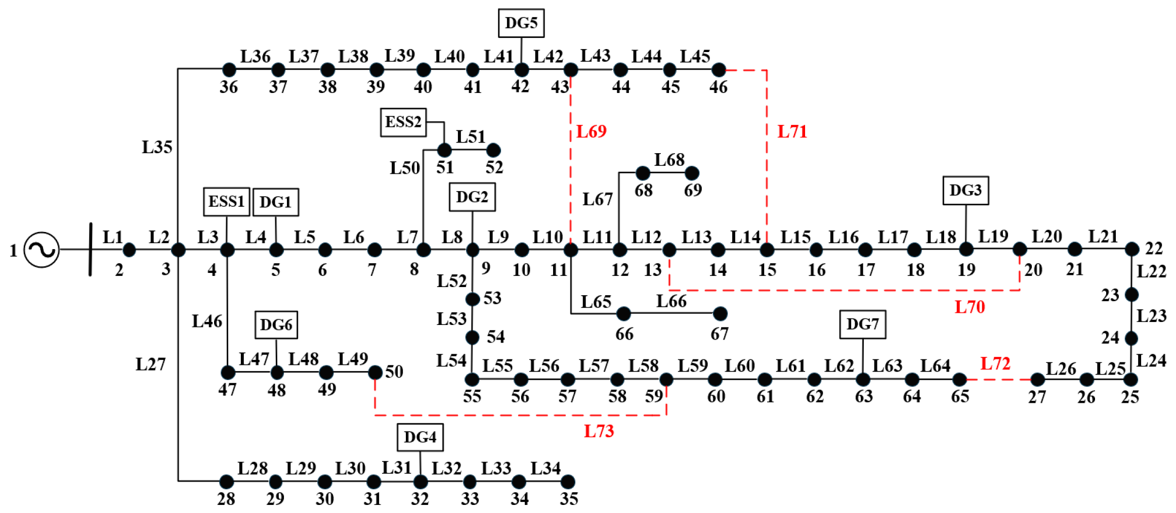
Appendix B.1. IEEE 69-Bus Distribution Network System with DGs

Table A1 lists the access nodes and parameters of the distributed power sources. In addition, the maximum allowable short-circuit current Imax of DGs is 1.2 times the rated current.
Table A1. Parameters of DGs in the IEEE 69-bus system.
EquipmentConnected NodeRated Active Power (kW)EquipmentConnected NodeRated Active Power (kW)
DG15800DG542200
DG29400DG648100
DG319250DG763800
DG432250
Table A2 lists the energy storage access nodes and parameters.
Table A2. Parameters of energy storage devices in the IEEE 69-bus system.
EquipmentConnected NodeCapacity (MWh)Upper Limit of Charging and Discharging Power (MW)Charging and Discharging Efficiency
Energy storage 141.20.45/0.4590%/90%
Energy storage 25110.3/0.390%/90%
The total load of the system is 3 802 kW + j2 695 kVar, and the load weights of each node are shown in Table A3.
Table A3. Parameters of loads in the IEEE 69-bus system.
Type of LoadConnected NodesWeight Factor
Primary load6, 8, 21, 51100
Secondary load12, 17, 33, 42, 49, 6410
Tertiary loadThe rest of the nodes1
Figure A1 shows the power prediction curves of DGs and loads in one day, where the ordinate refers to the DG output power as a percentage of the rated power, and the load demand power as a percentage of the maximum demand. The fuzzy triangle membership parameters of DGs, k i , 1 t are k i , 2 t , 0.92 and 1.08, respectively, and the fuzzy triangle membership parameters of loads, k i , 1 t   k i , 2 t , are 0.95 and 1.05, respectively.
Figure A1. DG and load power forecasting curves.
Electronics 14 01872 g0a1

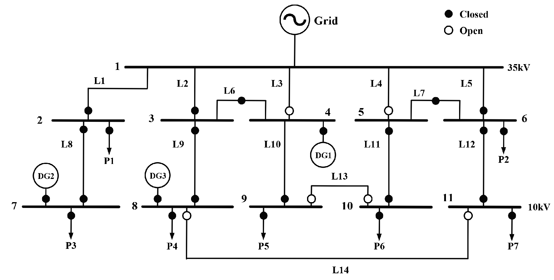
Appendix B.2. 11-Bus Distribution Network System with DGs

The system voltage level is 10 kV, and the power forecast of DGs and loads in one day is the same as that of system 1.
Table A4 lists the access nodes and parameters of the distributed power sources. In addition, the maximum allowable short-circuit current Imax of DGs is 1.2 times the rated current.
Table A4. Parameters of DGs in the 11-bus system.
EquipmentConnected NodeRated Active Power (MW)
DG144
DG2710.6
DG385
Table A5 lists the load weights of each node.
Table A5. Parameters of loads in the 11-bus system.
EquipmentConnected NodePower (MW)Weight Factor
P122.14 MW + j0.35 MVar100
P261.89 MW + j0.96 MVar100
P374.29 MW + j1.34 MVar100
P485.93 MW + j4.27 MVar10
P596.34 MW + j4.71 MVar1
P6104.16 MW + j1.35 MVar1
P7117.85 MW + j2.23 MVar1

References

  1. Morales-Munoz, A.; Freijedo, F.D.; Pugliese, S.; Liserre, M. Selective Virtual Impedance for Overcurrent Limitation in Grid-Forming Inverters Under Asymmetrical Faults. In Proceedings of the 2024 IEEE 15th International Symposium on Power Electronics for Distributed Generation Systems (PEDG), Luxembourg, 23–26 June 2024; pp. 1–5. [Google Scholar] [CrossRef]
  2. Liyanage, C.; Nutkani, I.; Meegahapola, L. A Comparative Analysis of Prominent Virtual Synchronous Generator Strategies Under Different Network Conditions. IEEE Open Access J. Power Energy 2024, 11, 178–195. [Google Scholar] [CrossRef]
  3. Shobug, M.A.; Chowdhury, N.A.; Hossain, M.A.; Sanjari, M.J.; Lu, J.; Yang, F. Virtual Inertia Control for Power Electronics-Integrated Power Systems: Challenges and Prospects. Energies 2024, 17, 2737. [Google Scholar] [CrossRef]
  4. Li, J.; Mo, H.; Sun, Q.; Wei, W.; Yin, K. Distributed Optimal Scheduling for Virtual Power Plant with High Penetration of Renewable Energy. Int. J. Electr. Power Energy Syst. 2024, 160, 110103. [Google Scholar] [CrossRef]
  5. Taheri, S.I.; Salles, M.B.C.; Costa, E.C.M. Optimal Cost Management of Distributed Generation Units and Microgrids for Virtual Power Plant Scheduling. IEEE Access 2020, 8, 208449–208461. [Google Scholar] [CrossRef]
  6. ALAhmad, A.K.; Verayiah, R.; Shareef, H. Long-Term Optimal Planning for Renewable Based Distributed Generators and Battery Energy Storage Systems toward Enhancement of Green Energy Penetration. J. Energy Storage 2024, 90, 111868. [Google Scholar] [CrossRef]
  7. Nsaif, Y.M.; Lipu, M.S.H.; Ayob, A.; Yusof, Y.; Hussain, A. Fault Detection and Protection Schemes for Distributed Generation Integrated to Distribution Network: Challenges and Suggestions. IEEE Access 2021, 9, 142693–142717. [Google Scholar] [CrossRef]
  8. Karimi, A.; Nayeripour, M.; Abbasi, A.R. Coordination in Islanded Microgrids: Integration of Distributed Generation, Energy Storage System, and Load Shedding Using a New Decentralized Control Architecture. J. Energy Storage 2024, 98, 113199. [Google Scholar] [CrossRef]
  9. Behbahani, M.R.; Jalilian, A.; Bahmanyar, A.; Ernst, D. Comprehensive Review on Static and Dynamic Distribution Network Reconfiguration Methodologies. IEEE Access 2024, 12, 9510–9525. [Google Scholar] [CrossRef]
  10. Zidan, A.; Khairalla, M.; Abdrabou, A.M.; Khalifa, T.; Shaban, K.; Abdrabou, A.; El Shatshat, R.; Gaouda, A.M. Fault Detection, Isolation, and Service Restoration in Distribution Systems: State-of-the-Art and Future Trends. IEEE Trans. Smart Grid 2017, 8, 2170–2185. [Google Scholar] [CrossRef]
  11. Shen, F.; Wu, Q.; Xue, Y. Review of Service Restoration for Distribution Networks. J. Mod. Power Syst. Clean Energy 2020, 8, 1–14. [Google Scholar] [CrossRef]
  12. Zarei, S.F.; Parniani, M. A Comprehensive Digital Protection Scheme for Low-Voltage Microgrids with Inverter-Based and Conventional Distributed Generations. IEEE Trans. Power Deliv. 2017, 32, 441–452. [Google Scholar] [CrossRef]
  13. Musarrat, M.N.; Fekih, A.; Islam, M.R. An Improved Fault Ride Through Scheme and Control Strategy for DFIG-Based Wind Energy Systems. IEEE Trans. Appl. Supercond. 2021, 31, 1–6. [Google Scholar] [CrossRef]
  14. Bagherzadeh, L.; Shayeghi, H.; Pirouzi, S.; Shafie-khah, M.; Catalão, J.P.S. Coordinated Flexible Energy and Self-Healing Management According to the Multi-Agent System-Based Restoration Scheme in Active Distribution Network. IET Renew. Power Gener. 2021, 15, 1765–1777. [Google Scholar] [CrossRef]
  15. Ye, Z.; Chen, C.; Chen, B.; Wu, K. Resilient Service Restoration for Unbalanced Distribution Systems With Distributed Energy Resources by Leveraging Mobile Generators. IEEE Trans. Ind. Inform. 2021, 17, 1386–1396. [Google Scholar] [CrossRef]
  16. Shi, X.; Zhang, H.; Wei, C.; Li, Z.; Chen, S. Fault Modeling of IIDG Considering Inverter’s Detailed Characteristics. IEEE Access 2020, 8, 183401–183410. [Google Scholar] [CrossRef]
  17. Cao, Y.; Liu, W.; Zhang, Y.; Zhang, H. An Improved Fault Recovery Strategy for Active Distribution Network Considering LVRT Capability of DG. In Proceedings of the 8th Renewable Power Generation Conference (RPG 2019), Shanghai, China, 24–25 October 2019; pp. 1–7. [Google Scholar]
  18. Li, C.; Xi, Y.; Lu, Y.; Liu, N.; Chen, L.; Ju, L.; Tao, Y. Resilient Outage Recovery of a Distribution System: Co-Optimizing Mobile Power Sources with Network Structure. Prot. Control Mod. Power Syst. 2022, 7, 32. [Google Scholar] [CrossRef]
  19. Lin, C.; Chen, C.; Bie, Z.; Li, G. Post-disaster Load Restoration Method for Urban Distribution Network with Dynamic Uncertainty and Frequency-Voltage Control. Autom. Electr. Power Syst. 2022, 46, 56–64. [Google Scholar]
  20. Shi, X.; Ke, Q.; Lei, J.; Yuan, Z. Fault Reconfiguration of Distribution Networks with Soft Open Points Considering Uncertainties of Photovoltaic Outputs and Loads. J. Phys. Conf. Ser. 2020, 1578, 012205. [Google Scholar] [CrossRef]
  21. Shen, Y.; Wang, G.; Zhu, J. Resilience Improvement Model of Distribution Network Based on Two-Stage Robust Optimization. Electr. Power Syst. Res. 2023, 223, 109559. [Google Scholar] [CrossRef]
  22. Kanojia, S.S.; Suthar, B.N. Voltage Stability Index: A Review Based on Analytical Method, Formulation and Comparison in Renewable Dominated Power System. IJAPE 2024, 13, 508. [Google Scholar] [CrossRef]
  23. Moradi, M.H.; Abedini, M. A Combination of Genetic Algorithm and Particle Swarm Optimization for Optimal Distributed Generation Location and Sizing in Distribution Systems with Fuzzy Optimal Theory. Int. J. Green Energy 2012, 9, 641–660. [Google Scholar] [CrossRef]
  24. Bi, C.Q.; Chen, J.J.; Wang, Y.X.; Feng, L. Fuzzy Credibility Chance-Constrained Multi-Objective Optimization for Multiple Transactions of Electricity–Gas–Carbon under Uncertainty. Electr. Power Syst. Res. 2025, 238, 111089. [Google Scholar] [CrossRef]
  25. Xiao, G.; Liu, H.; Nabatalizadeh, J. Optimal Scheduling and Energy Management of a Multi-Energy Microgrid with Electric Vehicles Incorporating Decision Making Approach and Demand Response. Sci. Rep. 2025, 15, 5075. [Google Scholar] [CrossRef] [PubMed]
  26. Fan, G.; Peng, C.; Wang, X.; Wu, P.; Yang, Y.; Sun, H. Optimal Scheduling of Integrated Energy System Considering Renewable Energy Uncertainties Based on Distributionally Robust Adaptive MPC. Renew. Energy 2024, 226, 120457. [Google Scholar] [CrossRef]
  27. Arjomandi-Nezhad, A.; Fotuhi-Firuzabad, M.; Moeini-Aghtaie, M.; Safdarian, A.; Dehghanian, P.; Wang, F. Modeling and Optimizing Recovery Strategies for Power Distribution System Resilience. IEEE Syst. J. 2021, 15, 4725–4734. [Google Scholar] [CrossRef]
  28. Kong, F.; Guo, T.; Zhang, X. Design of Active Fault Diagnosis and Repair System for Active Distribution Networks Based on Decision Tree Algorithm. In Proceedings of the 6th International Conference on Information Technologies and Electrical Engineering, Hunan, China, 3–5 November 2023; Association for Computing Machinery: New York, NY, USA, 2024; pp. 759–764. [Google Scholar]
  29. Wang, Q.; Meng, L. Distribution Network Fault Reconfiguration with Distributed Generation Based on Ant Colony Algorithm. Adv. Mater. Res. 2013, 732–733, 1328–1333. [Google Scholar] [CrossRef]
  30. Rebollal, D.; Carpintero-Rentería, M.; Santos-Martín, D.; Chinchilla, M. Microgrid and Distributed Energy Resources Standards and Guidelines Review: Grid Connection and Operation Technical Requirements. Energies 2021, 14, 523. [Google Scholar] [CrossRef]
  31. IEEE Std 1547-2018 (Revision of IEEE Std 1547-2003); IEEE Standard for Interconnection and Interoperability of Distributed Energy Resources with Associated Electric Power Systems Interfaces. IEEE: New York, NY, USA, 2018; pp. 1–138. [CrossRef]
  32. Li, H.; Deng, C.; Zhang, Z.; Liang, Y.; Wang, G. An Adaptive Fault-Component-Based Current Differential Protection Scheme for Distribution Networks with Inverter-Based Distributed Generators. Int. J. Electr. Power Energy Syst. 2021, 128, 106719. [Google Scholar] [CrossRef]
  33. Xu, C.; Dong, S.; Zhu, J. Description Method of Radial Constraints for Distribution Network Based on Disconnection Condition of Power Supply Loop. Autom. Electr. Power Syst. 2019, 43, 82–94. [Google Scholar]
  34. Ding, W.; Chen, Q.; Dong, Y.; Shao, N. Fault Diagnosis Method of Intelligent Substation Protection System Based on Gradient Boosting Decision Tree. Appl. Sci. 2022, 12, 8989. [Google Scholar] [CrossRef]
  35. Shan, W.; Li, D.; Liu, S.; Song, M.; Xiao, S.; Zhang, H. A Random Feature Mapping Method Based on the AdaBoost Algorithm and Results Fusion for Enhancing Classification Performance. Expert Syst. Appl. 2024, 256, 124902. [Google Scholar] [CrossRef]
  36. Han, Y.; Xu, K.; Qin, J. Based on the CART Decision Tree Model of Prediction and Classification of Ancient Glass-Related Properties. Highlights Sci. Eng. Technol. 2023, 42, 18–27. [Google Scholar] [CrossRef]
  37. Hu, H.; Siala, M.; Hebrard, E.; Huguet, M.-J. Learning Optimal Decision Trees with MaxSAT and Its Integration in AdaBoost. In Proceedings of the Twenty-Ninth International Joint Conference on Artificial Intelligence, International Joint Conferences on Artificial Intelligence Organization, Yokohama, Japan, 11–17 July 2020; pp. 1170–1176. [Google Scholar]
  38. Chen, S.; Shen, B.; Wang, X.; Yoo, S.-J. A Strong Machine Learning Classifier and Decision Stumps Based Hybrid AdaBoost Classification Algorithm for Cognitive Radios. Sensors 2019, 19, 5077. [Google Scholar] [CrossRef] [PubMed]
  39. Aboshady, F.M.; Pisica, I.; Zobaa, A.F.; Taylor, G.A.; Ceylan, O.; Ozdemir, A. Reactive Power Control of PV Inverters in Active Distribution Grids With High PV Penetration. IEEE Access 2023, 11, 81477–81496. [Google Scholar] [CrossRef]
  40. Bhutta, M.S.; Sarfraz, M.; Ivascu, L.; Li, H.; Rasool, G.; ul Abidin Jaffri, Z.; Farooq, U.; Ali Shaikh, J.; Nazir, M.S. Voltage Stability Index Using New Single-Port Equivalent Based on Component Peculiarity and Sensitivity Persistence. Processes 2021, 9, 1849. [Google Scholar] [CrossRef]
Figure 1. Standard requirements for LVRT capability of DG.
Electronics 14 01872 g001
Figure 2. Two-stage fault reconfiguration strategy for distribution network with DGs.
Electronics 14 01872 g002
Figure 3. Flow chart of fast solution algorithm for power restoration strategy based on decision trees.
Electronics 14 01872 g003
Figure 4. An IEEE 69-bus distribution network with DGs.
Electronics 14 01872 g004
Figure 5. A real-world 11-bus distribution network.
Electronics 14 01872 g005
Figure 6. L ˜ i j change diagram of reconstructed system under L3 line fault.
Electronics 14 01872 g006
Figure 7. Comparison of load recovery results with/without considering FRT.
Electronics 14 01872 g007
Table 1. The fault cases of the 69-bus system.
Case NumberFaulty Line
1L3
2L10
3L5 and L18
4L38 and L64
5L48; DG6 fault ride-through operation
6L62; DG7 fault ride-through operation
Table 2. The fault cases of the 11-bus system.
Case NumberFaulty Line
1L2
2L9
3L3 and L10
4L4; DG1 fault ride-through operation
Table 3. Load recovery results of 69-bus system.
Case
Number
Reconfiguration
Operation
Load Recovery Percentage
Primary LoadSecondary LoadTertiary Load
1L69 is closed100%100%90.57%
2L71 is closed100%100%100%
3L69 and L72 are closed100%100%81.33%
4L69 and L72 are closed100%100%100%
5L73 is closed100%100%93.04%
6L72 is closed100%100%95.48%
Table 4. Load recovery results of 11-bus system.
Case
Number
Reconfiguration
Operation
Load Recovery Percentage
Primary LoadSecondary LoadTertiary Load
1L11 is closed100%100%100%
2L14 is closed100%100%100%
3L12 and L13 are closed100%100%100%
4L11 is closed100%100%100%
Table 5. The results of the 69-bus system reconfiguration.
Case
Number
Reconfiguration
Operation
The   Worst   L ˜ i j Loss of Load (MWh)
1L69 is closed−0.88981.4664
2L69 is closed−0.92640.4602
3L72 and L73 are closed−0.94791.2070
4L69 and L72 are closed−0.92510.6349
Table 6. The results of the 11-bus system reconfiguration.
Case
Number
Reconfiguration
Operation
The   Worst   L ˜ i j Loss of Load (MWh)
1L11 is closed−0.99840
2L14 is closed−0.99190
3L12 and L13 are closed−0.99190
Table 7. The results with different weight settings of voltage stability and load shedding.
ω1/ω2Reconfiguration
Operation
Worst   L ˜ i j Loss of Load (MWh)
0.1/0.9L72 and L73 are closed−0.94791.2070
0.4/0.6L72 and L73 are closed−0.94791.2070
0.9/0.1L72 and L73 are closed−0.94791.2070
Table 8. Comparison of the reconfiguration results of the different algorithms.
Case NumberReconfiguration Results of Conventional Mathematical OptimizationReconfiguration Results of Ordinary Decision TreesReconfiguration Results of AdaBoost-Enhanced Decision Trees
1L69 is closedL69 is closedL69 is closed
2L71 is closedL71 is closedL71 is closed
3L69 and L72 are closedL70 and L73 are closedL69 and L72 are closed
4L69 and L72 are closedL71 and L72 are closedL69 and L72 are closed
5L73 is closedL73 is closedL73 is closed
6L72 is closedL72 is closedL72 is closed
Table 9. Comparison of the solving time of the different algorithms.
Case NumberSolving Time of Conventional Mathematical Optimization (s)Solving Time of AdaBoost-Enhanced Decision Trees (s)
125.68610.2426
223.57070.2815
327.76530.2328
424.33910.3042
522.91840.2436
625.51020.2761
7Non-convergence0.2591
Table 10. Comparison of optimal reconfiguration results with and without considering uncertainty.
Case
Number
Considering UncertaintyWithout Considering Uncertainty
Worst   L ˜ i j Loss of Load (MWh) Worst   L ˜ i j Loss of Load (MWh)
1−0.88981.4664−0.88981.4664
2−0.92640.4602−0.92640.4712
3−0.94791.2070−0.84251.5457
4−0.92510.6349−0.92510.7266
Disclaimer/Publisher’s Note: The statements, opinions and data contained in all publications are solely those of the individual author(s) and contributor(s) and not of MDPI and/or the editor(s). MDPI and/or the editor(s) disclaim responsibility for any injury to people or property resulting from any ideas, methods, instructions or products referred to in the content.

