Interaction Scenarios Considering Source–Grid–Load–Storage for Distribution Network with Multiple Subjects and Intelligent Transportation Systems

Abstract

With the spread of electric vehicles (EVs), the EV load will have a significant impact on the planning and operation of the grid and the operation of the electricity market. Due to the charging and discharging characteristics of EVs, as well as their randomness and dispersion, it is feasible and challenging to introduce EV loads into the grid as a means of frequency regulation and peak shaving of the power system. In this paper, considering multi-subject distribution networks and the interaction of source–grid–load–storage with Intelligent Transportation Systems (ITS), a density peak clustering (DPC) algorithm based on principal component analysis is employed to analyze the spatial and temporal characteristics of EV loads and identify the access status of EV charging stations and EV load status in each region in real time, as well as analyze the adjustable capacity and adjustable range of EV loads. Based on the adjustable capacity of the EV load, the optimization objectives include the maximum regulation of the EV load and the most economical operation cost. An accurate load regulation strategy based on automatic active control (APC) is proposed to reduce the maximum frequency deviation by 25% by integrating the load regulation of electric vehicles into the original AGC frequency regulation. At the same time, the feasibility of electric vehicles in peaking and standby scenarios is studied and verified through simulation cases, which can reduce the peak value of thermal power generation by 15% and 10% in the morning and evening.

1. Introduction

To align with the national “double carbon” goal and support the development of clean energy, a new paradigm for power systems, centered on renewable energy sources, is being constructed. This initiative corresponds to the National Grid’s “Carbon Peak, Carbon Neutral” action program, aiming to accelerate the transformation of energy production and consumption. Within the realm of electrical engineering, the synergy and interaction among sources, grid infrastructure, loads, and storage have emerged as prominent research directions. This interaction serves as a critical component in realizing the energy Internet. In Ref. [1], investigating adjustable load resources represents an effective strategy to enhance power system stability, mitigate carbon emissions, and achieve the objectives of the “double carbon” initiative. Amidst a suite of supportive policies championed by the Chinese government to foster cleaner transportation, the industrial technology and business models of EVs are experiencing robust and well-regulated growth [2].

With the widespread adoption of EVs, their integration into the electrical grid as loads will exert a significant impact on grid planning, operation, and the electricity market [3,4]. Large-scale EV deployment signifies a significant accumulation of stored-load resources. The energy storage capacity inherent in EV batteries provides users with flexibility in choosing charging times, thereby rendering the charging load somewhat manageable. Effective charging control serves not only to mitigate and eliminate adverse effects of EVs on the power grid but also bolsters grid operations, enhancing efficiency, safety, economic viability, and operational flexibility.

Currently, research efforts are underway regarding the involvement of EV loads in auxiliary services such as frequency regulation, peak shifting, and standby operations. In the literature, Ref. [5] designed a hybrid deep charge–fusion model, integrating spatial, temporal, and demographic factors to predict charging behavior, which can effectively support further energy control. Ref. [6] employed a continuous-time model (CTM) to facilitate the participation of EV loads in power system scheduling services. However, this study lacks an analysis of the spatiotemporal coupling of EV loads. Ref. [7] proposed a charge and discharge incentive mechanism for EV clusters and established a multi-variety market operating income optimization model considering multi-stage time series interaction but lacked the effect of the peak–valley difference of electricity price on the incentive effect and the geospatial analysis. Ref. [8] proposed a novel data-driven and machine learning-based two-layer aggregation dispatchable capacity modeling method, considering various levels and scenarios of power system regulation and control, but the economic consideration of electric vehicles participating in auxiliary services is very rough, and the cost–benefit analysis is not carried out. Ref. [9] suggested a control framework for clustered EVs to engage in system frequency modulation (FM) utilizing Butterworth decomposers. However, the article’s economy, spatial and temporal distribution, and actual data verification are completely missing, and the applicability and multi-scenario coverage are insufficient. Ref. [10] innovatively applied VSM technology to the charge and discharge control of electric vehicles and designed the control architecture of the two-stage bidirectional charge and discharge machine, but the spatial characteristics are not considered, and the time characteristics are roughly described. The conclusion is that this strategy can reduce the frequency modulation resource demand of the microgrid and reduce the investment cost but it is not quantified. Ref. [11] proposed a charging regulation strategy in which electric vehicle clusters participate in the FM auxiliary service market. Combined with the PJM market mechanism, the economic and FM effects are verified. However, the scenario coverage is limited, and the spatiotemporal characteristics analysis of electric vehicles is not involved. Ref. [12] innovatively combined VSM technology with fuzzy control to achieve intelligent regulation and control of EV charging and discharging, effectively balancing the frequency modulation needs of the power grid and the charging needs of users. However, the economy and temporal and spatial distribution characteristics are not discussed, and the charging behavior is simulated through truncated normal distribution, lacking calibration with actual user behavior. A detailed dimension comparison of the above methods is shown in

Table 1. Comparison of electric vehicles participating in power grid regulation.

Literature	Strategy Dynamics	Economic	Spatiotemporal Distribution	Applicability	Actual Data Verification	Multi-Scenario
This paper	√	√	√	√	√	√
[6]	√	√
[7]		√	√	√		√
[8]	√		√	√	√	√
[9]	√					√
[10]	√			√		√
[11]	√	√		√	√
[12]	√			√		√

.

Traditional methods usually assume that the load is static and do not take into account the real-time changes in the charging state of EVs, which makes it difficult to apply in the actual regulation of power grids. In addition, most of the scheduling decision optimization methods stay at the theoretical level, not combined with the actual operation of the power system, and lack applicability.

In this paper, a DPC algorithm based on principal component analysis is proposed to analyze the spatiotemporal distribution characteristics of electric vehicle load in different types and different locations so as to identify the access status of electric vehicle charging stations and the charging status of electric vehicles in each region in real time. In addition, this study integrates the adjustable capacity of electric vehicle load with the dynamic zoning of a power system to reduce the voltage fluctuation of the power grid, introduces the frequency modulation of electric vehicle load into the existing AGC frequency modulation framework, and, finally, proposes a two-stage optimal accurate load regulation strategy based on APC to optimize the maximum load regulation and cost efficiency. Compared with the traditional AGC method, the maximum frequency deviation can be reduced by 25%. In addition, the feasibility of electric vehicles in peak load and standby scenarios is also discussed, which can significantly reduce the peak value of thermal power generation in the morning and evening, reaching 15% and 10%, respectively.

2. Analysis of Electric Vehicle Load Adjustable Capacity

In this article, the model construction of electric vehicles and batteries is based on the following assumptions:

(1)

It is assumed that users’ willingness to participate in grid auxiliary services (such as frequency modulation and peak clipping) remains unchanged during the dispatching cycle. That is, the user will not quit or change the participation status during the charging process.

(2)

The SOC limit and the ramp rate of charge and discharge power of the battery in the model are fixed values. Considering the battery life, the SOC limit value is determined with reference to other studies.

(3)

In the APC framework, it is assumed that the communication link between the charging pile, the vehicle networking platform, and the dispatching center has no delay and no packet loss, and the data collection is completely synchronized.

2.1. Single Load Model of EV

The state of charge (SOC) of EV refers to the ratio of the remaining battery capacity E to its rated capacity Emax.

Unidirectional charging with adjustable power ΔP is obtained as follows:

$$\Delta P=X*\min \{P_{bi},P_{\max i}-P_{bi}\}$$

(1)

In Equation (1), $P_{\max i}$ sets the power limit for charging pile discharges, $P_{bi}$ sets the base power for charging the first vehicle, and X means the willingness of users to participate in FM services or not.

The power of the EV during charging can be adjusted in the [P_bi − ΔP, P_bi + ΔP] interval to ensure that the charging power is continuously positive and provide equal-sized upward and downward regulation of the standby, that the SOC is monotonically increasing, and that participation in the FM does not affect its normal charging.

The adjustable power for two-way charging is obtained as follows:

$$DP=X*P_{maxi}$$

(2)

2.2. Adjustable Capacity Evaluation Method for EVs

Whether or not there is room for upward adjustment of the charging and discharging power of EVs is mainly limited by the travel power demand of EV users and battery life. The charging power can be further reduced or more power can be released only when the user’s demand is satisfied, the depth of discharge is within the permissible range, and the current power is less than the maximum discharge power.

In order to ensure that the EV leaves with the power SOCi need desired by the user, after the scheduling of Δt, the EV’s power at the moment t + Δt has to be greater than the minimum power SOCi min; the allowed t + Δt is calculated by Equation (3) [13].

$$\begin{array}{l}SO{C}_{\min ,t+\Delta t}^i=SO{C}_{need}^i-\\ {\displaystyle \frac{(-P_{\max i})\times {\eta }_{char}\times (T_{dep,i}-(t+\Delta t))}{C_i}}\times 100\%\end{array}$$

(3)

where C_i is the battery capacity, η_char is the EV charging efficiency, and T_dep,i is the moment of departure of the first EV.

When the battery level is greater than $SO{C}_{\min ,t+\Delta t}^i$, and thereafter, if the EV is continuously charged at maximum power, it is able to reach the user’s desired level of charge when it is scheduled to leave. Otherwise, the user demand cannot be reached.

Battery life can be expressed by the number of cycles of charging and discharging under certain working conditions; the depth of discharge is inversely proportional to the cycle life, and the greater the depth of discharge, the shorter the cycle life will be. Therefore, in order to protect the battery life, it is necessary to come in to avoid frequent deep charging and discharging and at the same time to provide more dispatchable capacity. According to Ref. [9], set the depth of discharge for the primary FM to 50% and the depth of discharge for the secondary FM to 60%. At moment $t+\Delta t$, the EV charge must not fall below 100%-$D_{\max }$, where $D_{\max }$ denotes the depth of discharge.

$$SO{C}_{\min ,t+\Delta t}^i\ge 100\%-D_{\max }$$

(4)

As can be seen from Figure 1, when $P_{\max i}>P_{bi}$, it indicates that at this time the EV charging and discharging power has upward space, i.e., the actual upward capacity of EVs can be adjusted as follows:

$$\Delta P_{up}^i=P_{\max i}-P_{bi}$$

(5)

Scalable EVs have an upwardly adjustable capacity $P_{total,up}$ of:

$$P_{total,up}={\displaystyle \sum _{i=1}^N\Delta P_{up}^i}$$

(6)

The potential for downward adjustment in EV (EV) charging and discharging power is primarily constrained by both the maximum charging capacity of the charging infrastructure and the limitations imposed by the battery’s power capacity. It is only feasible to increase the charging power further if it remains below the maximum charging capacity and if the battery is not yet fully charged. This capability provides a reserve capacity that can be adjusted downward, offering flexibility to the grid. Battery power constraints are shown as follows:

$$SO{C}_{t+\Delta t}^i\le 100\%$$

(7)

The maximum value of power that can be added to an EV is obtained as follows:

$$\Delta SO{C}_t^i=100\%-SO{C}_t^i$$

(8)

Therefore, the maximum charging power allowed for an EV is obtained as follows:

$$P_{\Delta t}^i=\max (P_{\max i},-{\displaystyle \frac{\Delta SO{C}_t^i\times C_i}{{\eta }_{char}\times \Delta t}})$$

(9)

As depicted in Figure 1, the graph illustrates that the EV charging and discharging power at this juncture can be further optimized, implying that the real-time adjustable downward capacity of the EV can be determined as follows:

$$\Delta P_{down}^i=P_{\max i}+P_{bi}$$

(10)

The downsizable capacity of a scaled EV can be expressed as follows:

$$P_{total,down}={\displaystyle \sum _{i=1}^N\Delta P_{down}^i}$$

(11)

2.3. DPC Method

The DPC algorithm incorporates two pivotal concepts: local density and relative distance [12,14]. Local density is computed based on a provided dataset, where N represents the number of samples and M denotes the number of dimensions in the sample space [15,16,17,18]. The local density of a sample point i can be determined through two methods: utilizing a truncated kernel for discrete values or employing a Gaussian kernel for continuous values [10]. The Gaussian kernel is expressed as shown in Equation (12):

$${\rho }_i={\displaystyle \sum _{i\ne j}\exp \left[-{\left(\frac{d_{ij}}{d_c}\right)}^2\right]}$$

(12)

The variable d_ij represents the Euclidean distance between data point i and data point j, while d_c denotes the truncation distance. Regarding relative distance, for the densest sample, the relative distance is defined as shown in Equation (13):

$${\delta }_i=\underset{i\ne j}{\min }(d_{ij})$$

(13)

The relative distance $\delta i$ refers to the minimum distance between sample point i and other points possessing higher density. Prior to computing the sample point i, it is necessary to rank the local density of each data point.

The steps of the DPC algorithm involve constructing the distance matrix, determining the value of $d_c$, calculating local density and relative distances, and iterating or terminating the loop based on testing criteria. The schematic diagram illustrating the program for evaluating the adjustable load capacity of EVs is presented in Figure 2.

3. Dynamic Zoning Method of Power Grid

When scaling up EV loads, it is imperative to comprehensively consider the spatially uneven distribution of the adjustable load capacities of EVs. This necessitates a real-time analysis of grid current distribution and the geographical dispersion of dispatchable EV load resources in conjunction with grid operational conditions and scheduling capacity demands. To address this, a temporal and spatial decoupling of the power grid is required, entailing research into dynamic grid partitioning through continuous rolling control. This involves considering reactive/active balance indices and coupling indices of nodes within the area, followed by ongoing optimization at hourly intervals to effect dynamic grid partitioning. Post-partitioning, grid trend calculations are conducted to assess the impact of dynamic partitioning measures on stability indices such as line load ratios and regional reserve capacities. This rigorous analysis enables the effective evaluation of the rationality of grid regulation and control under dynamic partitioning conditions [19,20,21].

3.1. Power System Zoning Principles

The power system zoning must adhere to the following principles:

(1)

Ensure strong electrical coupling among nodes within each sub-area and weak coupling between sub-areas to minimize the mutual influence of reactive voltage control across sub-areas.

(2)

Maintain power balance and reserve a certain amount of regulation power within each sub-area while allocating dynamic scheduling resources reasonably.

(3)

Maintain connectivity among nodes within the same partition, ensuring direct or indirect connections between them rather than through nodes outside the partition.

(4)

Avoid isolated nodes by including at least two nodes in each partition and ensuring no duplicate nodes within each partition.

3.2. Extended Voltage Sensitivity Matrix

As documented in the literature [22], an enhanced sensitivity matrix has been employed for partitioning, capable of encompassing the coupling relationships among all nodes while simultaneously reflecting the influence of active power on power system voltage.

For PQ nodes, specified by active power $P_{ic}$ and reactive power $Q_{ic}$, the power equations in polar coordinates are as follows:

$$\Delta P_i=P_{ic}-U_i{\displaystyle \sum _{j=1}^n{U}_j(G_{ij}\cos {\delta }_{ij}+B_{ij}\sin {\delta }_{ij})}$$

(14)

$$\Delta Q_i=Q_{ic}-U_i{\displaystyle \sum _{j=1}^n{U}_j(G_{ij}\sin {\delta }_{ij}+B_{ij}\cos {\delta }_{ij})}$$

(15)

For the PV node, the known quantities are the active power $P_{ic}$ and voltage $U_{ic}$, while the reactive power $Q_{ic}$ remains unknown. Therefore, only the equations of $\Delta P_i$ are retained, as depicted in Equation (14).

Let the system comprise a total of n nodes, with m PQ nodes, n-m-1 PV nodes, and one balance node. Consequently, the power equation in polar coordinates comprises 2m PQ node equations and n-m-1 PV node equations, totaling n+m-1 equations. The number of unknowns equals the number of equations, enabling solvability by expanding and organizing the error equation based on the Taylor series.

The abbreviated block matrix form is given below:

$$[\begin{array}{c}\Delta P\\ \Delta Q\end{array}]=-[\begin{array}{cc}{H}_{(n-1)(n-1)}& N_{(n-1)m}\\ J_{m(n-1)}& L_{mm}\end{array}][\begin{array}{c}\Delta \delta \\ \Delta U/U\end{array}]$$

(16)

The N matrix and L matrix are capable of representing the coupling relationship between active and reactive power and the voltage magnitude of each node, respectively. The voltage sensitivity matrix encompassing all PQ load nodes is obtained by amalgamating the influences of active and reactive power on node voltages, as follows:

$$S_0=-{(L_{mm}+N_{mm})}^{-1}$$

(17)

As the N matrix is typically much smaller than the L matrix, reactive voltage control continues to play a dominant role in this sensitivity matrix. Moreover, it exclusively encompasses information from PQ load nodes, excluding details pertaining to PV power nodes and balancing nodes. Drawing upon relevant studies, each of the remaining nodes can be sequentially designated as PQ nodes, grouped together to yield n-m sensitivity matrices, as follows:

$$\begin{array}{l}{S}_x=-{(L_{(m+1){(m+1)}_x}+N_{(m+1){(m+1)}_x})}^{-1}\\ =[\begin{array}{cccc}{S}_{{11}_x}& \cdots & S_{1m_x}& S_{1{(m+1)}_x}\\ \cdots & \cdots & \cdots & \cdots \\ S_{m{1}_x}& \cdots & S_{m{m}_x}& S_{m{(m+1)}_x}\\ S_{(m+1)1_x}& \cdots & S_{(m+1)m_x}& S_{(m+1){(m+1)}_x}\end{array}]\end{array}$$

(18)

where x can take an integer between 1 and n-m.

The newly acquired n-m sensitivity matrices, alongside the initial PQ node sensitivity matrices, are amalgamated to form the final sensitivity matrix S. Firstly, the first mm elements of each sensitivity matrix are summed and averaged, resulting in an mm matrix representing individual trend states. Subsequently, the last row and column of each sensitivity matrix are successively appended to the bottom and right side of this matrix. Lastly, the bottom-right elements of each matrix are combined to form the bottom-right corner of the final sensitivity matrix, as follows:

$$S=[\begin{array}{cccccc}\overline{S_{11}}& \cdots & \overline{S_{1m}}& S_{1{(m+1)}_1}& \cdots & S_{1{(m+1)}_{n-m}}\\ \cdots & \cdots & \cdots & \cdots & \cdots & \cdots \\ \overline{S_{m1}}& \cdots & \overline{S_{mm}}& S_{m{(m+1)}_1}& \cdots & S_{m{(m+1)}_{n-m}}\\ S_{(m+1)1_1}& \cdots & S_{(m+1)m_1}& S_{(m+1){(m+1)}_1}& 0& 0\\ \cdots & \cdots & \cdots & 0& \cdots & 0\\ S_{(m+1)1_{n-m}}& \cdots & S_{(m+1)m_{n-m}}& 0& 0& S_{(m+1){(m+1)}_{n-m}}\end{array}]$$

(19)

3.3. Electrical Distance Matrix

The definition and calculation method of the electrical distance vary across different studies [23]. However, they all aim to quantify the strength of electrical coupling between nodes or regions. We refer to the relevant literature to define electrical distance as follows:

$$D_{ij}=\sqrt{{\displaystyle \sum _{k=1}^n{(\ln \frac{S_{ij}}{S_{i\max }}-\ln \frac{S_{ji}}{S_{j\max }})}^2}}$$

(20)

For the lower right region of the matrix, due to the presence of numerous zero elements, taking the logarithm may yield infinity, potentially overwhelming the data. Therefore, only the first m data points are utilized in its calculation, as follows:

$$D_{ij}=\sqrt{{\displaystyle \sum _{k=1}^m{(\ln \frac{S_{ij}}{S_{i\max }}-\ln \frac{S_{ji}}{S_{j\max }})}^2}}$$

(21)

So far, an n*n spatial electrical distance matrix D has been obtained, which encapsulates the coupling information of all nodes within the power system. In comparison to alternative methods of defining electrical distances, this calculation approach maps each node to a linear space. This not only reflects the electrical coupling relationship between any two nodes but also comprehensively considers the influence of other nodes on these two nodes.

3.4. Verification and Correction of Partitions

After obtaining the partitioning results, the first step should be to check whether there is an isolated node within it. If an isolated node is found, it should be merged into the partition with the smallest electrical distance. Subsequently, it is necessary to conduct power reserve calibration for each partition.

The active and reactive power reserves within each sub-area play a crucial role in ensuring the stability of the power system. The voltage at each node within the power system exhibits a strong coupling relationship with reactive power. An adequate dynamic reactive power reserve helps the grid manage voltage fluctuations resulting from various disturbances, thereby maintaining system voltage stability. Conversely, active power is closely tied to the frequency of the power system. The system requires a certain level of active reserve to manage load fluctuations and address various exceptional circumstances. Hence, the calibration of active and reactive power reserves within each area is imperative post-partitioning.

Following partitioning, the calibration of active and reactive power reserves in each region becomes necessary. Assuming the maximum total reactive power generation in region i is $Q_{Gi}$, the maximum total active power generation is $P_{Gi}$, the total reactive power demanded by the load in the region is $Q_{Li}$, and the total active power is $P_{Li}$, the reserve is calculated as follows:

Reactive power reserve:

$${\beta }_i=(1-{\displaystyle \frac{Q_{Li}}{Q_{Gi}}})\times 100\%$$

(22)

Active power reserve:

$${\alpha }_i=(1-{\displaystyle \frac{P_{Li}}{P_{Gi}}})\times 100\%$$

(23)

During actual system operation, each region should maintain a reactive power margin of at least 10~15% to prevent voltage collapse caused by insufficient reactive power [24]. Additionally, besides meeting anticipated load demands, active power reserves are required to ensure power quality and the safe, stable operation of the system in unforeseen circumstances. Typically, the reserve capacity in the system should be between 15% and 20% of the normal power supply capacity. This paper mandates that both reserves be above 20%. If the values fall below this threshold, corrective action is necessary.

After obtaining the partitioning results, the boundary nodes between two adjacent partitions are identified based on the topological structure of the power system. In cases where the power reserve in one partition is insufficient, it is possible to transfer the boundary load node between this partition and the neighboring partition with sufficient power reserve to the latter. This action serves to enhance the power reserve in the partition with insufficient reserves and promotes a more balanced distribution of power among the various partitions.

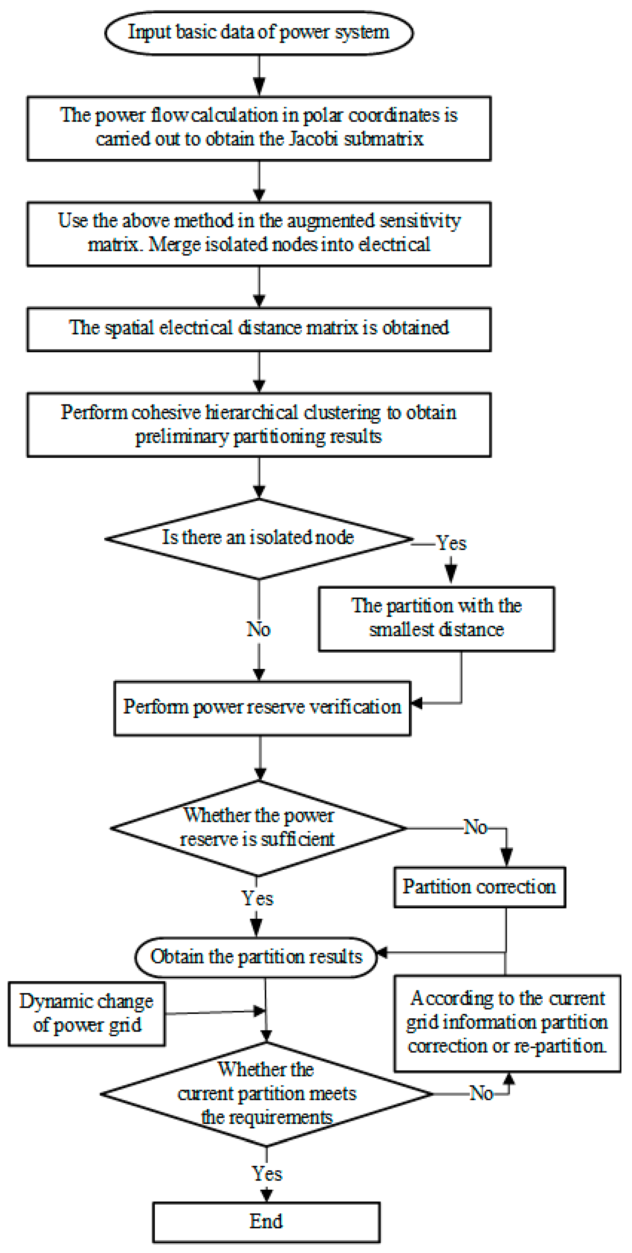
3.5. Dynamic Changes of Partitions

In the operation of a power system with a significant presence of EVs, power undergoes continuous real-time dynamic changes. Real-time dynamic rolling regulation can be carried out with a time granularity of five minutes. During each regulation cycle, the power reserve and node voltages in each partition of the system are calculated. If the power reserve is deemed sufficient and the node voltages remain stable, no adjustments are necessary, and the partition results from the previous time period are retained. However, if there is an insufficiency in power reserve or if the voltage exceeds specified limits, corrections are made using the method outlined in the preceding section. If this method proves ineffective, then re-partitioning is initiated from the beginning. The final dynamic partitioning process unfolds as follows in Figure 3:

4. EV Precision Regulation Framework

Different scenarios such as peak regulation, frequency regulation, standby, and others impose varying requirements on response speed, adjustable capacity, and other indicators of EV loads. To address these diverse demands while considering the current operating conditions of the power grid and the spatial and temporal distribution characteristics of EV load adjustable capacity, we extend AGC to APC. This extension aims to align grid dispatching demands with the response characteristics of EV loads, tracking their actual operating conditions. By matching grid scheduling demands with EV load response characteristics and monitoring their actual operations, the APC system calculates active system deviation in scenarios such as prediction errors or equipment failures. It then conducts rolling optimization of EV load regulation and control commands using APC algorithms, thereby achieving precise regulation and control of EV loads.

During normal operation of the APC system, data collection and transmission occur across multiple components. On the generation side, the Distributed Control System (DCS) gathers data, which are then relayed to the APC controller at the dispatch center via the Remote Terminal Unit (RTU). On the load side, the load aggregator’s Telematics platform collects information including charging station access data, adjustable capacity, upper and lower power limits, etc. These data are aggregated based on region and sent to the APC controller. Meanwhile, the grid operation data collection system gathers data such as grid frequency and power, transmitting them to the APC controller as well. Utilizing relevant algorithms, the APC controller processes the collected data to generate regulation and control commands for both generator groups and aggregated EV loads.

The control commands for the generator sets are dispatched to the DCS of the unit control system via RTUs, facilitating control over the generator sets. Conversely, the load control commands are transmitted to the vehicle networking platform of the load aggregator. The platform then disassembles the control commands and forwards them to the charging stations/piles, thereby enabling control over the EV loads. This iterative process is repeated to maintain the dynamic balance of grid power. The control logic block diagram of APC is depicted in Figure 4.

When the APC control strategy initiates execution, it initially retrieves monitoring data from the power generation, grid, and load sides of the system. These data enable a comprehensive description of the grid’s operational state, including the calculation of area power deviation based on the collected frequency deviation of the grid and integrating coefficients. To achieve optimal allocation of power regulation commands, the APC control strategy considers the system’s operating conditions and establishes a coordinated dispatch optimization model for generator sets and EV loads. Given the complexity of the model, it is simplified and solved using linear programming methods to efficiently address the model. Upon obtaining the optimal solution, the APC system dispatches control commands to the generator sets and the vehicle network platform accordingly. Subsequently, the APC control strategy cyclically reads grid operation data and repeats the aforementioned process to maintain a balance between generator output and load, ensuring the system’s safe and stable operation.

5. EV Load Participation System FM Model

To achieve optimal allocation of power regulation commands, the APC control strategy takes into account various factors, including the operating state of the generator set, the adjustable capacity of the aggregated EV load, the power grid’s operational conditions, and the economic cost of scheduling. Based on these considerations, it establishes a two-phase dispatch optimization model for the EV load. 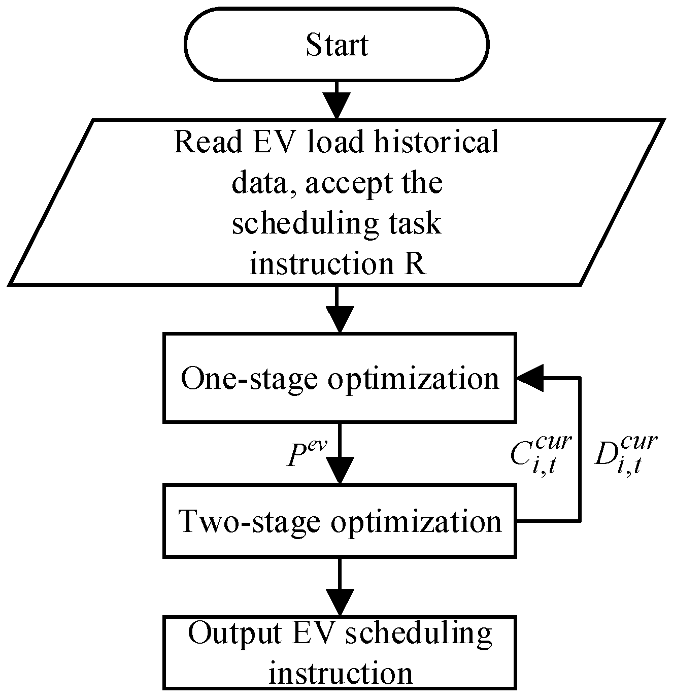Figure 5 depicts the program block diagram of APC, while Figure 6 illustrates the schematic diagram of the optimization model of the load frequency regulation module.

Table 2. Optimization variables.

Optimization Parameters	Definitions
$G_{i,t}^{veh}$	A binary variable (0–1) indicating whether the charging station participates in the load FM task at that time
$P_{i,t}^{veh}$	The charging power instruction value for charging station at time t
$C_{i,t}^{cur}$	The charging commands given to the charging station at time t
$D_{i,t}^{cur}$	The discharging commands given to the charging station at time t

and

Table 3. Constant variables.

Constant Variables	Definitions
$R(t)$	The FM task instruction issued by the dispatch center at the given time
$c_{i,t}^{veh}$	The operational cost coefficient for the charging station at time t
$C_{i,\max }^{\max }$	The rated charging power of the charging station
$D_{i,\max }^{\max }$	The maximum discharging power of the charging station
$P_{i,t,\max }^{veh}$	The maximum charging power for the charging station at time t
$P_{i,t,\min }^{veh}$	The minimum charging power for the charging station at time t
$E_{i,t,\max }^{veh}$	The lower limits of the battery power in the charging station
$E_{i,t,\min }^{veh}$	The lower limits of the battery power in the charging station
$P_L^t$	Load size except for electric vehicles
$E_{i,t-1}^{veh}$	The remaining power of the charging station at time t − 1

explain the meaning of each variable in the optimization algorithm [24].

5.1. Optimization Object

$$F=\min {\displaystyle \sum _i{\displaystyle \sum _t(R(t)-}}{G}_{i,t}^{veh}{P}_{i,t}^{veh})$$

(24)

The first-stage optimization objective F for load FM aims to maximize the participation of EV loads in FM.

$$f=\min {\displaystyle \sum _i{\displaystyle \sum _t{c}_{i,t}^{veh}(P_{i,t,\max }^{veh}-P_{i,t}^{veh})\Delta t}}$$

(25)

The second-stage optimization objective for EV FM aims to minimize the operational cost $f$ of load FM and enhance economic efficiency.

5.2. Constraint Condition

The constraints regarding the participation of EV loads in power system FM primarily encompass power balance and charging pile operation constraints.

(1)

System power load power balance.

The system’s power generation equals the real-time power demand. The main sources of power generation include thermal, gas, hydro, pumped storage, wind, and solar power. Additionally, there is power import/export from neighboring areas.

$${\displaystyle \sum _{\mathrm{i}\in B}{\displaystyle \sum _{j=1}^{N_i}{P}_{i,j}^t}}=P_L^t+{\displaystyle \sum _{i=1}^{N_{car}}{P}_{i,t}^{veh}}, \forall 1\le \mathrm{t}\le 24$$

(26)

B represents the type of generating units, where thermal power is denoted by subscript T, gas power by subscript G, hydro power by subscript H, pumped storage by subscript P, wind power by subscript W, solar power by subscript S, and external power import/export by subscript IN.

(2)

Charging pile operation constraints.

All charging piles need to meet the constraints of the upper and lower limits of the output of the charging pile itself.

$$C_{i,t}^{cur}\le C_{i,\max }^{\max }$$

(27)

$${\mathrm{D}}_{i,t}^{cur}\le D_{i,\max }^{\max }$$

(28)

$$P_{i,t}^{veh}=C_{i,t}^{cur}-D_{i,t}^{cur}$$

(29)

$$P_{i,t,\min }^{veh}\le P_{i,t}^{veh}\le P_{i,t,\max }^{veh}$$

(30)

$$E_{i,t,\min }^{veh}\le E_{i,t-1}^{veh}+P_{i,t-1}^{veh}\Delta t\le E_{i,t,\max }^{veh}$$

(31)

The upper and lower bounds of the charging station power are constrained as depicted in Equations (30)–(33).

(3)

Charging station operation constraints.

All charging stations must determine whether they are participating in FM at a given moment in time. To achieve this, a constraint involving binary (0–1) variables is introduced.

$$G_{i,t}^{veh}\in 0,1$$

(32)

6. System Peak Load Balancing and Standby Model

In the peak-shaving scenario, the primary objective is to conduct a daily operation simulation test to verify if existing units and EV loads can meet the total load demand, including standby power, under the worst-case conditions. Therefore, during the daily operation test, it is essential to evaluate the load profile, taking into account the EV load and total daily load fluctuations, to ensure that the system fulfills peaking requirements through the optimal peaking mode.

The optimization goal is to involve EV loads in peak shaving and reduce the overall peak shaving costs:

$$\min {\displaystyle \sum _{t=1}^{24}(c_{+}{\kappa }_{+}^t+c_{-}{\kappa }_{-}^t+c_c{\displaystyle \sum _{i=1}^N{\sigma }_i^t+{\displaystyle \sum _i{c}_{cur,i}}}{G}_{i,t}^{veh})}$$

(33)

Among them, $c_{+}{\kappa }_{+}^t$, $c_{-}{\kappa }_{-}^t$ are the reserve capacities for up and down spinning, which are two relaxation variables; ${\sigma }_i^t$ is the remaining controllable power of charging station i at time t; and $c_{+}$, $c_{-}$, $c_c$, $c_{cur,i}$ are weights.

The constraints are given by Equations (29)–(35), as well as the additional constraint on the reserve capacity of the charging station as follows:

$${\displaystyle \sum _{j\in \Theta }{\displaystyle \sum _{i=1}^{N_i}{P}_{i,j}^{t,\max }}}-P_O^{\max }+{\kappa }_{+}^t\ge \left(1+\alpha \right)P_L^t+{\displaystyle \sum _{i=1}^{N_{car}}{P}_{i,t}^{veh}}$$

(34)

$${\displaystyle \sum _{j\in T}{\displaystyle \sum _{i=1}^{N_i}{u}_{i,j}^t{P}_{i,j}^{\min }}}-P_O^{\min }-{\kappa }_{-}^t\le \left(1-\beta \right)P_L^t+{\displaystyle \sum _{i=1}^{N_{car}}{P}_{i,t}^{veh}}$$

(35)

$${\kappa }_{+}^t,{\kappa }_{-}^t\ge 0$$

(36)

The generator set $\Theta$ in the above formula includes thermal power, hydro power, pumped-storage power stations, and inter-regional transmission (denoted by subscript O). In addition, $P_L^t$ represents loads other than EV loads, and $\alpha$, $\beta$ are the upward and downward rotation reserve rates.

7. Case Study

7.1. Partition Method Verification

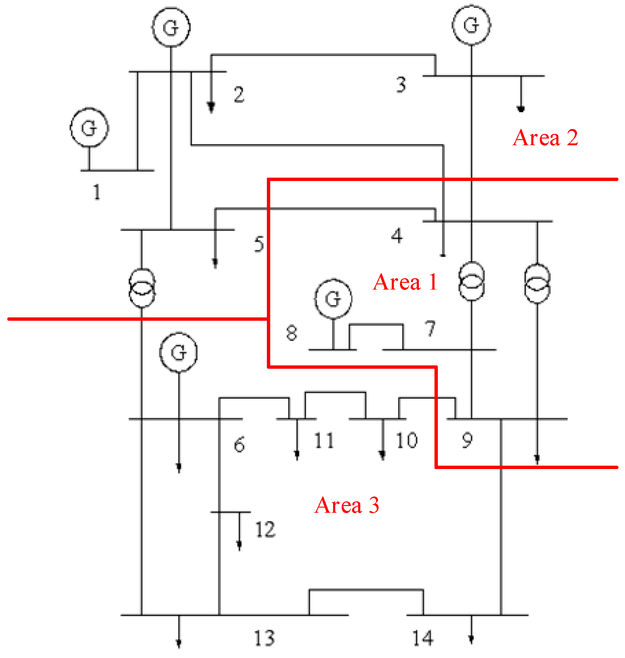
After designing the dynamic partitioning method, the simulation is verified using an IEEE14 node system with the following system topology.

For the nodes, the trend calculation is performed according to the method described in the previous section. The sensitivity matrix S and the electrical distance matrix D are computed. Using the MATLAB 2022b function, hierarchical clustering is then conducted, and the system partition diagram is generated as illustrated in Figure 7.

The power reserve of each partition is as follows in

Table 4. Power reserve for each partition without stations.

Parameter	Area 1	Area 2	Area 3
Active load/MW	42	171.3	45.7
Maximum active power/MW	100	350	100
Active power reserve/%	138.1	104.3	118.8
Reactive load/MW	24.2	29.4	19.9
Maximum reactive power/MW	50	100	40
Reactive power reserve/%	106.6	240.1	101.0

.

The power reserve in each zone is sufficient, with the active reserve distributed evenly. The minimum active reserve level is 104.3%, and the minimum reactive reserve level is 101.0%, indicating that the zoning method is reasonable.

At nodes 2, 10, and 12, EV charging stations are connected for partitioned optimization analysis in various scenarios. The first scenario is in a stable operating normal state, the second scenario is in a state of excessive load or sudden increase in load for EVs, and the third scenario is a high load state in the core work area while the two suburbs are in a normal load state.

(1)

All three power stations are in normal or low-load charging.

Set the charging power of the three power stations to 20 MW (the general power station rarely exceeds this power) and carry out the partition simulation; the partition results are the same as above, and the power reserves of each partition are as follows in

Table 5. Power reserve for each partition when three power stations are in normal or low-load charging.

Parameter	Area 1	Area 2	Area 3
Active load/MW	62	191.3	65.7
Maximum active power/MW	100	350	100
Active power reserve/%	61.29	82.96	52.21
Reactive load/MW	24.2	29.4	19.9
Maximum reactive power/MW	50	100	40
Reactive power reserve/%	106.6	240.1	101.0

.

The power reserves in each zone are relatively sufficient, with a minimum active power reserve of 52.21% and a minimum reactive power reserve of 101.0%. The power system has an adequate stability margin.

The power flow section of the power system before and after the partition is as follows in Figure 8.

Before partitioning, the total voltage fluctuation of the PQ nodes was 0.2594. After partitioning, it decreased to 0.2024. The ratio of these values is 1.2816, indicating a significant improvement in power system stability, with the voltage at each node becoming more consistent.

(2)

A power station is in a high-load state.

The Node 12 electric car charging station is set at a high load of 40 MW, while the other two stations remain at 20 MW, conducting partition simulation and leading to changes in the partition results, as shown in Figure 9.

At this point in time, the power reserves for each subdistrict are as follows in

Table 6. Power reserve for each partition when a power station is in a high-load state.

Parameter	Area 1	Area 2	Area 3
Active load/MW	76.9	191.3	70.8
Maximum active power/MW	100	350	100
Active power reserve/%	30.04	82.96	41.24
Reactive load/MW	29.2	29.4	14.9
Maximum reactive power/MW	50	100	40
Reactive power reserve/%	71.23	240.1	168.5

.

The power reserve is more than sufficient in all subareas, with a minimum active reserve of 30.04% and a minimum reactive reserve of 71.23%, and the power system has sufficient stability margins.

The power flow section of the power system before and after the partition is as follows in Figure 10.

The total voltage fluctuation at PQ nodes is 0.2278 before partitioning and 0.1435 after partitioning. This yields a ratio of 1.5875, demonstrating a substantial improvement in power flow stability within the system, with voltages at each node becoming more stable.

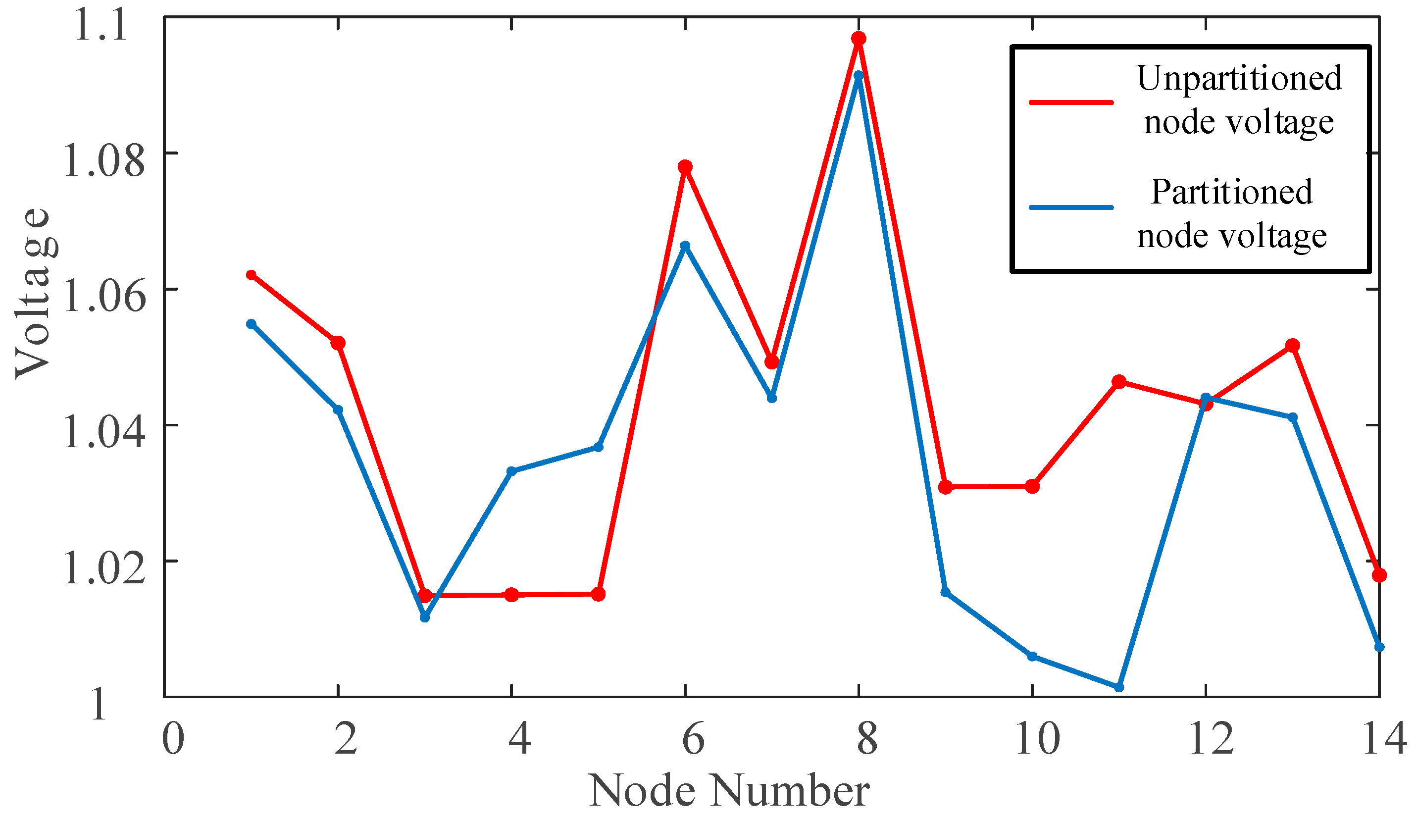
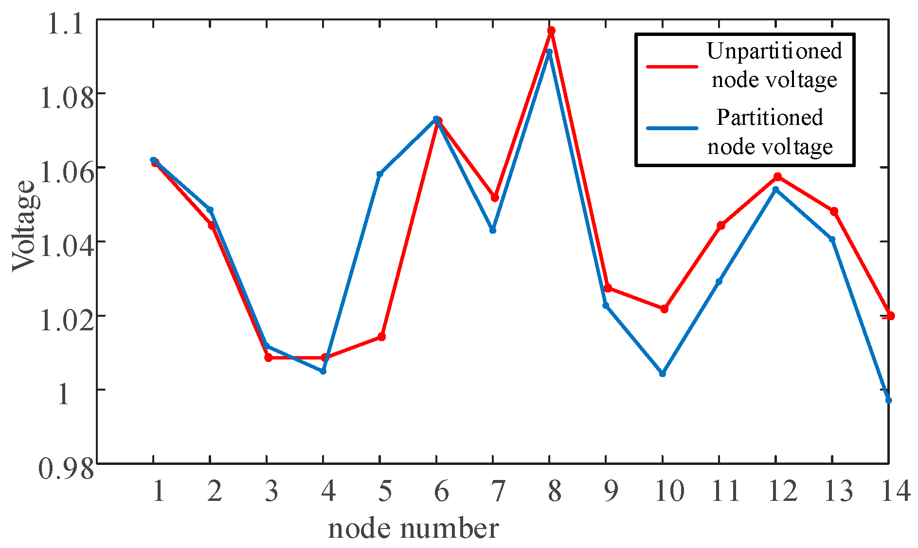
(3)

One partition is under an abnormally high load, one partition power station discharges at low power, and the other partition power station charges at low power.

As shown in the partition results in Figure 11, Node 2’s EV station is under a substantial load of 130 MW, Node 10’s station has a load of 15 MW, and Node 12’s station discharges 5 MW to the grid.

At this time, the power reserve of each partition is as follows in

Table 7. Power reserve for each partition of situation (3).

Parameter	Area 1	Area 2	Area 3
Active load/MW	77.3	253.5	73.2
Maximum active power/MW	100	350	105
Active power reserve/%	29.37	38.07	43.44
Reactive load/MW	12.7	33.3	27.5
Maximum reactive power/MW	50	100	40
Reactive power reserve/%	293.7	200.3	45.45

.

Under such extreme conditions, dynamic partition adjustment ensures that each partition maintains sufficient power reserves within the region, with a minimum active power reserve of 29.37% and a minimum reactive power reserve of 45.45%, thereby meeting the requirements.

The power flow profile of the power system before and after the partition is as follows in Figure 12.

Using MATLAB 2022b, the total voltage fluctuation of the PQ node without partitioning is 0.2997, while after partitioning, it is 0.2429. The ratio of these values is 1.2335, indicating an improvement in the power system’s current and increased voltage stability at each node.

7.2. Simulation Parameter Setting of FM and Peak Shaving Backup Scene

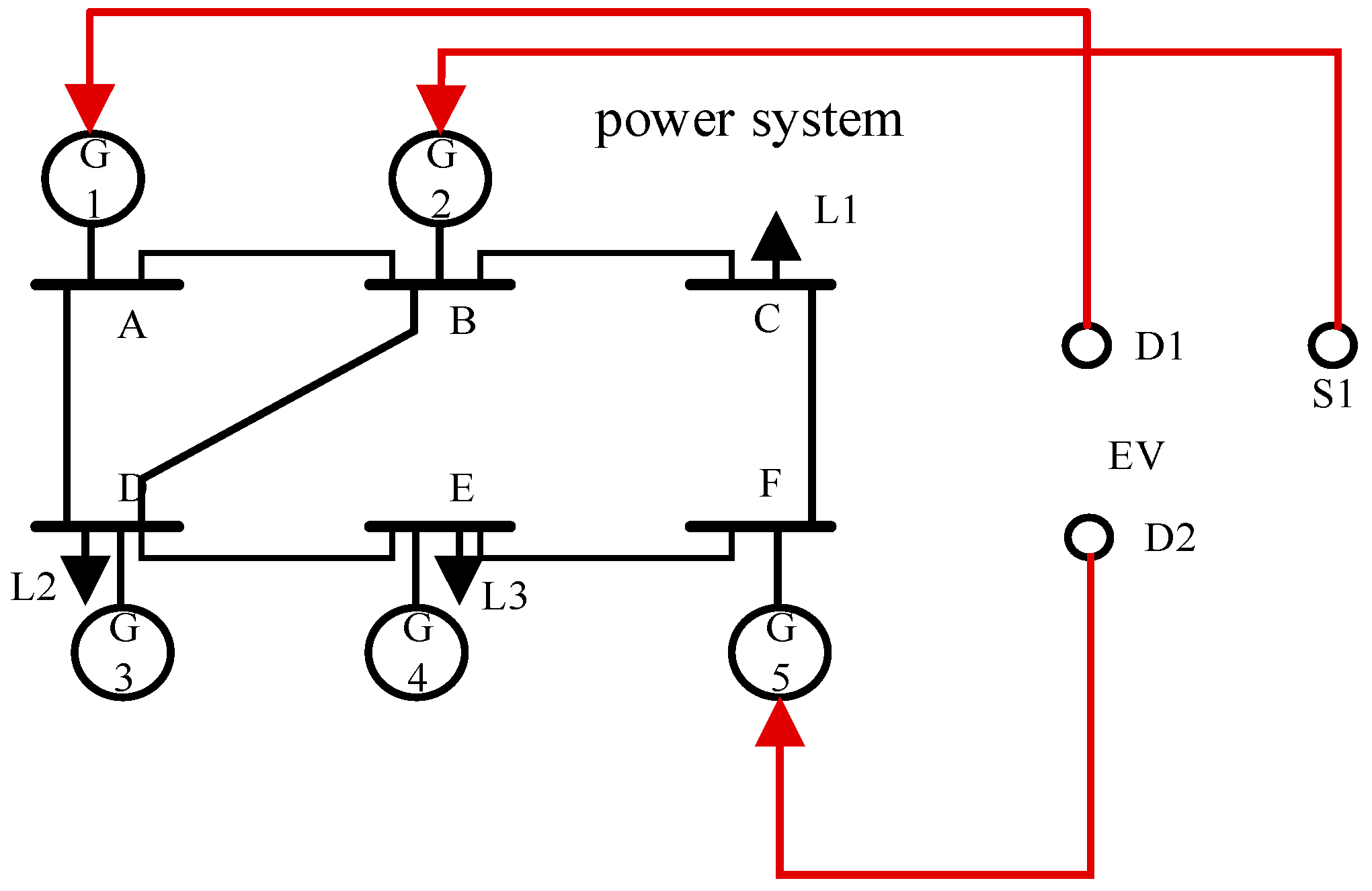
This article conducts a simulation based on data from three EV charging stations provided by Teli Electric Company (Chongqing, China) and power grid data for the city of Chongqing provided by State Grid Chongqing Electric Power Company. The load disturbance model incorporates randomly added disturbances for simulation purposes. The AGC module operates in constant frequency control mode. The system simulation parameters are listed in

Table 8. System simulation parameters.

Parameter	Numerical Value
System reference capacity/MW	100
Benchmark rating/HZ	50
Inertia constant of generator M/s	10
Governor time constant Tg	0.2
Steam turbine time constant T	0.3
Frequency deviation factor β	3
PI parameters	2, 1.6
Load damping coefficient D	1
Frequency bias coefficient R	0.25

, and the system topology diagram is illustrated in Figure 13. Among them, the G node represents the generator node, the D node represents the DC charging station, and the S node represents the AC charging station. The three charging stations on the red line are connected to the generator nodes of the power system.

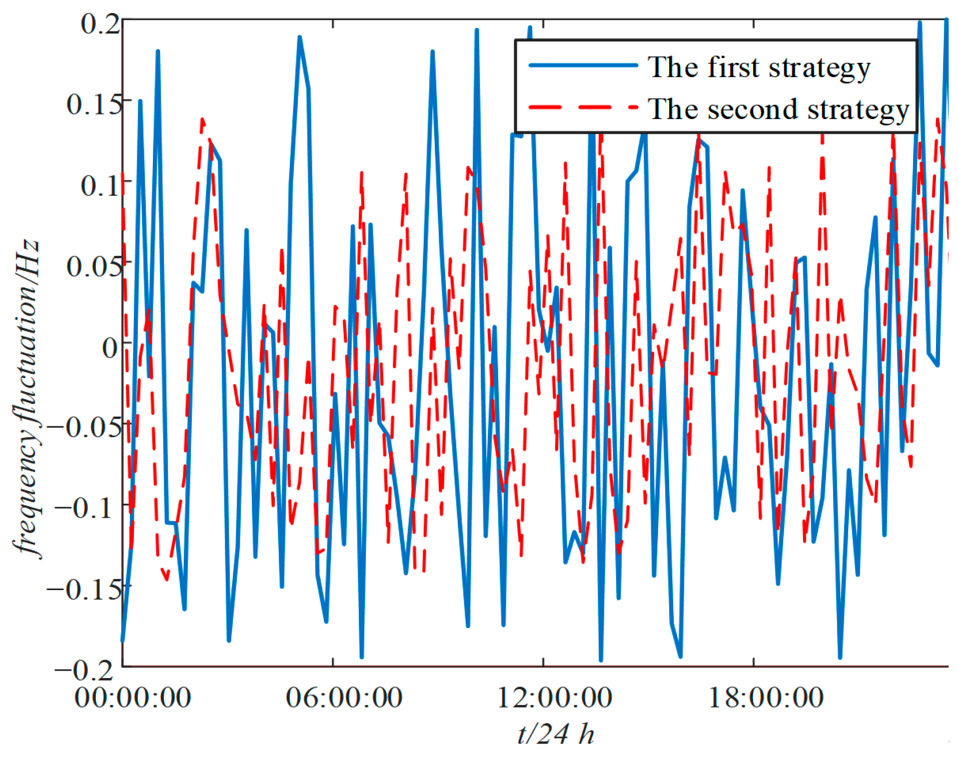
7.3. FM Scene Analysis

This article presents a comparison between the traditional AGC strategy and the two-stage optimized APC strategy introduced within this study, focusing on frequency regulation and load balancing in the power grid. The first approach entails the conventional AGC frequency control method, whereas the second involves the newly proposed two-stage optimized APC frequency control strategy.

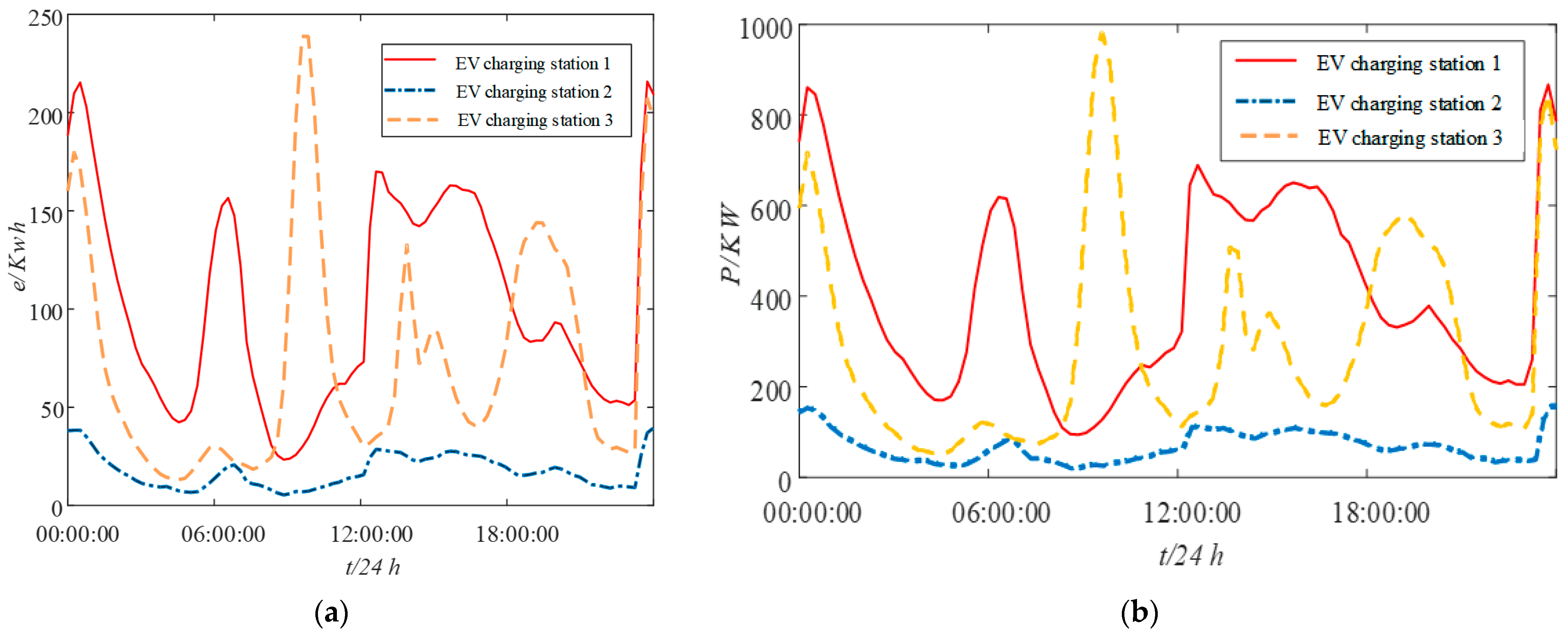
The assessment of the adjustable capacity of the EV load profile at the charging station over the course of one year is represented in Figure 14, Figure 15 and Figure 16.

The output of each unit under the two strategies is illustrated in Figure 15, while the frequency deviation is depicted in Figure 16. The results indicate that the frequency fluctuation of the second strategy is marginally smaller than that of the first strategy. This is because the fluctuation in the output of each unit is not significantly large. Given that the capacity of the current EV load is insufficient for the municipal grid’s FM task, it can only contribute to a portion of the auxiliary FM task.

7.4. Peak Shaving and Standby Scenario Analysis

Perform K-means clustering on the load scenarios of each day within a year, select four typical load scenarios, and conduct daily operation simulation of all units for each month of the year under these four scenarios. Figure 17 shows the typical load curve.

Both the winter load curve and the summer load curve are not very different from each other, and the peak periods of electricity consumption are from 10 to 12 o’clock versus around 18 to 20 o’clock.

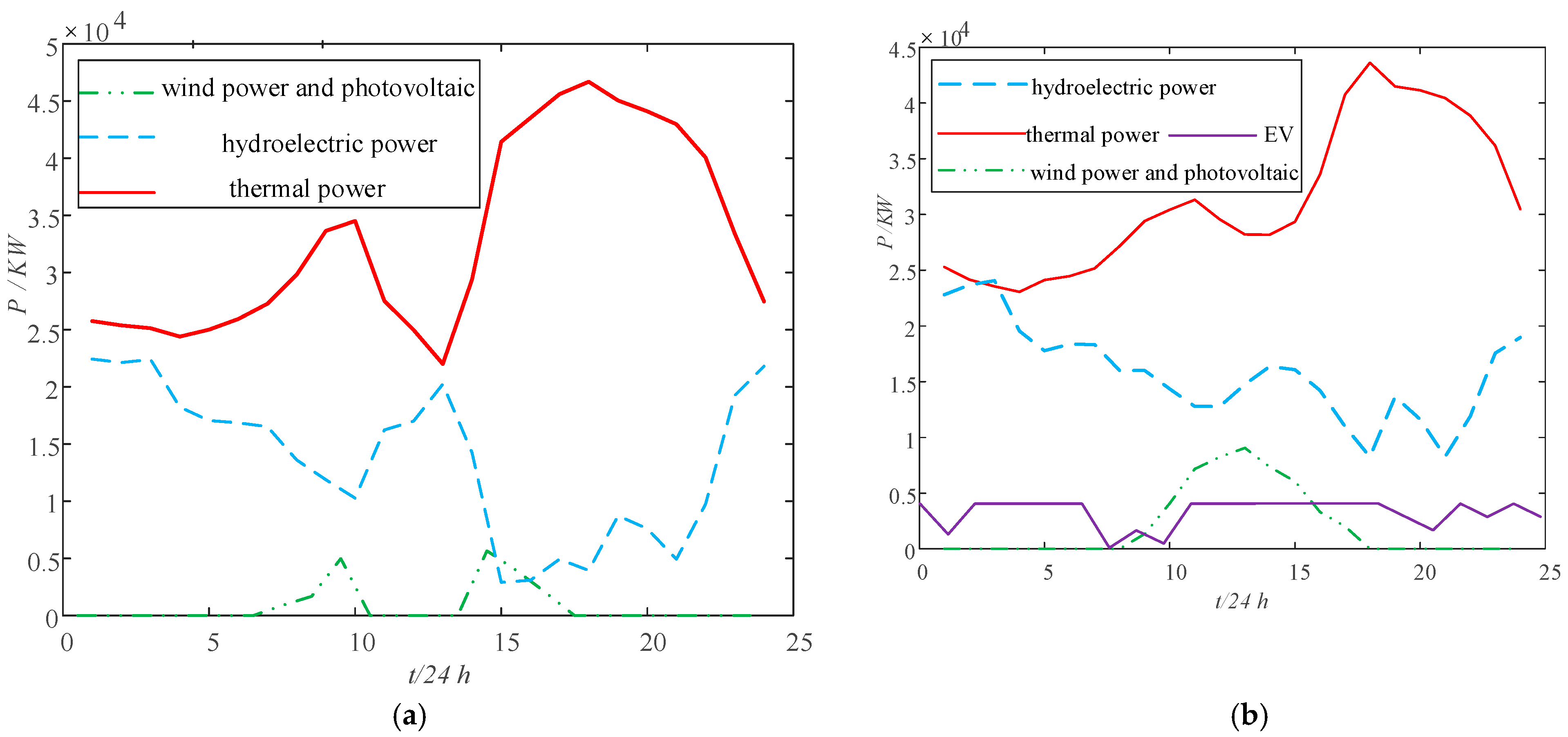
In this section, we conduct a comparative study using two strategies: Strategy 1, which does not introduce EV load peaking, and Strategy 2, which does. Figure 18 presents the daily operating simulation curves for each unit’s output under both strategies, as well as the total EV load output under Strategy 2.

In Strategy 1, the power generation mix primarily consists of photovoltaic and thermal power, with minor contributions from hydroelectricity, wind power, and pumped storage. As shown in the figure, external power delivery and thermal power collectively account for 95% of the output throughout the day, with their output curves aligning with the expected 24 h distribution. PV output occurs between 06:00 and 18:00. Due to the limited number of pumped storage units, cross-regional power transmission plays a significant role in load balancing.

In Strategy 2, thermal power output decreases compared to Strategy 1, with reductions of 1.4% and 6% at two peak points, respectively. Although the magnitude of the EV load is not substantial, the decrease is not particularly pronounced. However, the introduction of EV load for peak shaving backup can alleviate peak shaving pressure on thermal power units, thereby contributing to the achievement of dual carbon goals.

8. Conclusions

The traditional automatic generation control (AGC) method relies on the load regulation of large generating units. While it can effectively control grid frequency, its regulation capability and accuracy diminish with the increasing integration of distributed loads such as electric vehicles. In contrast, the EV-based load regulation method proposed in this paper offers real-time dynamic load adjustment with high flexibility and precise regulation. The optimal interaction between EV loads and the grid can be achieved by adjusting charging and discharging power, providing reserve capacity to the grid, and participating in peak shaving and FM. This article explores the integration of EV loads into peak shaving and frequency regulation services within the grid, achieving the following:

(1)

The spare capacity of EV loads is constrained by factors such as user travel demand and battery degradation, limiting unrestricted dispatch. The article first comprehensively considers constraints such as charging station power limits and battery charge levels, proposing a method to assess the real-time adjustable capacity of EVs on a large scale. This method utilizes real-time EV data, evaluates the upper limit of charging and discharging power using historical charging station data, determines the maximum allowable charging power based on battery level constraints, and combines current power levels to evaluate the capacity for the upward and downward adjustment of EVs within a scheduling period.

(2)

In the context of a large number of connected EVs, a dynamic partition model of the power system with EV participation was designed based on the existing power system dynamic partition methods. The model was validated using the IEEE14 node system, resulting in three partitions. Simulation results under three scenarios indicate that partitioning can improve total voltage fluctuation of PQ nodes by 28.16%, 58.75%, and 23.35%, respectively, demonstrating that partitioning can regulate power distribution, improve grid flow, and respond to various situations.

(3)

Expanding AGC to APC, the APC algorithm was used to conduct rolling optimization of EV load control commands, achieving precise control of EV loads. To fully exploit the frequency regulation capabilities of EV loads and reduce operating costs, while considering the demand for frequency regulation time, a two-stage optimization model for EV load participation in grid frequency regulation is proposed. The two-stage optimization APC strategy improves maximum frequency deviation by approximately 25% compared to the traditional AGC strategy.

(4)

In the peak shaving standby scenario, typical load scenarios were extracted. Compared to traditional AGC frequency control strategies, significant reductions in peak power generation at thermal power plants were achieved, with reductions of approximately 15% and 10% during the morning and evening peaks, respectively.

This article evaluates the dispatchable capacity of EVs in specific scenarios and models the participation of EVs in secondary frequency regulation and peak shaving scenarios; however, the model still lacks consideration of indicators such as charging station power ramp rates and response times. This may result in the model not accurately reflecting the transient regulation capability of EV loads in real scenarios, especially in frequency regulation scenarios that require a fast response, and the actual results may deviate from the theoretical expectations. Additionally, when the EV load peaking capacity is insufficient, the model does not propose a supplemental strategy for load-side standby capacity, nor does it design a co-dispatch mechanism between generation-side standby units and the load side. This unidirectional regulation model may lead to a reserve capacity gap in the system under extreme operating conditions, limiting the robustness of the strategy. Furthermore, due to the relatively low power level of EV loads in the case study data from the Chongqing power system, the case study verification results are not particularly significant. Future work will focus on improving the mathematical model, optimizing the control strategy for EV loads, and further refining the case study analysis.

References

- Chen, J.; Luo, G. “Synergistic Interaction Between Source, Network, Load and Storage” to Accelerate Energy Efficiency Improvement; China Power Enterprise Management: Beijing, China, 2021; pp. 22–23. [Google Scholar]
- Ministry of Transport, Central Publicity Department, National Development and Reform Commission. Twelve ministries and commissions release “Green Travel Action Plan (2019–2022)”. People’s Bus 2019, 25–27. [Google Scholar] [CrossRef]
- Zhang, T. China’s New Energy Vehicle Fleet Reaches 7.84 Million by the End of 2021. Chinese Government Website, 12 January 2022. Available online: https://www.gov.cn/xinwen/2022-01/12/content_5667734.htm (accessed on 1 March 2025).
- Cavus, M.; Ayan, H.; Bell, M.; Oyebamiji, O.K.; Dissanayake, D. Deep charge-fusion model: Advanced hybrid modelling for predicting electric vehicle charging patterns with socio-demographic considerations. Int. J. Transp. Sci. Technol. 2025; in press. [Google Scholar] [CrossRef]
- Nikoobakht, A.; Aghaei, J.; Shafie-khah, M.; Catalão, J.P. Co-operation of electricity and natural gas systems including electric vehicles and variable renewable energy sources based on a continuous-time model approach. Energy 2020, 200, 117484. [Google Scholar] [CrossRef]
- Ge, L.; Wang, Q.; Wang, M. Multi-stage operation strategy of electric vehicle aggregator participating in energy and frequency regulation markets considering charging and discharging incentive mechanisms. Electr. Power Autom. Equip. 2024, 44, 176–184. [Google Scholar]
- Wang, Y.; Mao, M.; Yang, C. Modeling for Large-scale EV Aggregated Dispatchable Capacity Considering Multi-scenario Ancillary Services. Autom. Electr. Power Syst. 2024, 48, 103–115. [Google Scholar]
- Li, J.; Ai, X.; Hu, J. Modeling and control strategies for electric vehicle participation in grid secondary frequency regulation. Power Grid Technol. 2019, 43, 495–503. [Google Scholar]
- Liu, Q.; Lu, S. Charging and discharging control strategy based on virtual synchronous machine for electrical vehicles participating in frequency regulation of microgrid. Autom. Electr. Power Syst. 2018, 42, 171–179. [Google Scholar]
- Gao, S.; Dai, R. Charging control strategy for electric vehicle cluster participating in frequency regulation ancillary service mark. Autom. Electr. Power Syst. 2023, 47, 60–67. [Google Scholar]
- Yu, Y.; Zhang, R.; Lu, W.; Mi, Z.; Cai, X. Auxiliary Frequency Regulation Control Strategy of Aggregated Electric Vehicles Based on Lyapunov-Based Economic Model Predictive Control. Trans. China Electrotech. Soc. 2022, 37, 6025–6040. [Google Scholar]
- Zhang, C.; Zhang, X.; Xia, J. Research on estimation of electric vehicles real-time schedulable capacity. Power Syst. Prot. Control. 2015, 43, 99–106. [Google Scholar]
- Yang, Z.; Shi, Y.; Li, P.; Pan, K.; Li, G.; Li, X.; Yao, S.; Zhang, D. Application of Principal Component Analysis (PCA) to the Evaluation and Screening of Multiactivity Fungi. J. Ocean. Univ. China 2022, 21, 763–772. [Google Scholar] [CrossRef] [PubMed]
- Ji, Y.; Chen, X.; Xue, Y.; He, P.; Wang, J.; Guo, L. Voltage and reactive power partitioning of distribution network considering the temporal information of “source-load”. J. Electr. Power Sci. Technol. 2022, 37, 45–56. [Google Scholar]
- Amaral, T.G.; Pires, V.F.; Pires, A.J. Fault Detection in PV Tracking Systems Using an Image Processing Algorithm Based on PCA. Energies 2021, 14, 7278. [Google Scholar] [CrossRef]
- Chen, X.; Li, L.; Liu, R.; Yang, B.; Deng, Z.; Li, Z. Fault diagnosis method of wind turbine pitch angle based on PCA-KNN fusion algorithm. China Electr. Power 2021, 54, 190–198. [Google Scholar]
- Rodriguez, A.; Laio, A. Machine learning. Clustering by fast search and find of density peaks. Science (Am. Assoc. Adv. Sci.) 2014, 344, 1492–1496. [Google Scholar] [CrossRef] [PubMed]
- Shu, X.; Zhang, L.; Sun, Y.; Tang, J. Host-Parasite: Graph LSTM-in-LSTM for Group Activity Recognition. IEEE Trans. Neural Netw. Learn. Syst. 2021, 32, 663–674. [Google Scholar] [CrossRef] [PubMed]
- Yang, Y.; Wang, Y.; Wei, Y. Adaptive Density Peak Clustering for Determinging Cluster Center. In Proceedings of the 2019 15th International Conference on Computational Intelligence and Security (CIS), Macao, China, 13–16 December 2019; pp. 182–186. [Google Scholar]
- Jing, S.; Hu, C.; Wang, C.; Zhou, G.; Yu, J. Vehicle Face Detection Based on Cascaded Convolutional Neural Networks. In Proceedings of the 2019 Chinese Automation Congress (CAC), Hangzhou, China, 22–24 November 2019; pp. 5149–5152. [Google Scholar]
- Xu, Y.; Yan, X. Dynamic Partitioning Real-Time Reactive Power Optimization Method for Distribution Network with Renewable Distributed Generators Participating in Regulation. Mod. Electr. Power 2020, 37, 42–51. [Google Scholar]
- Guo, Q.; Sun, H.; Zhang, B.; Wu, W. Reactive Voltage Partitioning Based on Cluster Analysis of Reactive Source Control Space. Autom. Electr. Power Syst. 2005, 29, 36–40+54. [Google Scholar]
- Chen, H.; Hu, J.; Yuan, H.; Zhou, H.; Luo, K. Cluster electric vehicles taking into account distribution network congestion participate in secondary frequency modulation method research. Electr. Power 2021, 54, 162–169. [Google Scholar]
- Wu, Q.; Song, X.; Zhang, J.; Yu, H.; Huang, J.; Dai, H.; Luo, H. Study on Self-adaptation Comprehensive Strategy of Battery Energy Storage in Primary Frequency Regulation of Power Grid. Power Grid Technol. 2020, 44, 3829–3836. [Google Scholar]
Figure 1.
EV single adjustable capacity.
Figure 2.
Block diagram of the procedure for adjustable capability assessment of EV load.
Figure 3.
Block diagram of dynamic partitioning.
Figure 4.
Block diagram of the control logic of the APC.
Figure 5.
Block diagram of the APC program.
Figure 6.
Schematic diagram of the optimization model for the load FM module.
Figure 7.
IEEE14 node system allocated area diagram without stations or when all stations are in normal charging.
Figure 8.
Power system trend cross-section when three power stations are in normal or low-load charging.
Figure 9.
IEEE14 node system allocated area diagram when a power station is in a high-load state.
Figure 10.
Power system trend cross-section when a power station is in a high-load state.
Figure 11.
IEEE14 node system allocated area diagram of situation (3).
Figure 12.
Power system trend cross-section of situation (3).
Figure 13.
System topology.
Figure 14.
EV load’s adjustable capacity and adjustable power diagram. (a) Adjustable capacity. (b) Adjustable power.
Figure 15.
Output graph for each unit. (a) without EV. (b) with EV.
Figure 16.
Frequency deviation.
Figure 17.
Typical load curve.
Figure 18.
Daily operating simulation graphs for each unit’s output. (a) Strategy 1. (b) Strategy 2.