Article

Research on Calibration Method of Triaxial Magnetometer Based on Improved PSO-Ellipsoid Fitting Algorithm

1
School of Automation, Jiangsu University of Science and Technology, Zhenjiang 212100, China
2
National Key Laboratory of Transient Physics, Nanjing University of Science and Technology, Nanjing 210094, China
3
Huaihai Industries Group Co., Ltd., Changzhi 046012, China
*
Author to whom correspondence should be addressed.
Electronics 2025, 14(9), 1778; https://doi.org/10.3390/electronics14091778
Submission received: 26 March 2025 / Revised: 23 April 2025 / Accepted: 25 April 2025 / Published: 27 April 2025
(This article belongs to the Special Issue Advancements in Connected and Autonomous Vehicles)

Abstract

:
To address the measurement accuracy degradation of triaxial magnetometers caused by manufacturing errors and environmental interference, and the limited robustness of traditional calibration methods, this study proposes a Dynamic Hierarchical Elite-guided Particle Swarm Optimization (DHEPSO)-based ellipsoid fitting algorithm. First, an error model for the triaxial magnetometers is established. Next, the DHEPSO algorithm is utilized to fit the ellipsoid parameters by integrating a dynamic hierarchical mechanism, elite guidance strategy, and adaptive inertia weight adjustment, thereby balancing global exploration and local exploitation to efficiently optimize the parameters. Finally, error compensation and precise calibration are achieved using the optimized parameters. The simulation results show that, compared to the Least Squares Method (LSM), it reduces the absolute distance between the simulated data and the ellipsoid by 63.10% and the post-calibration total magnetic field intensity standard deviation by 60% under outlier interference. Against the traditional PSO, TSLPSO, MPSO, and AWPSO, DHEPSO achieves total distance reductions of 48.52%, 47.74%, 56.71%, and 33.09%, respectively, with faster convergence. The statistical analysis of 60 trials confirms DHEPSO’s stability, exhibiting lower median error and interquartile range. The results validate DHEPSO’s high precision and robustness in high-noise environments, offering theoretical support for engineering applications.

1. Introduction

Connected and Automated Vehicles (CAVs) leverage multi-source sensor fusion and real-time decision-making to achieve precise path planning and coordinated control in complex traffic scenarios, positioning them as critical technological enablers for improving traffic efficiency, reducing energy consumption, and minimizing accident rates [1,2]. To realize these objectives, CAVs rely on high-precision sensors to acquire key information such as vehicle body orientation, ensuring the reliability and safety of control algorithms. Among these sensors, the triaxial magnetometers—passive, all-weather magnetic field measurement units—are widely utilized in vehicle attitude estimation and geomagnetic navigation. Their measurement accuracy directly impacts vehicle positioning precision and the robustness of decision-making systems.
However, the triaxial magnetometers face significant technical challenges in practical engineering applications—their measurements are susceptible to dual influences from manufacturing imperfections and environmental interference, resulting in systematic deviations in the output data. Specifically, measurement errors can be categorized into two major classes:
  • Sensor fabrication errors, including sensitivity errors, non-orthogonality errors, and zero-offset errors caused by material properties and machining precision limitations;
  • Environmental interference errors, primarily stemming from hard-iron interference generated by the vehicle’s ferromagnetic materials and soft-iron interference arising from the magnetization of surrounding magnetic substances under external magnetic fields [3].
If uncalibrated, such errors may introduce deviations in vehicle attitude estimation, thereby threatening the safety margins of cooperative driving and even leading to control algorithm failures. Consequently, developing high-precision, robust magnetometer calibration methods constitute a foundational prerequisite for ensuring reliable interaction between CAV perception systems and infrastructure, as well as compliance with autonomous driving safety verification standards.
In traditional magnetometer calibration methods, the Least Squares Method (LSM) and ellipsoid fitting techniques have been widely adopted. Fang et al. [4], Zhi et al. [5], and Peng et al. [6], respectively, introduced the LSM to estimate error parameters based on multi-position measurements, ellipsoid fitting, and functional modeling. However, the LSM is known to be sensitive to outliers, as large residuals are significantly amplified during the squaring operation, potentially leading to model deviation and biased parameter estimation. Furthermore, such methods typically rely on matrix inversion; when the design matrix exhibits a high condition number, noise and outliers may amplify numerical errors, rendering the solution highly sensitive to data perturbations and thus reducing calibration accuracy. To enhance robustness, Li et al. [7] proposed an improved LSM-based ellipsoid fitting method utilizing Random Sample Consensus (RANSAC). Although this method improves resilience to the outliers, the randomness inherent in RANSAC can still be affected by the noise, compromising model selection accuracy and thereby reducing calibration precision. Overall, the traditional methods lack sufficient noise resistance and robustness, limiting their effectiveness in complex calibration scenarios.
In recent years, intelligent optimization algorithms have been extensively applied to magnetometer error compensation tasks, demonstrating strong parameter estimation capabilities and system robustness. Some studies focus on enhancing the synergy between global search and local fitting. For instance, Gong et al. [8] employed the Artificial Fish Swarm Algorithm (AFSA) to jointly estimate intrinsic errors and external disturbances; Yang et al. [9] combined the Dragonfly Algorithm with the Levenberg–Marquardt (LM) method to balance global exploration and local convergence, and Li et al. [10] proposed a staged Longhorn Beetle Antennae Search strategy to achieve a trade-off between convergence speed and estimation accuracy. Meanwhile, other studies aim to improve model robustness by mitigating sensitivity to initial values and strong parameter correlations. Pang et al. [11] applied Genetic Algorithms to reduce high inter-parameter correlation, while Pang et al. [12] adopted Differential Evolution to decrease sensitivity to initial values. In addition, Huang et al. [13] introduced an immune adaptive Particle Swarm Optimization (PSO) algorithm to enhance anti-interference capability, and Wu et al. [14] as well as Lei et al. [15] employed a stretching strategy and an improved Grey Wolf Optimizer, respectively, to enhance adaptability in complex parameter spaces. Chafi et al. [16] proposed a two-stage framework integrating LSM with PSO, achieving fast and stable convergence within constrained solution spaces. Although these methods have shown promising results across various experimental scenarios, challenges such as insufficient robustness and unstable convergence remain in highly dynamic and strongly disturbed magnetic environments.
To enhance nonlinear modeling and dynamic adaptability, several studies have explored deep learning approaches. Nerrise et al. [17] integrates physical modeling with liquid time-constant networks to separate interference from geomagnetic signals. Tian et al. [18] uses a model-free MLP-based approach to learn nonlinear sensor mappings. Cowart III et al. [19] incorporates higher-order polynomial models into neural networks with embedded physical constraints, addressing complex nonlinearities and rotation ambiguities. Despite their effectiveness, deep learning models still face challenges in interpretability and computational cost, limiting their use on resource-constrained platforms.
In addition to algorithmic advances, some studies focus on improving the efficiency and feasibility of practical magnetometer calibration. Zikmund et al. [20] combines Helmholtz coils and Overhauser magnetometers to achieve field calibration through nonlinear optimization. Tabatabaei et al. [21] developed an efficient calibration algorithm based on nine independent measurements. Ye et al. [22] introduced a compensation strategy for large UAVs by integrating INS and GPS data. Yu et al. [23] presented an inclination-based calibration method for wearable sensors.
To address the aforementioned challenges, this study proposes an ellipsoid fitting algorithm based on the Dynamic Hierarchical Elite-guided Particle Swarm Optimization (DHEPSO) for a high-precision calibration of the triaxial magnetometers in complex environments. The methodology operates in three sequential phases: First, DHEPSO-based ellipsoid parameter fitting overcomes the limitations of the conventional least squares methods—specifically weak noise resistance and susceptibility to outlier-induced fitting deviations—by integrating the physical constraints derived from the geometric ellipsoid model to align with the spatial distribution patterns of the geomagnetic vectors; second, an error calibration model is constructed using the optimized ellipsoid parameters; finally, raw geomagnetic data are systematically calibrated through the derived model, ensuring robustness against environmental disturbances while maintaining computational efficiency.
The rest of the paper is organized as follows. Section 2 establishes the error model of the triaxial magnetometer and elaborates on the fundamental principles of the conventional ellipsoid fitting algorithm. Section 3 presents the proposed DHEPSO-based ellipsoid fitting algorithm, detailing its improvement strategies. Section 4 provides experimental validation and comparative analysis. Conclusions are given in Section 5.

2. Error Model and Ellipsoid Fitting Algorithm

2.1. Error Model of Triaxial Magnetometer

To address manufacturing errors and environmental interference errors in the triaxial magnetometers, the relationship between their measured data and actual data can be represented by Equation (1) [24]:
H m = K s i K n K s H r + H h + H 0
where H m is the actual measured value of the triaxial magnetometer, H r is the ideal output value, K s i is the sensitivity error matrix, K n is the non-orthogonality error matrix, K s is the soft-iron interference matrix, H h is the hard-iron interference vector, and H 0 is the zero-offset error vector.
By combining the error terms, Equation (1) can be further simplified as:
H m = K H r + H
where K = K s i K n K s , H = K s i K n H h + H 0 . Based on Equation (2), the magnetometer error compensation model is derived as:
H r = K 1 H m H
Under ideal conditions, the total intensity of the geomagnetic field measured by a triaxial magnetometer is a constant value H b , and the measured magnetic data lies on a spherical surface with radius H b [25]. Using the error compensation model defined in Equation (3), the total geomagnetic field intensity can be expressed as:
H b 2 = H r T H r = H m H T K 1 T K 1 H m H
that is:
H m H T K 1 T K 1 H b 2 H m H = 1

2.2. Ellipsoid Fitting Algorithm

In practical measurements, under the influence of measurement errors, the output data of the triaxial magnetometers will distribute on an ellipsoidal surface with a deviated center. A deterministic mathematical mapping relationship exists between the ellipsoid parameters and the magnetometer error model coefficients, enabling the derivation of geomagnetic error correction parameters through ellipsoid parameter solving [26].
As a specific form of quadric surfaces, the standard equation of an ellipsoid can be expressed as:
F ξ , z = ξ T z = a x 2 + b y 2 + c z 2 + 2 d x y + 2 e x z + 2 f y z + 2 p x + 2 q y + 2 r z + g = 0
where z = x 2 , y 2 , z 2 , 2 x y , 2 x z , 2 y z , 2 x , 2 y , 2 z , 1 T represents the composite vector formed by measured triaxial geomagnetic data and ξ = a , b , c , d , e , f , p , q , r , g T represents the ellipsoid parameter vector.
An ellipsoid fitting model is constructed based on the least squares criterion [27]:
min ξ F ξ , z 2 = min ξ ξ T D T D ξ
where D is the measurement data matrix defined as:
D = x 1 2 y 1 2 z 1 2 2 x 1 y 1 2 x 1 z 1 2 y 1 z 1 2 x 1 2 y 1 2 z 1 1 x 2 2 y 2 2 z 2 2 2 x 2 y 2 2 x 2 z 2 2 y 2 z 2 2 x 2 2 y 2 2 z 2 1 x n 2 y n 2 z n 2 2 x n y n 2 x n z n 2 y n z n 2 x n 2 y n 2 z n 1
Rewriting the ellipsoid Equation (6) in vector form yields:
X X 0 T A X X 0 = 1
where A = a d e d b f e f c is the ellipsoid shape parameter matrix, X 0 = A 1 p q r represents the ellipsoid center coordinates.
By combining Equations (5) and (9), the parameter transformation relationship is derived:
K 1 T K 1 H b 2 = G T G = A H = X 0
where G is an upper triangular matrix. Since A satisfies symmetric positive definiteness, the error correction matrix K 1 can be calculated via Cholesky decomposition of A [28].
K 1 = H b G
Once the error correction matrix K 1 and bias vector H are obtained, magnetometer measurement errors can be compensated through Equation (3).
Figure 1 illustrates the complete computational workflow of the ellipsoid fitting algorithm.

3. Ellipsoid Fitting Algorithm Based on Dynamic Hierarchical Elite-Guided Particle Swarm Optimization

3.1. Conventional PSO Algorithm

The Particle Swarm Optimization (PSO) algorithm is a metaheuristic optimization method grounded in swarm intelligence, whose design is inspired by the spatial search mechanisms observed in bird flock foraging behaviors [29]. Within this algorithmic framework, each particle represents a candidate solution in the solution space, with its motion state jointly defined by a position vector x and a velocity vector v . Particles dynamically adjust their velocity vectors by integrating information from their individual historical optimal position p b e s t and the swarm’s global optimal position g b e s t , enabling progressive convergence toward the global optimum [30,31]. The velocity and position update equations for the standard PSO algorithm are expressed as:
v i t + 1 = ω v i t + c 1 r 1 p b e s t i t x i t + c 2 r 2 g b e s t t x i t
x i t + 1 = x i t + v i t + i
where v i t and x i t denote the velocity vector and position vector of the i - th particle at the k - th iteration, respectively; ω represents the inertia weight, controlling the retention degree of particle motion inertia; c 1 and c 2 are acceleration factors that regulate the contribution weights of individual cognition and social cognition, respectively; p b e s t i t indicates the historical optimal position of the i - th particle up to the k - th iteration; g b e s t t denotes the global optimal position of the entire population up to the k - th iteration; r 1 , r 2 U 0 , 1 are uniformly distributed random variables.

3.2. Enhancement Strategies for Dynamic Hierarchical Elite-Guided Particle Swarm Optimization

In the particle swarm optimization process, exploration of the solution space and exploitation of potential solutions constitute two critical strategies. Achieving a balance between these strategies is essential for efficiently locating the global optimum—ensuring comprehensive exploration while effectively exploiting promising regions. However, conventional PSO algorithms often fail to maintain this equilibrium, exhibiting tendencies toward premature convergence to local optima and consequent performance limitations. To address this, this study proposes the Dynamic Hierarchical Elite-Guided Particle Swarm Optimization (DHEPSO) algorithm, which incorporates three pivotal enhancement strategies: (1) the dynamic hierarchical mechanism: elite and ordinary particles are dynamically classified by comprehensively evaluating particle fitness and solution space distribution density; (2) the elite guidance strategy: differentiated update rules are implemented to dynamically balance exploitation and exploration; (3) adaptive inertia weight adjustment: a nonlinear time-varying inertia weight function is employed to mitigate premature convergence.

3.2.1. Dynamic Hierarchical Mechanism

The dynamic hierarchical mechanism categorizes the particle swarm into elite and ordinary layers through a comprehensive evaluation integrating fitness and crowding distance, as formalized in Equation (14). The stratification criterion, combining fitness and crowding distance, ensures that elite particles not only exhibit superior fitness but also maintain broader spatial distribution in the solution space, preventing excessive clustering in local regions. This preserves population diversity and effectively mitigates premature convergence or entrapment in local optima.
E l i t e = argmax 1 j E s i z e f i d i N o r m a l = argmax E s i z e < j N P f i d i
where E l i t e and N o r m a l denote elite and ordinary particle sets, respectively, E s i z e represents the number of elite particles, argmax f i d i sorts particles by the product of fitness value f i and crowding distance d i .
d i is calculated as follows:
d i = f i + 1 f i 1 f max f m i n
The proportion of elite particles is dynamically adjusted based on population diversity to flexibly balance exploration and exploitation across optimization phases. When population diversity decreases, increasing the proportion of ordinary particles enhances exploration capability, preventing local optima stagnation. Conversely, higher diversity triggers an expanded elite layer, intensifying exploitation in promising regions. This dual adaptation ensures robust and efficient convergence in complex search spaces. The elite proportion is governed by,
E s i z e = r min + r max r min d m e a n d min d max d min
where r min and r max are the minimum and maximum elite proportion, respectively, d min and d max define the allowable crowding distance range, and d m e a n denotes the average crowding distance.

3.2.2. Elite Guidance Strategy

Building upon the hierarchical mechanism, differentiated update strategies are adopted for particles across layers. The elite particles focus on intensive exploitation of high-fitness regions, progressively approaching the global optimum through independent exploration, while the ordinary particles distribute across potential solution subspaces under the elite guidance, assisting in search processes and maintaining population diversity. This framework achieves dynamic equilibrium between exploitation and exploration, facilitating rapid global optimum identification.
  • Elite Layer
The elite layer particles represent the optimal solution set within the search space, with their primary task being deep exploitation of high-fitness regions. The update rules for the elite particles prioritize independent exploration, enhancing their capacity to probe optimal solution subspaces through dual guidance from individual and global historical optima. The velocity and position update rules are formulated as follows:
v i t + 1 = w v i t + c 1 e r 1 p b e s t i t x i t + c 2 e r 2 g b e s t t x i t x i t + 1 = x i t + v i t + 1
where c 1 e and c 2 e denote the individual learning factor and swarm learning factor for the elite layer, respectively.
  • Ordinary Layer
The ordinary particles are primarily responsible for maintaining population diversity and exploring potential regions. Their update rules incorporate an elite guidance term, enabling the ordinary particles to aggregate toward potential solution regions explored by the elite particles while conducting auxiliary searches within these regions. The velocity and position update rules for the ordinary particles are as follows:
v i t + 1 = w v i t + c 1 n r 1 p b e s t i t x i t + c 2 n r 2 g b e s t i t x i t + c 3 n r 3 e l i t e g u i d e x i t + 1 = x i t + v i t + 1
where c 1 n and c 2 n denote the individual and swarm learning factors for the ordinary layer, c 3 n represents the learning factor for the elite guidance term, and e l i t e g u i d e is the elite guidance term, defined as the average positional deviation between the ordinary particle and a randomly selected subset of elite particles:
e l i t e g u i d e = 1 k j ε k x j x i
where ε k denotes a set of k elite particles randomly selected from the elite layer, with k set to 20% of the elite population size in this study.

3.2.3. Adaptive Inertia Weight Adjustment

In PSO algorithms, higher inertia weights enable particles to maintain greater velocities, increasing the probability of movement to new neighborhoods and thereby enhancing exploration capability. Conversely, lower inertia weights reduce particle velocities, focusing their efforts on the exploitation and refinement of current regions to strengthen local optimization. By dynamically adjusting the inertia weight, a balance between exploration and exploitation can be achieved, improving PSO performance across different search phases. This study adopts a nonlinear time-varying inertia weight proposed by Yang et al. [32], which accelerates swarm search and promotes faster convergence while maintaining exploration–exploitation equilibrium. The inertia weight adjustment formula is as follows:
ω = ω max ω max ω min t T α
where α controls the decay rate, with α set to 1 / π 2 in this study, ω min and ω max denote the minimum and maximum values of the inertia weight, t represents the current iteration count, and T indicates the maximum number of iterations.

3.2.4. Ellipsoid Constraints

To ensure the optimized surface satisfies the ellipsoid geometric properties, a constraint validation and correction mechanism for ellipsoid conditions is embedded within the DHEPSO algorithm. The rotational invariants are defined as constraint terms [33], as shown in Equation (21):
I 1 = a + b + c ; I 2 = a b + b c + a c d 2 e 2 f 2 ; I 3 = det a , d , e ; d , b , f ; e , f , c ; I 4 = det a , d , e , p ; d , b , f , q ; e , f , c , r ; p , q , r , g ;
The necessary and sufficient conditions for a quadric surface to represent an ellipsoid are formulated as follows:
I 1 0 & I 2 > 0 & I 1 × I 3 > 0 & I 4 < 0
During DHEPSO iterations, each particle position undergoes ellipsoid constraint validation:
  • If Equation (22) is satisfied, the current solution is retained;
  • If Equation (22) is violated, the particle position is stochastically perturbed with minor amplitude;
  • This mechanism guarantees precise ellipsoid model fitting via DHEPSO;
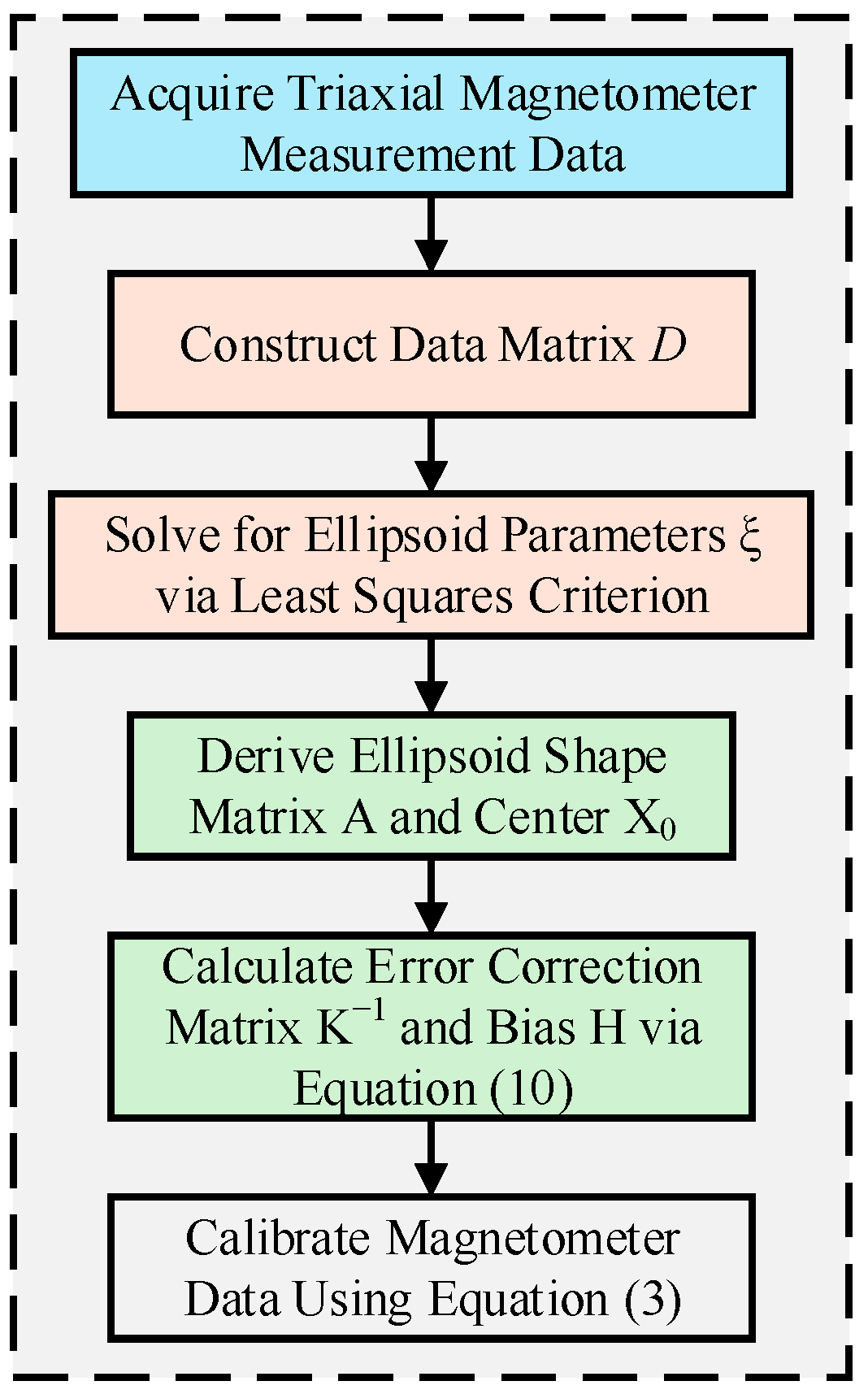
  • Figure 2 illustrates the complete workflow of the DHEPSO algorithm.

3.3. Ellipsoid Fitting Algorithm Based on DHEPSO

Conventional ellipsoid fitting methods employ the least squares to fit data points to an ellipsoid model. However, their sensitivity to noise and outliers often induces significant fitting deviations. To address this limitation, this study proposes a DHEPSO-based ellipsoid fitting algorithm. By simulating the swarm intelligence cooperative search mechanism, the algorithm achieves the global optimal parameter estimation within the feasible solution space, significantly enhancing fitting robustness and model adaptability in complex geomagnetic environments.

3.3.1. Fitness Function

The core objective of this algorithm is to precisely fit the relationship between data points and the ellipsoid model via DHEPSO, thereby obtaining optimal ellipsoid parameters ξ . To quantitatively evaluate the fitting performance, the sum of squared distances from the data points to the ellipsoid surface is selected as the fitness function, formulated in Equation (23). This function quantifies the ellipsoid fitting errors and effectively guides DHEPSO’s global search process:
L ξ = i = 1 N f x i , y i , z i 2
f x , y , z = a x 2 + b y 2 + c z 2 + 2 d x y + 2 e x z + 2 f y z + 2 p x + 2 q y + 2 r z + g
where N denotes the total number of sampled points.

3.3.2. DHEPSO Parameter Initialization

The key parameters of DHEPSO are initialized according to Table 1. The parameter values are determined through preliminary experiments and geometric constraint validation, ensuring an efficient search within the feasible solution space.
Figure 3 shows the workflow of the DHEPSO-based ellipsoid fitting algorithm.

4. Simulation Experiment Validation

4.1. Simulated Data Generation and Experimental Setup

A numerical simulation model was constructed by randomly generating 1000 sets of ideal triaxial geomagnetic data based on the resolution relationship between the triaxial magnetometer outputs and the attitude angles [34]. The total geomagnetic field intensity was set to 50 µT. To simulate practical error interference, five types of typical errors were introduced into the ideal data: hard-iron interference, soft-iron interference, sensitivity error, non-orthogonality error, and zero-offset error. The quantitative parameter configurations of the error model are provided in Table 2.
To validate the superiority of the DHEPSO-ellipsoid fitting algorithm, a comparative analysis of multiple algorithms was conducted. First, both the DHEPSO-ellipsoid fitting algorithm and the LSM-ellipsoid fitting algorithm were applied to calibrate the geomagnetic data, with a detailed comparative analysis of their results. Second, to further demonstrate the advantages of DHEPSO, the traditional PSO [35], a two-swarm learning particle swarm optimization (TSLPSO) [36], a modified particle swarm optimization using adaptive strategy (MPSO) [37], and a novel sigmoid-function-based adaptive weighted particle swarm optimizer (AWPSO) [38] were integrated with the ellipsoid fitting framework. A comprehensive comparative analysis of the optimization results was performed to rigorously evaluate the performance of DHEPSO.

4.2. Introduction and Analysis of Comparison Algorithms

4.2.1. TSLPSO

TSLPSO introduces a Dimensional Learning Strategy and a Two-Swarm Cooperative Strategy to enhance performance. The particles update each dimension by comparing with the global best, forming learning exemplars to reduce oscillations. The population is divided into two sub-swarms: one focuses on local exploitation, and the other on global exploration, which improves search diversity and performance.

4.2.2. MPSO

MPSO integrates chaotic inertia weight, dual learning strategies, adaptive position updates, and terminal replacement. These mechanisms improve exploration, exploitation, and convergence. However, the algorithm’s structure is relatively complex and sensitive to the parameter settings.

4.2.3. AWPSO

AWPSO uses a sigmoid function to adaptively adjust acceleration coefficients based on particle distance from optima. This smooth adjustment balances the global and local search, improving convergence stability and performance in high-dimensional problems.

4.2.4. Comparative Analysis

Compared with the TSLPSO, MPSO, and AWPSO, DHEPSO achieves better overall performance. It introduces dynamic hierarchical partitioning and elite guidance to flexibly regulate behavior, overcoming TSLPSO’s fixed structure. While MPSO enhances diversity via chaotic strategies, DHEPSO achieves better balance with a simpler design. Unlike AWPSO’s parameter-level adaptation, DHEPSO enhances convergence through behavioral-level strategies and adaptive updates.

4.3. Sensitivity Analysis of DHEPSO Parameters

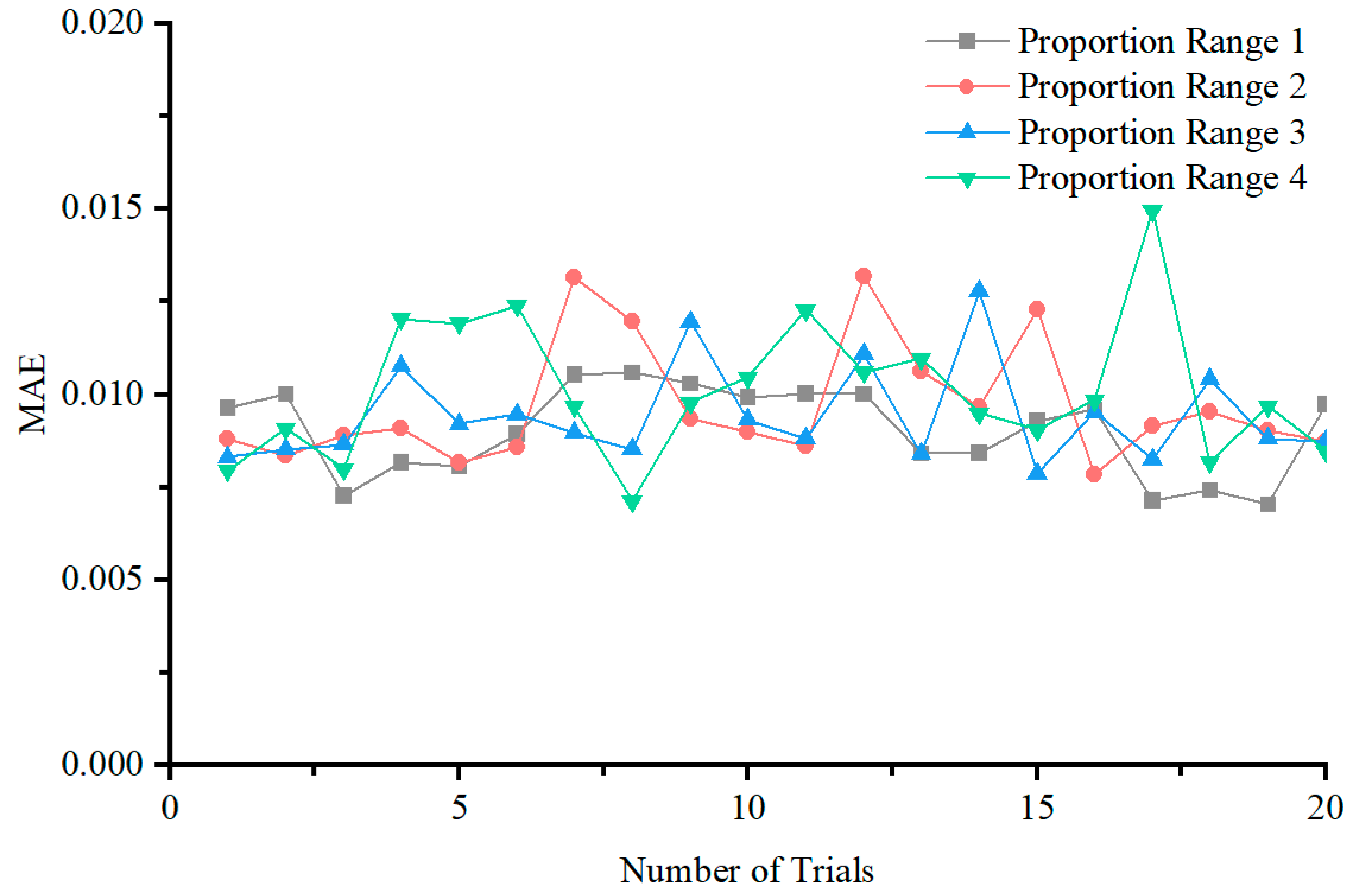
4.3.1. Elite Proportion

In DHEPSO, the elite proportion governs the ratio of high-performing particles that participate in guiding the search direction within the population. To enhance the algorithm’s adaptability across different optimization phases, an adaptive elite proportion adjustment mechanism is introduced in this study. To evaluate the performance of this mechanism under varying parameter configurations, multiple combinations of maximum and minimum elite proportion values were tested (as listed in Table 3), with 20 independent trials conducted for each configuration. The mean absolute error (MAE) between the simulated data and the fitted ellipsoid surfaces served as the evaluation metric for the comparative analysis.
Figure 4 displays the MAE line charts under various configurations. The results show that the varying elite proportion ranges have a minimal impact on the algorithm performance, as all the MAE curves exhibit comparable fluctuation ranges with no significant error increase. A comparison of the average MAE values from 20 independent trials yields 0.009025, 0.009701, 0.009419, and 0.0100096, where the current configuration achieves the lowest error among all candidate parameter sets. These findings confirm the robustness of the proposed adaptive elite proportion mechanism, which maintains stable performance across the parameter settings while balancing exploration and convergence, thereby ensuring consistent calibration accuracy.

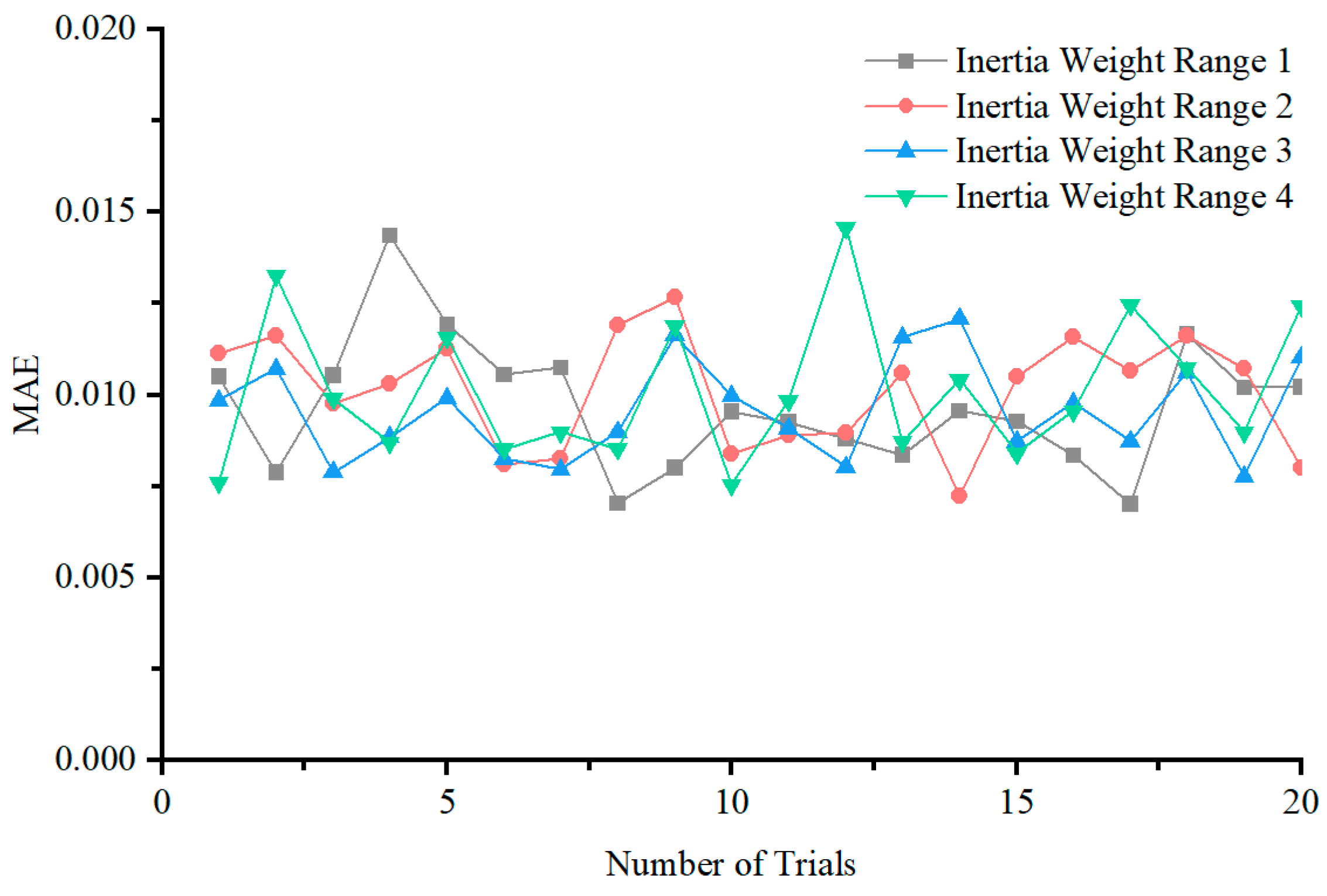
4.3.2. Inertia Weight

Inertia weight is a critical parameter governing particle swarm optimization’s global search capability and local convergence ability. DHEPSO incorporates an adaptive inertia weight adjustment mechanism designed to enhance exploration during the initial search phases and improve precision in the later convergence stages. To evaluate the impact of the inertia weight ranges on algorithmic performance, this study tested multiple combinations of maximum and minimum inertia weight values (as listed in Table 4), with 20 independent trials conducted for each configuration to ensure statistical reliability.
Figure 5 presents the MAE line charts across different configurations. The results demonstrate stable performance of the DHEPSO algorithm under various inertia weight combinations, with all MAE curves exhibiting small fluctuation ranges and no significant error escalation observed. The comparative analysis of the average MAE values from the 20 independent trials yields 0.009109, 0.010108, 0.009569, and 0.010132, where the currently implemented inertia weight range configuration achieves the lowest error level among all candidate solutions. These findings confirm the robustness of the proposed adaptive inertia weight mechanism in maintaining stable algorithmic performance within the tested parameter range.

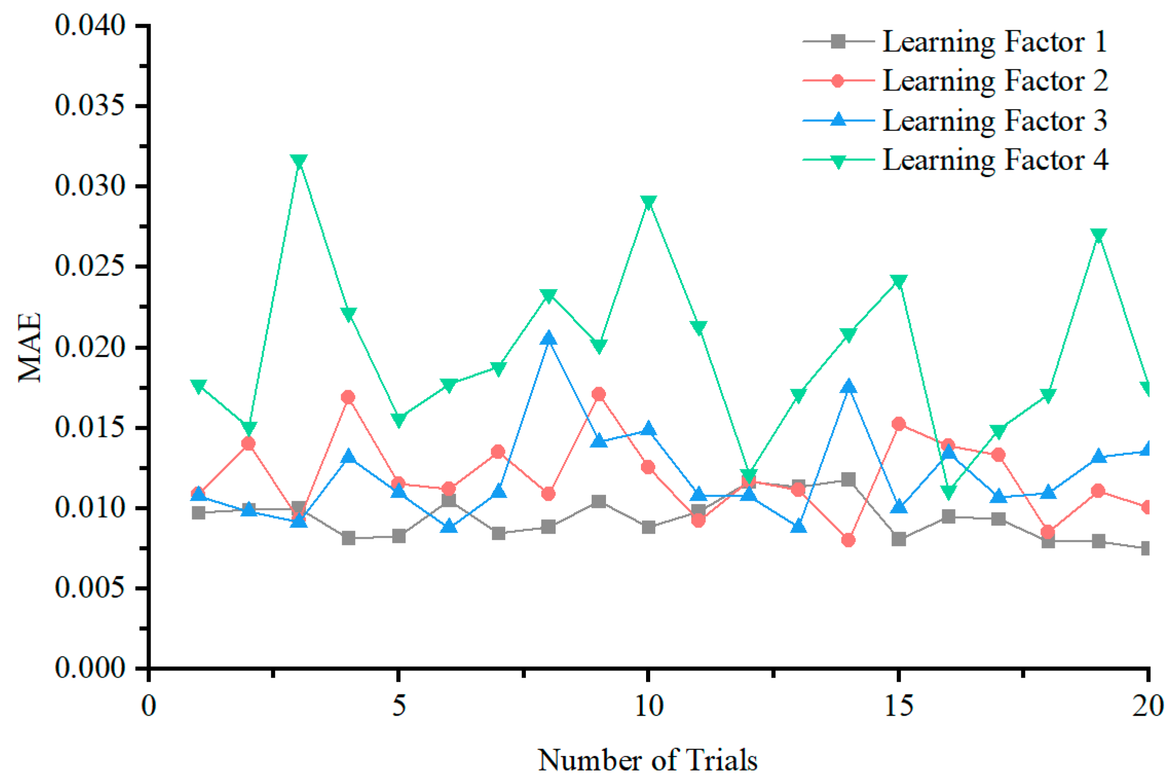
4.3.3. Learning Factor

Learning factors govern a particle’s learning capability from its personal historical best solution and the swarm’s global best solution. In this study, the learning factors are maintained at fixed values without implementing adaptive adjustment mechanisms. To systematically investigate their impact on algorithmic performance, this experiment tests multiple distinct learning factor combinations (as listed in Table 5), with 20 independent trials conducted for each configuration. The MAE serves as the evaluation metric for the comparative analysis.
Figure 6 presents the MAE line charts of 20 independent experimental trials. The results indicate that the learning factor settings significantly influence DHEPSO’s performance. Under certain configurations, the algorithm exhibits significant MAE fluctuations, with some parameter combinations failing to maintain results within acceptable error thresholds, demonstrating high sensitivity of algorithmic stability and precision to the learning factor selection. In contrast, the currently adopted learning factor configuration demonstrates superior stability and accuracy compared to the other candidate solutions.

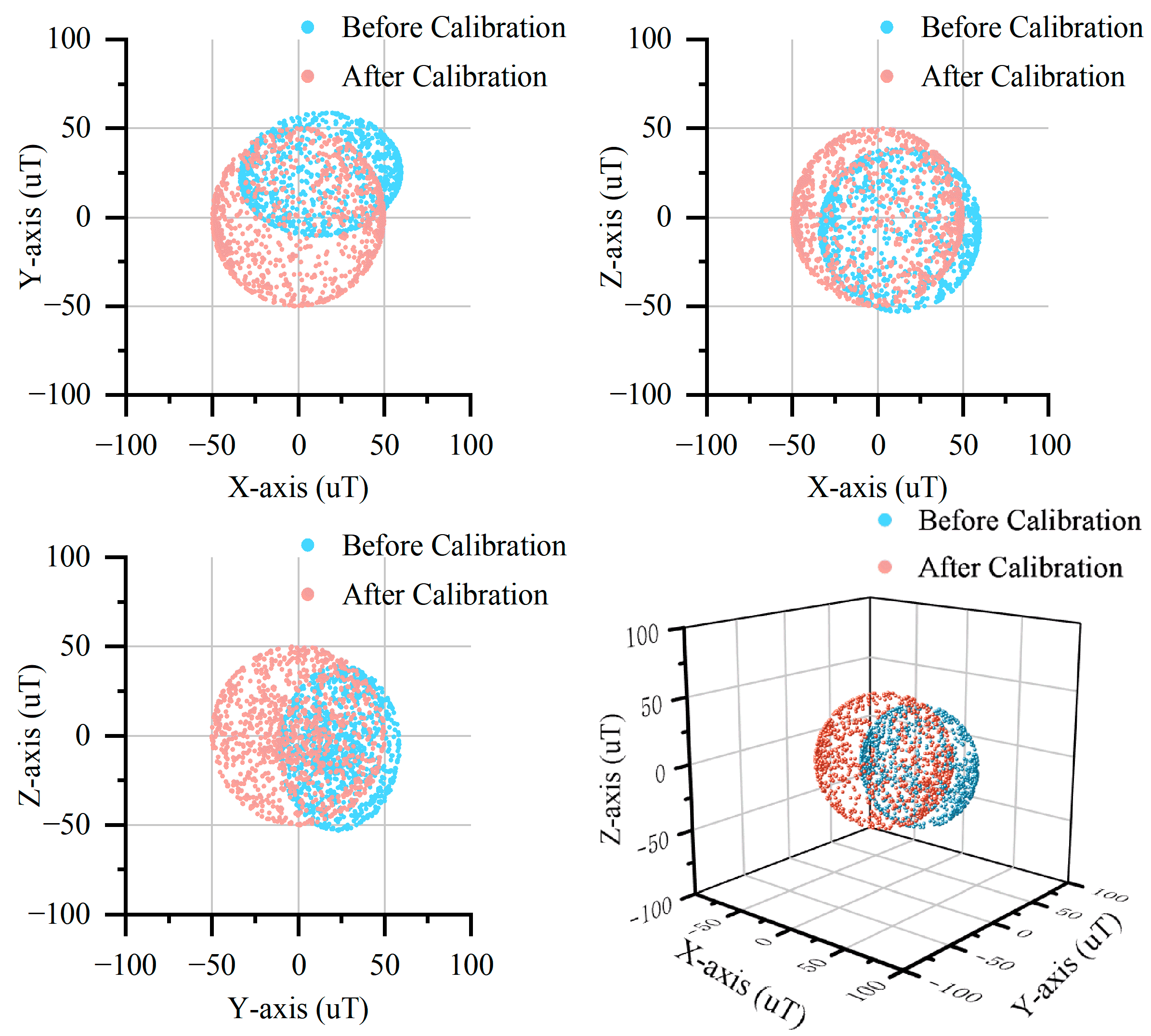
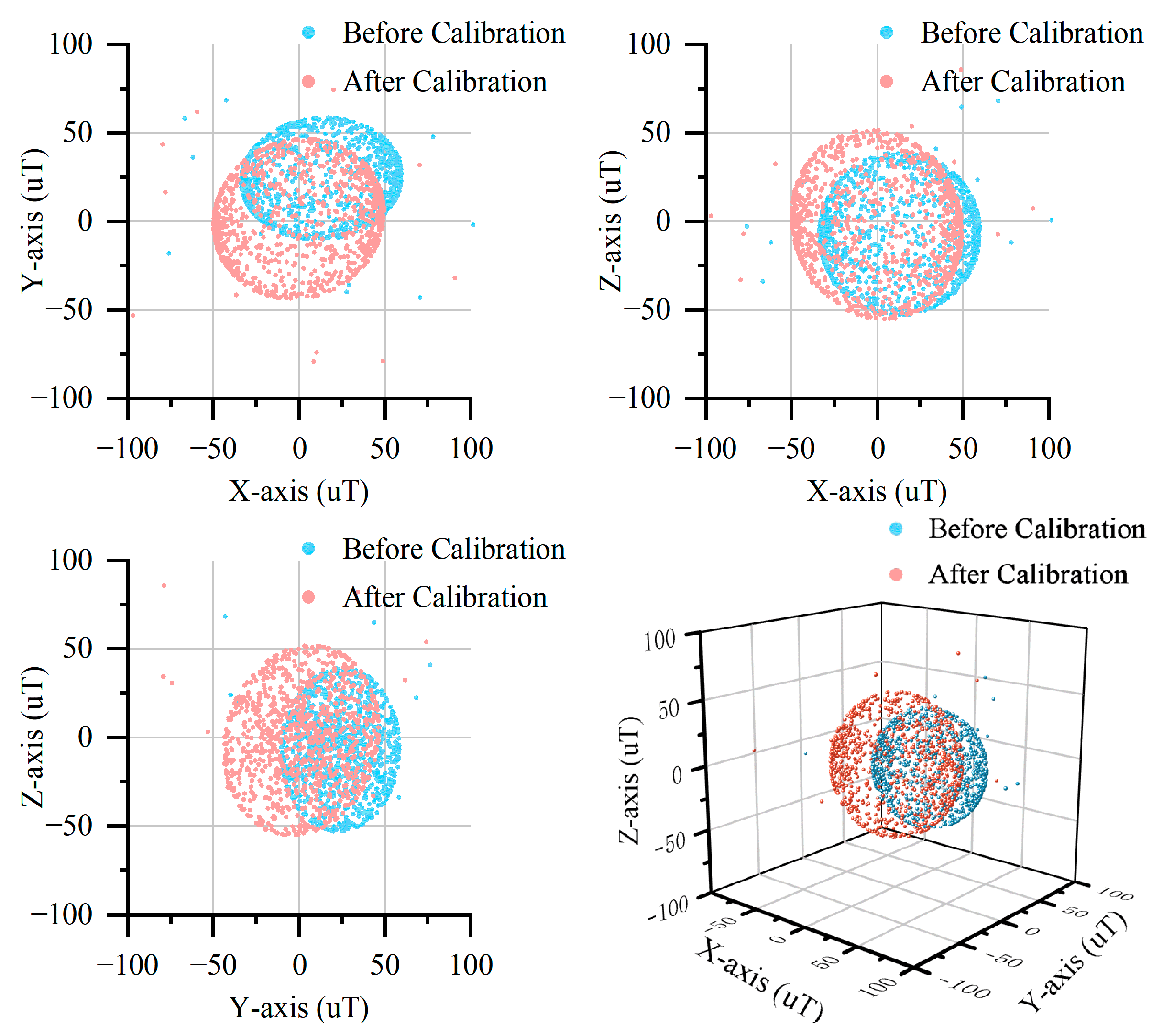
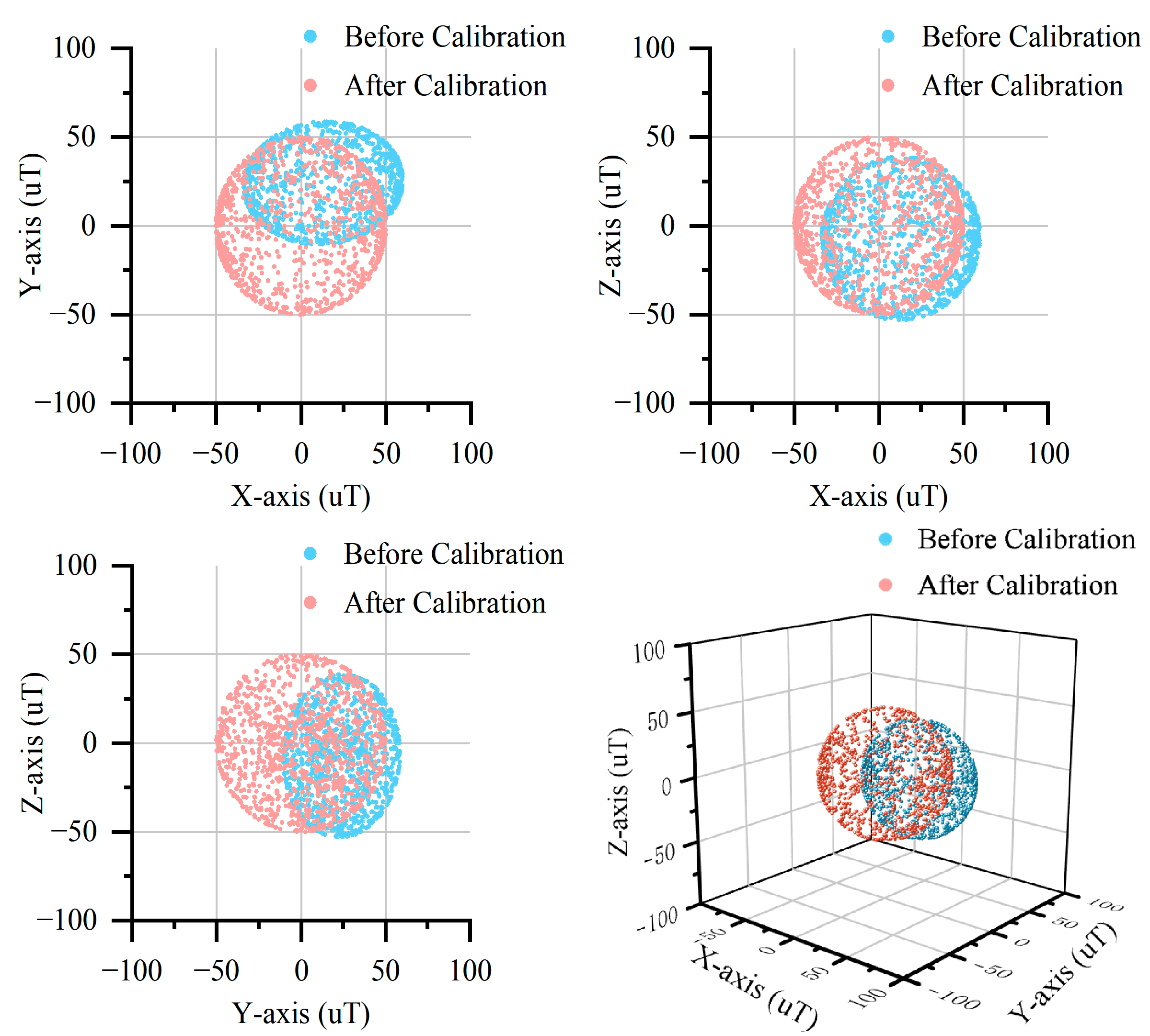
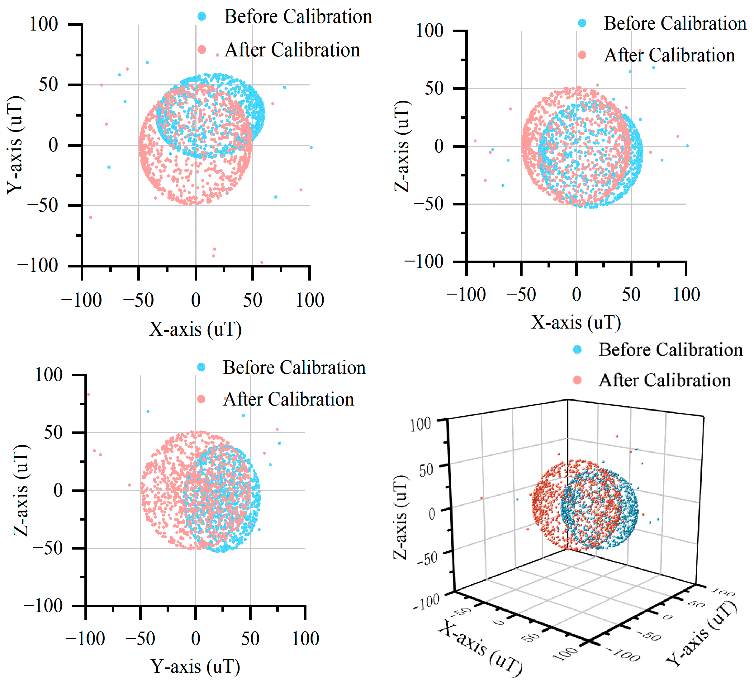
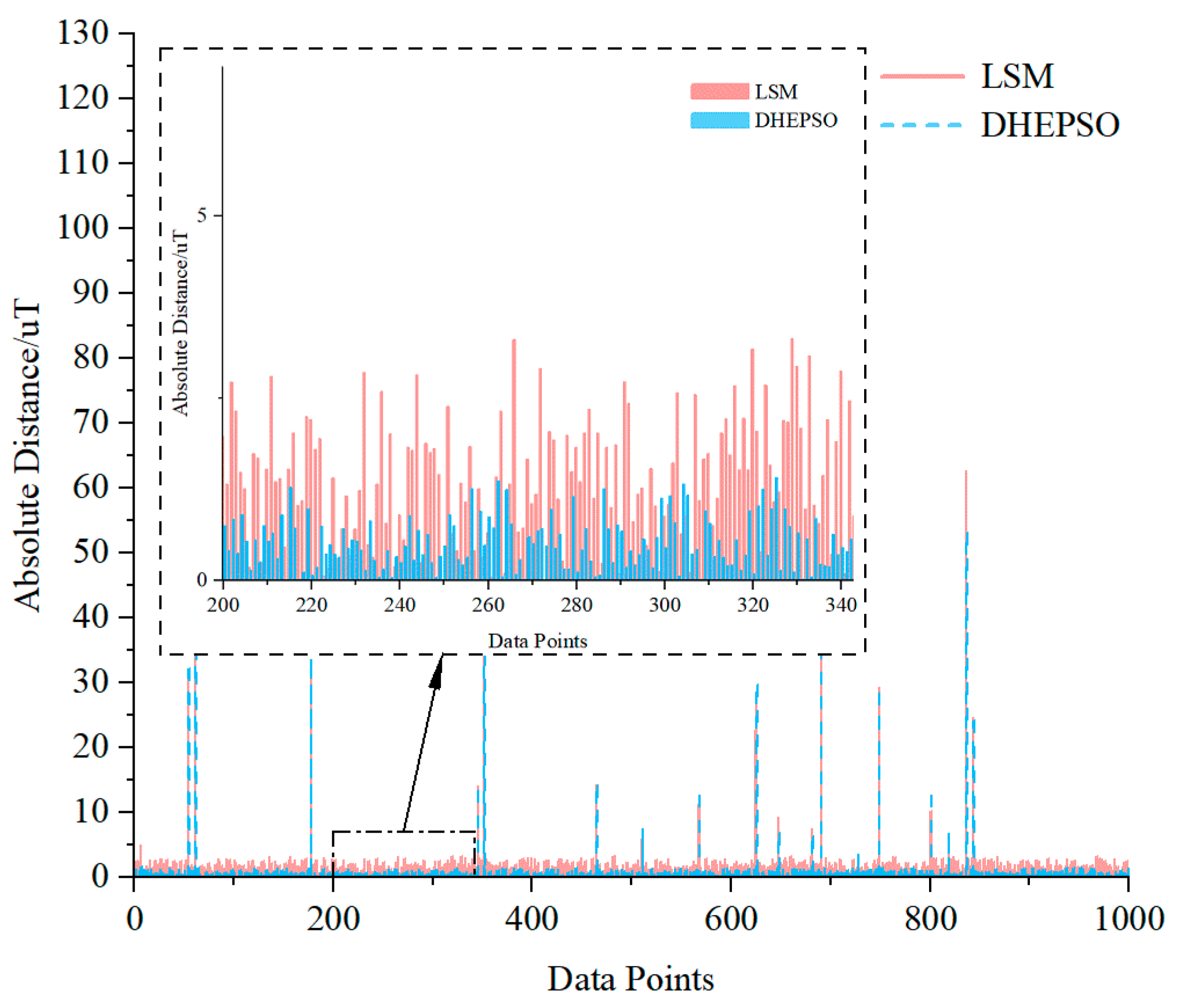
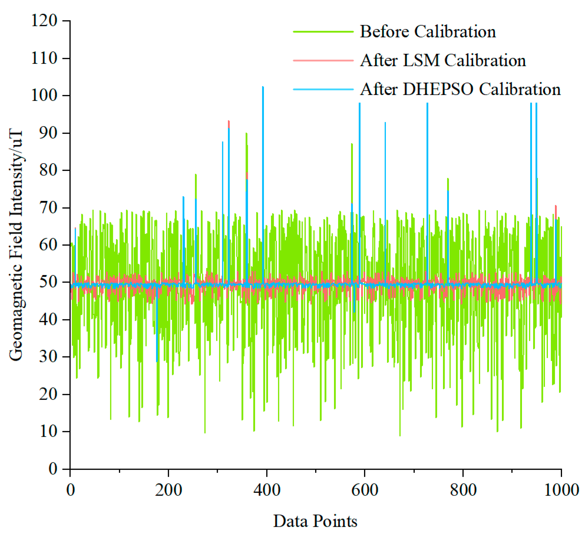
4.4. Comparative Analysis of DHEPSO and LSM

To validate the robustness of the DHEPSO algorithm in processing datasets containing outliers, a 2% outlier noise was introduced into the standard dataset to simulate extreme measurement errors. The comparative experiments with the LSM-based ellipsoid fitting algorithm were conducted to evaluate the anti-interference capability of the DHEPSO under outlier-contaminated conditions. The calibration results of both algorithms are presented in Figure 7, Figure 8, Figure 9, Figure 10, Figure 11 and Figure 12. Figure 7, Figure 8, Figure 9 and Figure 10, respectively, demonstrate the calibration performance of the two algorithms under outlier-free and outlier-contaminated scenarios; Figure 11 compares the absolute distances between the fitted ellipsoidal surfaces and the simulated data for both algorithms in the presence of outliers; Figure 12 illustrates the variations in total geomagnetic field intensity before and after calibration by the two algorithms under outlier interference.
As shown in Figure 7, Figure 8, Figure 9 and Figure 10, both the DHEPSO and LSM algorithms demonstrate comparable calibration performance on the outlier-free standard dataset, effectively achieving ellipsoid model fitting and error data correction. However, when processing noise-contaminated datasets containing outliers, the fitting results of the LSM algorithm are significantly disrupted, with calibrated results deviating from the ideal spherical distribution and exhibiting notable biases and instability. In contrast, the DHEPSO algorithm robustly suppresses outlier interference during optimization, maintaining high precision and stability in fitting outcomes.
As demonstrated in Figure 11, the superiority of DHEPSO in ellipsoid fitting is further validated. The comparative analysis based on 1000 simulated datasets reveals that the ellipsoidal surface constructed by DHEPSO exhibits tighter spatial alignment with data points than that of LSM. Specifically, when excluding outlier data, DHEPSO reduces the sum of absolute distances between the simulated data and the ellipsoid surface from 1423.86 µT (LSM) to 525.45 µT—a 63.10% improvement. This result confirms the enhanced parameter estimation accuracy and model fitting capability of the DHEPSO algorithm during ellipsoid fitting.
Figure 12 illustrates the variations in total magnetic field intensity before and after calibration. Prior to the calibration, the total magnetic field intensity exhibited significant fluctuations due to error interference, with a standard deviation of 14.20 µT. After calibration via the LSM-based ellipsoid fitting algorithm, the standard deviation decreased to 2.05 µT; however, residual fluctuations and deviations from the ideal value persisted. In contrast, the DHEPSO-based ellipsoid fitting algorithm demonstrated markedly improved calibration performance: the post-calibration intensity curve closely approached the ideal value, achieving a further reduced standard deviation of 0.82 µT—a 60% reduction compared to LSM-based calibration. These results unequivocally validate the superior parameter estimation accuracy of the DHEPSO algorithm.
The experimental results above demonstrate that the DHEPSO algorithm exhibits stronger anti-interference capability and robustness when processing outlier-contaminated data. Compared to the traditional LSM algorithm, DHEPSO effectively suppresses outlier interference, maintains high fitting accuracy and stability, and delivers optimized results closer to the theoretical ground truth, thereby providing a high-precision solution for practical applications.

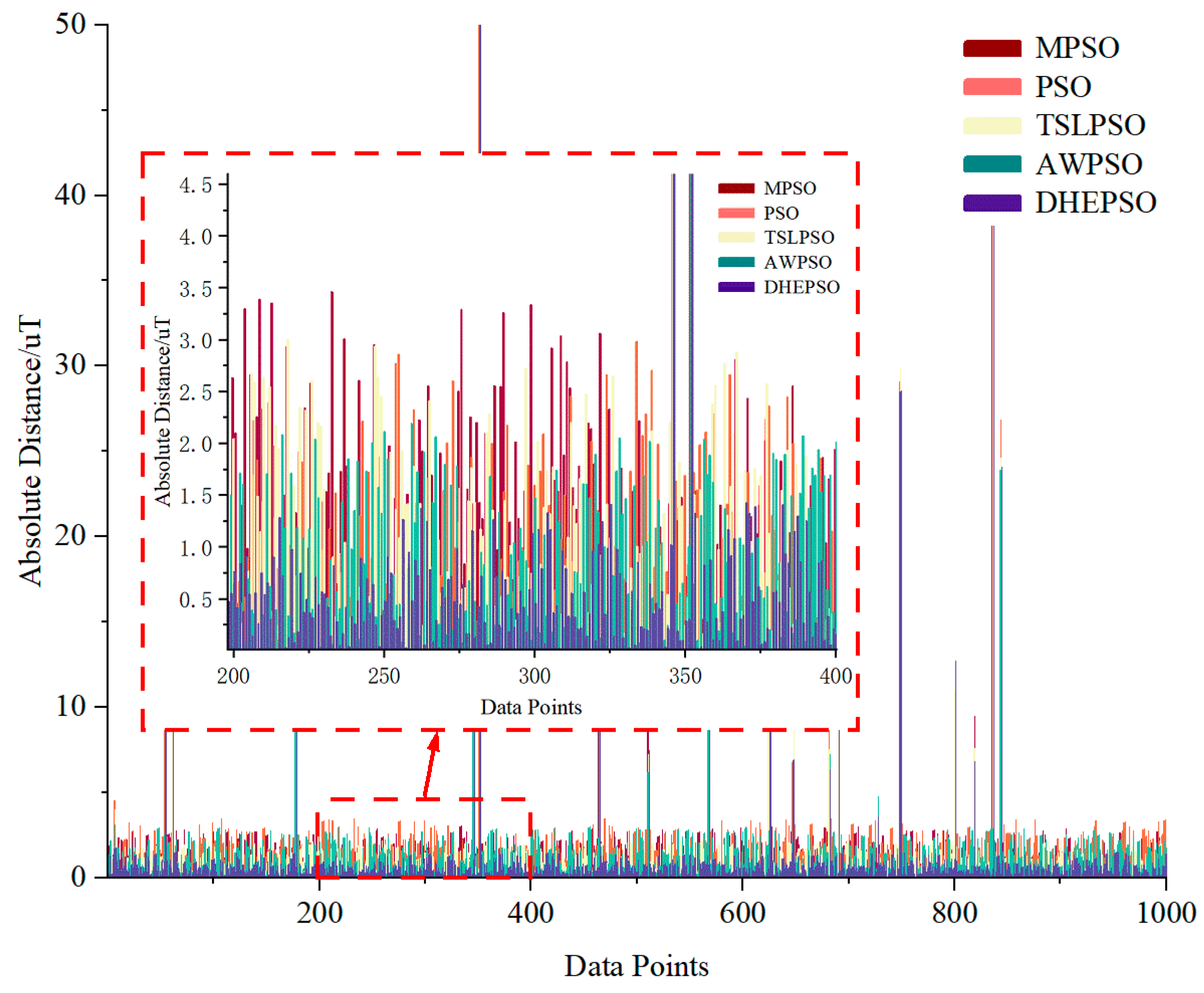
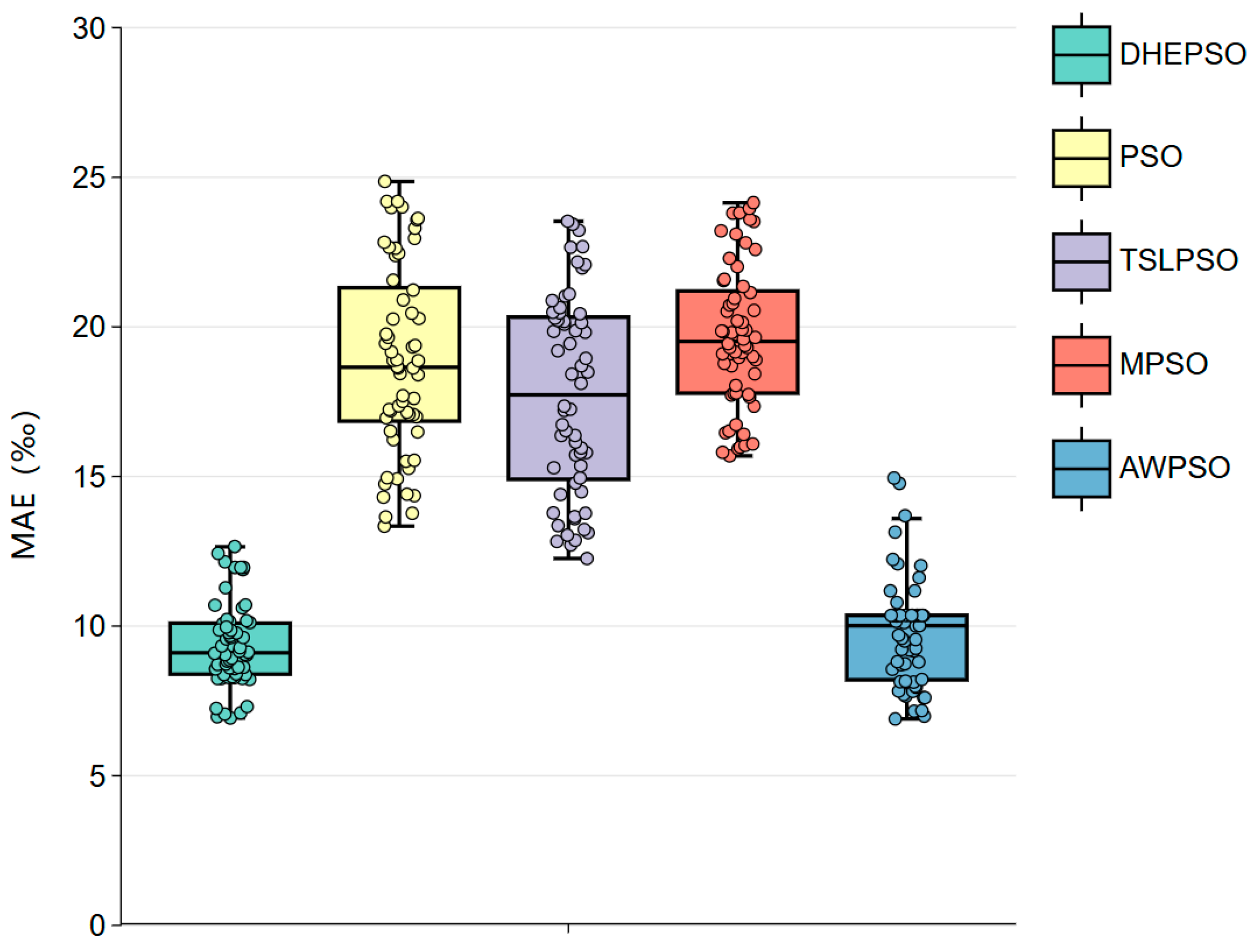
4.5. Comparative Analysis of PSO Variants

To further validate the convergence speed and precision of the proposed DHEPSO algorithm, a comparative analysis was conducted against the traditional PSO, TSLPSO, MPSO, and AWPSO. The parameter configurations for each compared algorithm are listed in Table 6.
The optimal convergence results were selected through multiple independent experiments, with the fitness convergence curves of all algorithms compared in Figure 13. Figure 13 reveals the fitness convergence characteristics during optimization. The DHEPSO algorithm exhibits a sharp decline in fitness values during the initial iterations, achieving convergence with fewer iterations compared to the traditional PSO, TSLPSO, MPSO, and AWPSO, thereby validating its efficient global search capability.
Figure 14 demonstrates the performance advantages of the DHEPSO algorithm over other PSO variants. When excluding outlier data, using the sum of absolute distances between the simulated data and the ellipsoid surface as the evaluation metric, DHEPSO (525.45 µT) achieves a 48.52% reduction compared to the traditional PSO (1020.63 µT). Its superiority remains pronounced against improved algorithms: a 47.74% reduction versus TSLPSO (1005.42 µT), 56.71% versus MPSO (1213.77 µT), and 33.09% versus AWPSO (785.27 µT). These results validate the superiority of the DHEPSO algorithm in parameter optimization mechanisms, effectively enhancing ellipsoid fitting precision.
To further evaluate the stability of the DHEPSO algorithm, this study conducted 60 independent repeated experiments for each algorithm, with performance comparisons based on the mean absolute error (MAE) between the simulated data and the fitted ellipsoid surface. The boxplot of error statistical results is presented in Figure 15. In the figure, the colored circles represent the MAE values obtained in each individual experiment. As evident from the figure, the DHEPSO algorithm exhibits superior median error and narrower interquartile range (IQR) compared to the other algorithms, demonstrating higher consistency and reliability. These findings validate its robustness advantages in high-interference environments.

5. Conclusions

This study addresses the calibration challenges of the triaxial magnetometers by integrating dynamic hierarchical mechanisms, elite guidance strategies, and adaptive inertia weight adjustment into the conventional PSO, proposing a DHEPSO-based ellipsoid fitting algorithm. Comparative analyses against the LSM, traditional PSO, TSLPSO, MPSO, and AWPSO yield the following conclusions:
  • Enhanced anti-interference capability: compared to the LSM-based ellipsoid fitting algorithm, the DHEPSO-based algorithm demonstrates superior resistance to outlier interference, higher fitting precision, and robust stability when processing outlier-contaminated data, effectively mitigating the impact of outliers on calibration processes.
  • Accelerated convergence performance: the DHEPSO algorithm achieves faster convergence than the traditional PSO, TSLPSO, MPSO, and AWPSO, efficiently locating global optima in ellipsoid fitting tasks, thereby exhibiting significant advantages in parameter optimization mechanisms.
  • Improved consistency and reliability: multiple independent experiments confirm that the DHEPSO-based algorithm outperforms comparative methods in median error and IQR, demonstrating enhanced reliability and consistency.
In summary, the proposed DHEPSO-based ellipsoid fitting algorithm exhibits superior comprehensive performance in high-interference environments. This methodology not only provides a novel solution for triaxial magnetometer calibration but also offers theoretical references for calibration problems of other sensors, demonstrating significant theoretical and practical significance for both academic research and engineering applications.

Author Contributions

Conceptualization, J.G. and Z.C.; methodology, J.G.; software, Z.C.; validation, J.G., Z.C. and G.J.; formal analysis, J.G.; investigation, Z.C.; resources, G.J.; data curation, Z.C.; writing—original draft preparation, J.G. and Z.C.; writing—review and editing, J.G. and G.J.; supervision, J.G. and G.J.; project administration, Z.C.; funding acquisition, J.G. All authors have read and agreed to the published version of the manuscript.

Funding

This research was funded by the National Natural Science Foundation of China under Grant No. 62203191, the Natural Science Foundation of the Jiangsu Higher Education Institutions of China under Grant No. 22KJB590001, National Key Laboratory of Defense Science and Technology under Grant No. 2022JCJQL06105, Basic Strengthening Program under Grant No. 2023JCJQJJ0357.

Data Availability Statement

The original contributions presented in this study are included in the article. Further inquiries can be directed to the corresponding author.

Conflicts of Interest

Author Guilin Jiang was employed by the company Huaihai Industries Group Co., Ltd. The remaining authors declare that the research was conducted in the absence of any commercial or financial relationships that could be construed as a potential conflict of interest.

References

  1. Sadaf, M.; Iqbal, Z.; Javed, A.R.; Saba, I.; Krichen, M.; Majeed, S.; Raza, A. Connected and automated vehicles: Infrastructure, applications, security, critical challenges, and future aspects. Technologies 2023, 11, 117. [Google Scholar] [CrossRef]
  2. Liu, W.; Hua, M.; Deng, Z.; Meng, Z.; Huang, Y.; Hu, C.; Song, S.; Gao, L.; Liu, C.; Shuai, B.; et al. A systematic survey of control techniques and applications in connected and automated vehicles. IEEE Internet Things J. 2023, 10, 21892–21916. [Google Scholar] [CrossRef]
  3. Long, D.; Zhang, X.; Wei, X.; Luo, Z.; Cao, J. A Fast Calibration and Compensation Method for Magnetometers in Strap-Down Spinning Projectiles. Sensors 2018, 18, 4157. [Google Scholar] [CrossRef]
  4. Fang, X.; Wang, L. Study and Numerical Simulation of the Standardizing Method of Geomagnetic Sensor. J. Proj. Rocket. Missiles Guid. 2018, 38, 73–76. [Google Scholar]
  5. Zhi, Z.W.; Gao, K.; Chu, Z.W.; Lin, W.; Lin, X.H. A Calibration Method of Magnetic Compass Based on Non-iterative Ellipsoid Fitting. Instrum. Technol. 2020, 3–6. [Google Scholar] [CrossRef]
  6. Peng, J.B.; Zhang, X.L.; Zhang, W.; Yao, X.T. Calibration Method for Measurement Error Parameters of Three-Axis Magnetic Sensors. J. Gun Launch Control 2025, 1–7. [Google Scholar] [CrossRef]
  7. Zhimin, L.I.; Jizhou, L.A.; Pin, L.Y. Experimental design for rapid calibration of three-axis magnetic sensors based on ellipsoidal fitting. Exp. Technol. Manag. 2023, 40, 42–47. [Google Scholar]
  8. Gong, X.; Song, Z.; Xi, X. Error calibration of three axis magnetometer based on Global Artificial Fish Swarm Algorithm. In Proceedings of the 2013 IEEE International Conference of IEEE Region 10 (TENCON 2013), Xi’an, China, 22–25 October 2013; pp. 1–4. [Google Scholar]
  9. Yang, L.; Li, C.; Zhang, S.; Xu, C.; Chen, H.; Xiao, S.; Tang, X.; Li, Y. Correction method of three-Axis magnetic sensor based on DA–LM. Metals 2022, 12, 428. [Google Scholar] [CrossRef]
  10. Li, X.; Yan, S.; Liu, J.; Sun, Y.; Yan, Y. Partition beetles antennae search algorithm for magnetic sensor calibration optimization. IEEE Sens. J. 2020, 21, 5967–5974. [Google Scholar] [CrossRef]
  11. Pang, X.L.; Lin, C.S. Calibration Coefficients Solving of Three-Axis Magnetic Sensor Based on Genetic Algorithm. J. Detect. Control 2017, 39, 42–45+51. [Google Scholar]
  12. Pang, H.; Zhang, Q.; Wang, W.; Wang, J.; Li, J.; Luo, S.; Wan, C.; Chen, D.; Pan, M.; Luo, F. Calibration of three-axis magnetometers with differential evolution algorithm. J. Magn. Magn. Mater. 2013, 346, 5–10. [Google Scholar] [CrossRef]
  13. Huang, H.; Wang, P.; Shen, H. Magnetometer error compensation algorithm based on immune adaptation particle swarm optimization algorithm. In Proceedings of the 2021 International Conference on Sensing, Measurement & Data Analytics in the era of Artificial Intelligence (ICSMD), Nanjing, China, 21–23 October 2021; pp. 1–5. [Google Scholar]
  14. Wu, Z.; Wu, Y.; Hu, X.; Wu, M. Calibration of three-axis magnetometer using stretching particle swarm optimization algorithm. IEEE Trans. Instrum. Meas. 2012, 62, 281–292. [Google Scholar] [CrossRef]
  15. Lei, X.; Zhang, X.; Hao, Y. An intelligent ellipsoid calibration method based on the grey wolf algorithm for magnetic compass. J. Bionic Eng. 2021, 18, 453–461. [Google Scholar] [CrossRef]
  16. Chafi, M.R.S.; Narm, H.G.; Kalat, A.A. Calibration of fluxgate sensor using least square method and particle swarm optimization algorithm. J. Magn. Magn. Mater. 2023, 570, 170364. [Google Scholar] [CrossRef]
  17. Nerrise, F.; Sosanya, A.S.; Neary, P. Physics-informed calibration of aeromagnetic compensation in magnetic navigation systems using liquid time-constant networks. arXiv 2024, arXiv:2401.09631. [Google Scholar]
  18. Tian, D.; Li, Y.; Jin, M.; Guo, Y.; Meng, F.; Liu, Q. Data-Driven Calibration of Tri-axial Magnetic Sensors. Meas. Sci. Technol. 2025, 36, 035117. [Google Scholar] [CrossRef]
  19. Cowart, J., III; Petrich, J. Three-dimensional magnetometer calibration using higher order models embedded into neural networks. Robot. Auton. Syst. 2025, 186, 104903. [Google Scholar] [CrossRef]
  20. Zikmund, A.; Janosek, M.; Ulvr, M.; Kupec, J. Precise calibration method for triaxial magnetometers not requiring earth’s field compensation. IEEE Trans. Instrum. Meas. 2015, 64, 1242–1247. [Google Scholar] [CrossRef]
  21. Tabatabaei, S.A.H.; Gluhak, A.; Tafazolli, R. A fast calibration method for triaxial magnetometers. IEEE Trans. Instrum. Meas. 2013, 62, 2929–2937. [Google Scholar] [CrossRef]
  22. Ye, L.; Yu, Z.; Zhang, Y.; Chi, C.; Cheng, P.; Chen, J. An aeromagnetic compensation strategy for large uavs. Sensors 2024, 24, 3775. [Google Scholar] [CrossRef]
  23. Yu, H.; Guo, Y.; Ye, L.; Han, T.; Su, S.W. Experimental Design for the Inclination based Linear Magnetometers Calibration Method. IEEE Trans. Instrum. Meas. 2024, 73, 1005609. [Google Scholar] [CrossRef]
  24. Klingbeil, L.; Eling, C.; Zimmermann, F.; Kuhlmann, H. Magnetic field sensor calibration for attitude determination. J. Appl. Geod. 2014, 8, 97–108. [Google Scholar] [CrossRef]
  25. Jiang, W.; Tan, X. Improved ellipsoid fitting aided geomagnetic sensor calibration algorithm. Meas. Sci. Technol. 2024, 35, 076302. [Google Scholar] [CrossRef]
  26. Hu, F.; Wu, Y.; Yu, Y.; Nie, J.; Li, W.; Gao, Q. An improved method for the magnetometer calibration based on ellipsoid fitting. In Proceedings of the 2019 12th International Congress on Image and Signal Processing, Biomedical Engineering and Informatics (CISP-BMEI), Suzhou, China, 19–21 October 2019; pp. 1–5. [Google Scholar]
  27. An, L.L.; Wang, L.M.; Zhong, Y. Ellipsoid fitting compensation method for three-axis magnetometer on projectile. Transducer Microsyst. Technol. 2020, 39, 4–6+13. [Google Scholar]
  28. Zhou, Q.; Yao, M.L.; Shen, X.W. Research on Field Calibration Method for MEMS Accelerometer Based on Support Ellipsoid Fitting. Acta Armamentarii 2020, 41, 68–74. [Google Scholar]
  29. Ramírez-Ochoa, D.D.; Pérez-Domínguez, L.A.; Martínez-Gómez, E.A.; Luviano-Cruz, D. PSO, a swarm intelligence-based evolutionary algorithm as a decision-making strategy: A review. Symmetry 2022, 14, 455. [Google Scholar] [CrossRef]
  30. Tharwat, A.; Schenck, W. A conceptual and practical comparison of PSO-style optimization algorithms. Expert Syst. Appl. 2021, 167, 114430. [Google Scholar] [CrossRef]
  31. Jain, M.; Saihjpal, V.; Singh, N.; Singh, S.B. An overview of variants and advancements of PSO algorithm. Appl. Sci. 2022, 12, 8392. [Google Scholar] [CrossRef]
  32. Yang, C.; Gao, W.; Liu, N.; Song, C. Low-discrepancy sequence initialized particle swarm optimization algorithm with high-order nonlinear time-varying inertia weight. Appl. Soft Comput. 2015, 29, 386–394. [Google Scholar] [CrossRef]
  33. Liu, Y.; Xiao, W.; Wu, J.; Zhao, K. Calibration method of magnetic and inertial sensors based on Newton iteration and ellipsoid fitting. Chin. J. Sci. Instrum. 2020, 41, 142–149. [Google Scholar]
  34. Zhao, H.; Su, Z.; Liu, F.; Li, C.; Li, Q. Magnetometer-based phase shifting ratio method for high spinning projectile’s attitude measurement. IEEE Access 2019, 7, 22509–22522. [Google Scholar] [CrossRef]
  35. Marini, F.; Walczak, B. Particle swarm optimization (PSO). A tutorial. Chemom. Intell. Lab. Syst. 2015, 149, 153–165. [Google Scholar] [CrossRef]
  36. Xu, G.; Cui, Q.; Shi, X.; Ge, H.; Zhan, Z.H.; Lee, H.P.; Liang, Y.; Tai, R.; Wu, C. Particle swarm optimization based on dimensional learning strategy. Swarm Evol. Comput. 2019, 45, 33–51. [Google Scholar] [CrossRef]
  37. Liu, H.; Zhang, X.W.; Tu, L.P. A modified particle swarm optimization using adaptive strategy. Expert Syst. Appl. 2020, 152, 113353. [Google Scholar] [CrossRef]
  38. Liu, W.; Wang, Z.; Yuan, Y.; Zeng, N.; Hone, K.; Liu, X. A novel sigmoid-function-based adaptive weighted particle swarm optimizer. IEEE Trans. Cybern. 2019, 51, 1085–1093. [Google Scholar] [CrossRef]
Figure 1. Flowchart of the ellipsoid fitting algorithm.
Electronics 14 01778 g001
Figure 2. Workflow of the DHEPSO algorithm.
Electronics 14 01778 g002
Figure 3. Flowchart of the DHEPSO-based ellipsoid fitting algorithm.
Electronics 14 01778 g003
Figure 4. MAE Line Charts for Different Elite Proportion Ranges.
Electronics 14 01778 g004
Figure 5. MAE Line Charts for Different Inertia Weight Ranges.
Electronics 14 01778 g005
Figure 6. MAE Line Charts for Different Learning Factor.
Electronics 14 01778 g006
Figure 7. Results of LSM-based Ellipsoid Fitting Calibration (Outlier-Free).
Electronics 14 01778 g007
Figure 8. Results of LSM-based Ellipsoid Fitting Calibration (Outlier-Contaminated).
Electronics 14 01778 g008
Figure 9. Results of DHEPSO-based Ellipsoid Fitting Calibration (Outlier-Free).
Electronics 14 01778 g009
Figure 10. Results of DHEPSO-based Ellipsoid Fitting Calibration (Outlier-Contaminated).
Electronics 14 01778 g010
Figure 11. Absolute Distance from Simulated Data to Ellipsoid Surface: LSM vs. DHEPSO.
Electronics 14 01778 g011
Figure 12. Total Geomagnetic Field Intensity Before and After Calibration.
Electronics 14 01778 g012
Figure 13. Fitness Convergence Curves of Different PSO Algorithms.
Electronics 14 01778 g013
Figure 14. Absolute Distances from Simulated Data to Ellipsoid Surface: PSO Variants.
Electronics 14 01778 g014
Figure 15. Boxplots of Mean Absolute Errors over 60 Independent Runs: PSO Variants.
Electronics 14 01778 g015
Table 1. Initialization Parameters of DHEPSO.
Parameter NameSymbolValue/Range
Population Size N P 100
Parameter Dimension d i m 10
Maximum Iterations T 500
Inertia Weight ω [0.5, 0.7]
Minimum Elite Proportion r min 0.05
Maximum Elite Proportion r max 0.15
Elite Layer Individual Learning Factor c 1 e 2.0
Elite Layer Swarm Learning Factor c 2 e 1.5
Ordinary Layer Individual Learning Factor c 1 n 1.5
Ordinary Layer Swarm Learning Factor c 2 n 2.0
Elite Guidance Term Learning Factor c 3 n 0.1
Table 2. Parameters of the Triaxial Magnetometer Numerical Simulation Model.
ParameterValue
Geomagnetic Field Intensity/µT50
Magnetic Declination/°−5.8
Magnetic Inclination/°49.0
Sensitivity Error d i a g 1.113 0.904 1.107
Non-Orthogonality Error 1 0 0.0028 0.0026 1 0.0035 0 0 1
Zero-Offset Error/µT 2.0 3.0 4.0 T
Soft-Iron Interference 0.84 0.053 0.026 0.082 0.72 0.012 0.016 0.034 0.83
Hard-Iron Interference/µT 10.0 30.0 10.0 T
Table 3. Configuration Table of Elite Proportion.
Parameter SetValue
Proportion Range 1(0.05, 0.15)
Proportion Range 2(0.04, 0.2)
Proportion Range 3(0.03, 0.3)
Proportion Range 4(0.02, 0.4)
Table 4. Configuration Table of Inertia Weight.
Parameter SetValue
Inertia Weight Range 1(0.5, 0.7)
Inertia Weight Range 2(0.4, 0.8)
Inertia Weight Range 3(0.3, 0.9)
Inertia Weight Range 4(0.2, 1.0)
Table 5. Configuration Table of Learning Factor.
Parameter SetValue
Learning Factor 1 c 1 e 2.0
c 2 e 1.5
c 1 n 1.5
c 2 n 2.0
Learning Factor 2 c 1 e 2.5
c 2 e 1.5
c 1 n 1.5
c 2 n 2.5
Learning Factor 3 c 1 e 2.8
c 2 e 1.2
c 1 n 1.2
c 2 n 2.8
Learning Factor 4 c 1 e 2.5
c 2 e 2.0
c 1 n 2.0
c 2 n 2.5
Table 6. Parameters of PSO Variants.
AlgorithmParameters
PSO c 1 = 1.5 ,   c 2 = 2.5 ,   w : 0.7 0.5
TSLPSO c 1 = c 2 = 1.5 ,   c 3 : 0.5 2.5 ,   w : 0.9 0.4
MPSO c 1 = c 2 = 2 ,   w : 0.9 0.4
AWPSO w : 0.9 0.5 ,   a = 0.000035 m ,   b = 0.5 ,   c = 0 ,   d = 1.5
Disclaimer/Publisher’s Note: The statements, opinions and data contained in all publications are solely those of the individual author(s) and contributor(s) and not of MDPI and/or the editor(s). MDPI and/or the editor(s) disclaim responsibility for any injury to people or property resulting from any ideas, methods, instructions or products referred to in the content.

