Distributed Adaptive Formation Control for Second-Order Multi-Agent Systems Without Collisions

Abstract

This paper presents an adaptive strategy to solve the formation control problem for a set of second-order agents with parametric uncertainty and nonlinearity. The strategy regards a group of agents where the nonlinearities and uncertainties are represented by a linearly parametrized term, which allows us to consider non-identical agents. In order to ensure the collision-free motion of agents, we propose the use of a repulsive vector field component that is applied only when a pair of agents becomes nearer than a predefined minimum bound. Numerical simulations were carried out to show the effectiveness of the proposed scheme. First, a simplified example was used to verify the key features of the control law, followed by a general case to illustrate the performance of the algorithm in a more complex scenario.

1. Introduction

The study of multi-agent systems (MASs) has significantly increased over the last few decades, driven by technological advancements that have supported the application of these schemes in a wide variety of fields such as agriculture, patrolling, search and rescue, etc. [1,2,3,4,5]. In this kind of system, a group of agents can perform tasks that—for a single robot—could be very difficult or even impossible. Among the main advantages of MASs are modularity, scalability, and decentralization of tasks among the different members of the group. In this research area, several issues have been studied, e.g., formation control, synchronization, path following, and containment control, among others [6,7,8,9].

In the formation control problem, agents have to reach a specific relative position or form a desired geometric pattern. This spatial distribution could be specified by global positions, inter-agent distances, or relative displacements, known as position-based, displacement-based, and distance-based, respectively. In each mentioned case, depending on the type of robot, agents need different sensor and communication capabilities to achieve the desired goal [10]. In a position-based scheme, communication between agents is not needed, and agents are supposed to have access to their global positions, allowing them to reach their desired location without any interaction with other members of the group. On the other extreme, distance-based strategies only specify desired distances among agents, which, depending on the initial conditions and the robot’s sensing accuracy, can lead to a translated or rotated formation. Displacement-based strategies, serving as the midpoint, enable enhanced performance by utilizing various decentralization levels to optimize the resources dictated by the chosen robot model. The approaches mentioned have been applied to various types of robots, including those modeled by single or double integrators, unicycle robots, and high-order linear systems. These applications also consider a number of additional constraints such as input saturation, failing actuators, time-delay communication, parametric uncertainty, etc.

In order to enhance the applicability of the proposed algorithm, considerable efforts have been made to incorporate more general models. These models better represent the realistic behaviors of physical systems and account for constraints imposed by the structure or equipment of the selected robots, such as parametric uncertainty and non-linearity [11]. To this end, second-order models can be a middle point between the complexity of a realistic representation of a robotic system and the advantage of being abstract enough to capture some key features. The optimal time-invariant formation tracking problem was studied in [12] for second-order agents. There, it was assumed that all agents have identical dynamics, and each one has access to their absolute position and velocity. In [13], uncertain second-order systems were studied. The authors assumed that the parameters of each robot could be different but known. Strategies were proposed to achieve formation tracking of the desired formation under switching directed topologies. In [14], the authors proposed a distributed adaptive control strategy for distance-based formation and flocking control. Nonidentical second-order agents were considered with unknown constant parameters, which were linearly parametrizable. Global convergence to the desired formation and the leader’s velocity was achieved. In [15], strategies were developed for agents to achieve formation tracking control under a leader-follower scheme, accommodating both constant and time-varying leader velocities. Estimators to compensate for the uncertainties were designed, and PI-like controllers using the stress matrix were designed. The backstepping technique was applied in [16] to estimate the uncertain parameters of the neighboring agents as well as the desired trajectory parameters when the agents did not have access to global information. Recently, in [17], an adaptive backstepping approach in combination with neural networks was proposed to solve the optimal formation control problem in finite time. In this work, more general uncertain dynamics are assumed, where the nonlinear term is locally Lipschitz. Recently, data-driven control algorithms were applied to formation control research given their ability to design control laws based on local measurements to overcome mismatches in models and/or parameters. In [18], an optimal controller was proposed for a group of quadrotors with unknown dynamics, while in [19], this idea was extended to a heterogeneous group of agents. Another interesting work with this approach can be found in [20], where a finite-time solution to the formation control problem was proposed by using the motion of the leader in a group of second-order agents. Learning techniques have also been applied to this area; for example, in [21], inverse reinforcement learning was used to manage disturbances in a heterogeneous MAS. An event-trigger approach has also been exploited in the formation control problem, for example, in [22], circle formation was studied for a group of second-order agents with ring-like communication topology. Results were conservative because of the use of linear matrix inequalities (LMIs) and the assumption of knowing exactly the dynamics of agents. In [23], the event-trigger protocol is combined with a persistent excitation condition to design a dynamic scheme for second-order nonholonomic agents. Additionally, techniques, such as adaptive fuzzy control, have been applied to manage nonlinearities of second-order agents [24,25,26,27].

On the other hand, one of the most important issues in MASs—when they are meant to be deployed in real applications—involves collision avoidance between agents or against obstacles in dynamic environments. This issue has been studied using a number of approaches. In [28], avoidance functions with finite cutoff were designed and avoidance control was given by the gradient of potential functions. Distance and velocity information were taken into account in [29] to clearly identify the situations that could lead to collisions, to reduce energy consumption and minimize the impact of the avoidance potential field on formation maintenance. A learning-based strategy to solve the formation control problem with collision avoidance was proposed in [30] by combining neural networks and the artificial potential field technique. In [31], a scheme based on neural networks and improved potential functions was proposed for second-order uncertain systems with disturbances. Recently, in [32], a fuzzy logic controller was proposed to solve the formation control problem for a group of unmanned aerial vehicles, where collision-free motion was guaranteed by applying the artificial potential method. In [33], a solution based on a limited angular field-of-view is proposed by using a probabilistic approach. In the same way, geometrical approaches have been utilized to prevent collisions along with potential functions [34]. These approaches have been used in diverse applications such as aerial, underwater, or surface vessels [35,36,37].

In this paper, a solution to the formation control problem without collisions is proposed regarding a general uncertain model for second-order agents. The strategy regards a group of agents where the nonlinearities and uncertainties are represented by a linearly parametrized term, which allows us to consider non-identical agents. We assume that the communication among agents is such that there exists, at least, a directed spanning tree. Inspired by an algorithm previously developed for first-order systems, we propose an extension for second-order systems by using a backstepping-like technique. Moreover, uncertainty and nonlinearity in the form of a parametrizable structure are added to each agent. This uncertain term is compensated for by a local adaptive component in the control law.

To ensure the collision-free motion of agents, we propose the use of repulsive vector fields that are applied only when agents come closer than a predefined minimum distance. These vector fields are designed using an unstable focus structure in such a way that no undesired equilibria exist, that is, preventing agents from becoming stuck in undesired configurations. This additional component of the control law is position- and velocity-based and is activated in a smooth way by using a bounded switching function.

In order to distinguish between the effect of local uncertainty and the influence of other surrounding agents, the adaptation law is only applied when there is no risk of collision, that is, each agent estimates its own parameters only when there are no other agents in its detection region. Otherwise, the agent retains the last estimated value of parameters, and a repulsive vector field is enabled to guarantee collision-free motion. When the conflict is solved, that is, when agents are far away from each other and there are no threatening agents, the adaptation law is restarted, taking the last saved parameter values.

To summarize, the main novelty of our work involves the use of adaptation laws in combination with smooth repulsive vector fields, giving priority to the avoidance control to ensure a collision-free motion, but compensating for parametric uncertainty locally to achieve the formation objective asymptotically.

The remainder of the paper is organized as follows. In Section 2, we review some important concepts in graph theory and recall some well-known lemmas. We formally state the problem in Section 3, and in Section 4, we present our main contribution. Numerical simulations were performed to show the performance of the proposed algorithms, whose results are presented in Section 5. Finally, some conclusions and outlines for the next stages of this research are listed in Section 6.

2. Preliminaries

In this section, we recall some important graph theory concepts as well as some lemmas that will be useful in the rest of the paper.

Communication among a group of agents is represented through a formation graph $G=\{V,E,C\}$, which consists of a set of vertices $V=\{R_1,\dots ,R_n\}$ representing the agents. The graph also includes a set of edges $E=\{\left(R_j{R}_i\right)\in V\times V,i\ne j\}$, where each edge indicates that agent $R_i$ receives information from agent $R_j$. Here, $R_j$ is called the parent node and $R_i$ is called the child node. Furthermore, there is a set $C=\{c_{ji}\in R^2|\left(R_j{R}_i\right)\in E,i\ne j\}$ that contains constant vectors that specify the desired relative position of agent $R_i$ regarding its neighbors.

A formation graph is undirected if, for any $\left(R_j{R}_i\right)\in E$, the reverse $\left(R_i{R}_j\right)\in E$ also holds, indicating bidirectional communication. In contrast, the graph is considered directed if $\left(R_i{R}_j\right)\in E$ does not imply $\left(R_i{R}_j\right)\in E$. When a formation graph is neither solely directed nor undirected, it is classified as mixed. There is a path connecting the vertices $R_j$ and $R_i$ if there is a succession of edges as follows: $\left(R_j{R}_{m_1}\right),\left(R_{m_1}{R}_{m_2}\right),\dots ,\left(R_{m_r}{R}_i\right)$, with $i\ne j$. A directed tree is defined as a directed graph in which each node, except one, called the root, has a single parent. The root lacks a parent and has a direct path to all other nodes. A directed tree incorporating all nodes of a directed graph G is termed a directed spanning tree.

For a given graph G, its Laplacian matrix is expressed as

$$\mathcal{L}\left(G\right)=\Delta -{\mathcal{A}}_d,$$

where the degree matrix $\Delta$ is specified by $\Delta =\mathrm{diag}\{g_1,\dots ,g_n\}$, with $g_i$ representing the number of edges pointing to $R_i$, for $i=1,\dots ,n$. Meanwhile, the adjacency matrix ${\mathcal{A}}_d$ of G is defined as follows:

$$a_{ij}=\left\{\begin{array}{cc}1,& \mathrm{if}\left(R_j{R}_i\right)\in E\\ 0,& \mathrm{otherwise}.& \end{array}\right.$$

A function ${\varphi }_r$ qualifies as a saturating function if it meets the following criteria:

(i)

$\varphi \left(x\right)=0\iff x=0$,

(ii)

$-r\le \varphi \left(x\right)\le r$ for some $r>0$,

(iii)

$x\varphi \left(x\right)>0$, for all $x\ne 0$, and

(iv)

$0<{\displaystyle \frac{\partial \varphi \left(x\right)}{\partial x}}<M_1<\infty$.

Conversely, a smooth switching function $\psi$ satisfies these conditions:

(i)

$\psi \left(x\right)=1$ if $x\le a$,

(ii)

$\psi \left(x\right)=0$ if $x\ge b$,

(iii)

$0<\psi \left(x\right)<1$ if $a<x<b$,

(iv)

$-\infty <{\displaystyle \frac{\partial \psi \left(x\right)}{\partial x}}\le 0$,

where $b>a>0$.

Definition 1.

The system

$$\dot{x}=f(t,x,u)$$

(1)

is said to be input-to-state stable (ISS) if there exist functions β from class $\mathbf{KL}$ and γ from class $\mathbf{K}$, such that for any initial state $x\left(t_0\right)$ and any bounded input $u\left(t\right)$, the solution $x\left(t\right)$ exists for all $t\ge t_0$ and satisfies the following:

$$\parallel x\left(t\right)\parallel \le \beta (\parallel x(t_0\parallel ,t-t_0)+\gamma \left(\underset{t_0\le \tau \le t}{sup}\parallel u\left(\tau \right)\parallel \right)$$

(2)

Lemma 1

([38]). Let $V:[0,\infty )\times R^n\to R$ be a continuously differentiable function such that

$${\alpha }_1(\parallel x\parallel )\le V(t,x)\le {\alpha }_2(\parallel x\parallel )$$

(3)

$${\displaystyle \frac{\partial V}{\partial t}}+{\displaystyle \frac{\partial V}{\partial x}}f(t,x,u)\le -W_3\left(x\right),\forall \parallel x\parallel \ge \rho (\parallel u\parallel )>0$$

(4)

$\forall (t,x,u)\in [0,\infty )\times R^n\times R^m$, where ${\alpha }_1$, ${\alpha }_2$ are class ${\mathbf{K}}_{\infty }$ functions, ρ is a class $\mathbf{K}$ function, and $W_3\left(x\right)$ is a continuous positive definite function on $R^n$. Then, system (1) is input-to-state stable with $\gamma ={\alpha }_1^{-1}\circ {\alpha }_2\circ \rho$.

Lemma 2

([38]). Consider the interconnected system:

$$\begin{array}{ccc}\hfill \dot{x}& =& f(t,x,y),\hfill \end{array}$$

(5)

$$\begin{array}{ccc}\hfill \dot{y}& =& g(t,y).\hfill \end{array}$$

(6)

If subsystem (5) with y as input is ISS, and $y=0$ is a globally uniformly asymptotically stable equilibrium point of subsystem (6), then the origin $(x,y)=(0,0)$ of the interconnected systems (5) and (6) is globally uniformly asymptotically stable.

Lemma 3

(Barbalat’s Lyapunov-like Lemma [39]). If a scalar function $V(\mathit{x},t)$ satisfies the following conditions:

• $V(\mathit{x},t)$ is lower-bounded;
• $\dot{V}(\mathit{x},t)$ is negative semi-definite;
• $\dot{V}(\mathit{x},t)$ is uniformly continuous in time;

then, $\dot{V}(\mathit{x},t)\to 0$ as $t\to \infty$.

3. Problem Statement

Consider the set $N=\{R_1,\dots ,R_N\}$ consisting of agents moving on a plane. Each agent is represented by a second-order model with uncertainties given by the following:

$$\begin{array}{cc}\hfill {\dot{z}}_i& =v_i,\hfill \end{array}$$

(7)

$$\begin{array}{cc}\hfill {\dot{v}}_i& =u_i+w_i^T(t,v_i){\theta }_i,\hfill \end{array}$$

(8)

where $z_i={[x_i,y_i]}^T\in R^2$, $v_i={[v_{i_x},v_{i_y}]}^T\in R^2$ and $u_i={[u_{i_x},u_{i_y}]}^T\in R^2$ are the position, velocity, and acceleration of the i-th agent, respectively. Let $w_i\in R^{2\times p_i}$ be a matrix of known bounded nonlinear smooth velocity- and/or time-dependent functions and ${\theta }_i\in R^{p_i}$ a vector of the unknown parameter, that is, the agents are not identical. In practice, the value of ${\theta }_i$ could represent the non-modeled effect of friction in each agent, differences in actuators, and irregularities of the surface, among others. It is assumed that each robot can determine at all times its own relative position and velocity with respect to a specific subset of robots $N_i\subseteq N$, which is defined according to the formation graph, G. Hence, the desired position is defined as follows:

$$z_i^{*}={\displaystyle \frac{1}{n_i}}\sum _{j\in N_i}(z_j+c_{ji}),$$

(9)

where $n_i$ is the cardinality of $N_i$ and $c_{ji}=[c_{j{i}_x},c_{j{i}_y}]\in R^2$ are constant vectors that define the geometrical pattern to be reached by the agents. Moreover, each agent can detect and measure the relative position and velocity of all agents within a radius D, defined as $S_i\left(t\right)=\{R_j\in N|\parallel z_i\left(t\right)-z_j\left(t\right)\parallel \le D\}$, and called the sensing region. In the same way, we define the collision region $C_i\left(t\right)=\{R_j\in N|\parallel z_i\left(t\right)-z_j\left(t\right)\parallel <d\}$, where $d<D$ is the minimum safety distance between any pair of agents.

Remark 1.

Formally, if a pair of agents can detect each other in their sensing region, we can say that there exists a risk of collision or they are in conflict. Consequently, if the agents leave their sensing region, we can say that the conflict has been solved.

The control objective is to design distributed controllers $u_i(z_i,z_j,{\dot{z}}_i,{\dot{z}}_j)$, $j\in N_i\cup S\left(i\right)$, for $i=1,\dots ,N$ such that

(i)

The agents achieve the desired formation by reaching their desired positions, that is, we have the following:

$$\underset{t\to \infty }{lim}(z_i\left(t\right)-z_i^{*}\left(t\right))=0,i=1,\dots ,N;$$

(10)

(ii)

The agents avoid collision by remaining at a distance greater than or equal to the safety distance, d;

(iii)

Once the desired formation is reached, the whole pattern does not move from its current location anymore, i.e., ${lim}_{t\to \infty }{v}_i\left(t\right)=0$, $\forall i\in N$.

Error Dynamics

As stated in the control objective, the agents are required to achieve the desired formation. Then, we define the position error as ${\tilde{z}}_i=z_i-z_i^{*}$, whose dynamics are as follows:

$${\dot{\tilde{z}}}_i={\dot{z}}_i-{\displaystyle \frac{1}{n_i}}\sum _{j\in N_i}{\dot{z}}_j.$$

(11)

In view of (7) and (8), and the fact that the formation should be static once it is achieved, the whole system could be stacked as follows:

$$\begin{array}{cc}\hfill \dot{\tilde{z}}& =\left({\Delta }^{-1}\mathcal{L}\left(G\right)\otimes I_2\right)v\hfill \end{array}$$

(12)

$$\begin{array}{cc}\hfill \dot{v}& =u+w^T\theta \hfill \end{array}$$

(13)

where $\mathcal{L}\left(G\right)$ is the Laplacian matrix, $I_2$ is the $2\times 2$ identity matrix, and ⊗ denotes the Kronecker product, ${\Delta }^{-1}=\mathrm{diag}\{{\displaystyle \frac{1}{n_i}},\dots ,{\displaystyle \frac{1}{n_N}}\}$, $z={[z_1^T,\dots ,z_N^T]}^T$, $v={[v_1^T,\dots ,v_N^T]}^T$, $u={[u_1^T,\dots ,u_N^T]}^T$, $w=\mathrm{diag}{\{w_1^T,\dots ,w_N^T\}}^T\in R^{2N\times N_p}$, $\theta ={[{\theta }_1^T,\dots ,{\theta }_N^T]}^T\in R^{N_p}$, with $N_p={\sum }_{i=1}^N{p}_i$.

4. Control Design

In this section, we present the design of an adaptive control law to locally compensate for the uncertainties in the model of agents. Once the convergence to the desired formation is guaranteed, we derive conditions to force the agents to remain separated from one another by applying a complementary repulsive component to the control law, which consists of regarding any other agent as an unstable focus structure to generate a repulsive vector field that ensures collision-free motion.

4.1. Adaptive Formation Control

For our purposes, we begin by designing an adaptive strategy based on the basic result proposed in [40]. Indeed, using a bounded control input with the form $u_i=-\mu \varphi \left({\tilde{z}}_i\right)$, with $\varphi (·)$ being a saturation function and $\mu$ being a positive constant, the closed-loop system in vector form is as follows:

$$\dot{\tilde{z}}=-\mu ({\Delta }^{-1}\mathcal{L}\left(G\right)\otimes I_2)\varphi \left(\tilde{z}\right),$$

(14)

where $\varphi =[{\varphi }^T\left({\tilde{z}}_1\right),\dots ,{\varphi }^T\left({\tilde{z}}_N\right)]\in R^{2N}$, is asymptotically stable. Now, if we add and subtract the right-hand term in (14) to the position errors (12), we have the following:

$$\dot{\tilde{z}}=-\mu \left({\Delta }^{-1}\mathcal{L}\left(G\right)\otimes I_2\right)\varphi \left(\tilde{z}\right)+\left({\Delta }^{-1}\mathcal{L}\left(G\right)\otimes I_2\right)\zeta$$

(15)

where the auxiliary variable $\zeta =v+\mu \varphi \left(\tilde{z}\right)$ has been defined and whose dynamics are given by the following:

$$\dot{\zeta }=u+\mu {\left({\displaystyle \frac{\partial \varphi \left(\tilde{z}\right)}{\partial \tilde{z}}}\right)}^T\dot{\tilde{z}}+w^T\theta$$

(16)

or equivalently,

$$\dot{\zeta }=u+\mu {\left({\displaystyle \frac{\partial \varphi \left(\tilde{z}\right)}{\partial \tilde{z}}}\right)}^T({\Delta }^{-1}\mathcal{L}\left(G\right)\otimes I_2)v+w^T\theta .$$

(17)

If the parameters $\theta$ were known, the control input could be selected as follows:

$$u=-w^T\theta -\mu {\left({\displaystyle \frac{\partial \varphi \left(\tilde{z}\right)}{\partial \tilde{z}}}\right)}^T({\Delta }^{-1}\mathcal{L}\left(G\right)\otimes I_2)v-\lambda \zeta ,$$

(18)

with $\lambda >0$. Then, the closed-loop system is as follows:

$$\begin{array}{ccc}\hfill \dot{\tilde{z}}& =& -\mu ({\Delta }^{-1}\mathcal{L}\left(G\right)\otimes I_2)\varphi \left(\tilde{z}\right)+({\Delta }^{-1}\mathcal{L}\left(G\right)\otimes I_2)\zeta \hfill \end{array}$$

(19)

$$\begin{array}{ccc}\hfill \dot{\zeta }& =& -\lambda \zeta ,\hfill \end{array}$$

(20)

which was shown in [41] to be asymptotically stable by using the cascades system approach and implying that agents reach the desired pattern and their velocities become zero once the formation is achieved.

On the other hand, if the parameters in $\theta$ are not exactly known, the control law should be implemented using the estimated parameters $\widehat{\theta }$, that is, we have the following:

$$u=-w^T\widehat{\theta }-\mu {\left({\displaystyle \frac{\partial \varphi \left(\tilde{z}\right)}{\partial \tilde{z}}}\right)}^T({\Delta }^{-1}\mathcal{L}\left(G\right)\otimes I_2)v-\lambda \zeta .$$

(21)

Then, the dynamics of the auxiliary variable $\zeta$ are now as follows:

$$\dot{\zeta }=-\lambda \zeta -w^T\left(\widehat{\theta }-\theta \right)=-\lambda \zeta -w^T\tilde{\theta }.$$

(22)

where the estimation error is defined as $\tilde{\theta }=\widehat{\theta }-\theta$.

Theorem 1.

Consider the systems (12) and (13) and the control law (21) with μ and λ being positive constants. Assume that the formation graph contains at least a directed spanning tree. Then, applying the adaptation law, we have the following:

$$\dot{\widehat{\theta }}=\Gamma w\zeta$$

(23)

where $\Gamma >0$ is a positive definite matrix in $R^{2N\times 2N}$, the mobile agents reach the desired formation while compensating for their local uncertainty. Moreover, once the desired pattern is achieved, the velocity of the formation becomes zero.

Proof. 

Applying the control law (21), the closed-loop system is as follows:

$$\begin{array}{ccc}\hfill \dot{\tilde{z}}& =& -\mu ({\Delta }^{-1}\mathcal{L}\left(G\right)\otimes I_2)\varphi \left(\tilde{z}\right)+({\Delta }^{-1}\mathcal{L}\left(G\right)\otimes I_2)\zeta ,\hfill \end{array}$$

(24)

$$\begin{array}{ccc}\hfill \dot{\zeta }& =& -\lambda \zeta -w^T\tilde{\theta }.\hfill \end{array}$$

(25)

Using the cascaded system approach, it can be shown that (24) is input-to-state stable. Then, it is enough to verify that the subsystem (25) is asymptotically stable to ensure that the whole system is asymptotically stable [38]. Consider the next Lyapunov candidate function as follows:

$$V_1={\displaystyle \frac{1}{2}}{\zeta }^T\zeta +{\displaystyle \frac{1}{2}}{\tilde{\theta }}^T{\Gamma }^{-1}\tilde{\theta }.$$

(26)

Then, the corresponding time derivative is as follows:

$$\begin{array}{ccc}\hfill {\dot{V}}_1& =& {\zeta }^T\left(-\lambda \zeta -w^T\tilde{\theta }\right)+{\tilde{\theta }}^T{\Gamma }^{-1}\dot{\tilde{\theta }}\hfill \end{array}$$

which can be written as follows:

$$\begin{array}{ccc}\hfill {\dot{V}}_1& =& -\lambda {\zeta }^T\zeta -{\tilde{\theta }}^T\left(w\zeta -{\Gamma }^{-1}\dot{\tilde{\theta }}\right)\hfill \end{array}$$

Then, applying the adaptation law (23) and in view that $\dot{\tilde{\theta }}=\dot{\widehat{\theta }}$, the Lyapunov candidate function reduces to the following:

$${\dot{V}}_1=-\lambda {\zeta }^T\zeta \le 0$$

(27)

which is semidefinite negative and implies $V_1\left(t\right)\le V_1\left(0\right)$, that is, $\zeta$ and $\tilde{\theta }$ are bounded. Now, if we use the second time derivative to verify the uniform continuity of ${\dot{V}}_1$, we have the following:

$${\ddot{V}}_1=-2\lambda {\zeta }^T\dot{\zeta }=-2\lambda {\zeta }^T(-\lambda \zeta -w^T\tilde{\theta }).$$

Since we assumed w to be bounded and we have shown that $\tilde{\theta }$ and $\zeta$ are bounded, then ${\ddot{V}}_1$ is bounded as well, which implies that ${\dot{V}}_1$ is uniformly continuous. Hence, by direct application of Barbalat’s lemma, we can conclude that $\zeta \to 0$ as $t\to \infty$. Then, under the cascaded system approach, (24) is asymptotically stable, which implies that $\tilde{z}\to 0$ and $v\to 0$ as $t\to \infty$, which means that agents reach the desired formation and the velocity becomes zero. This completes the proof. □

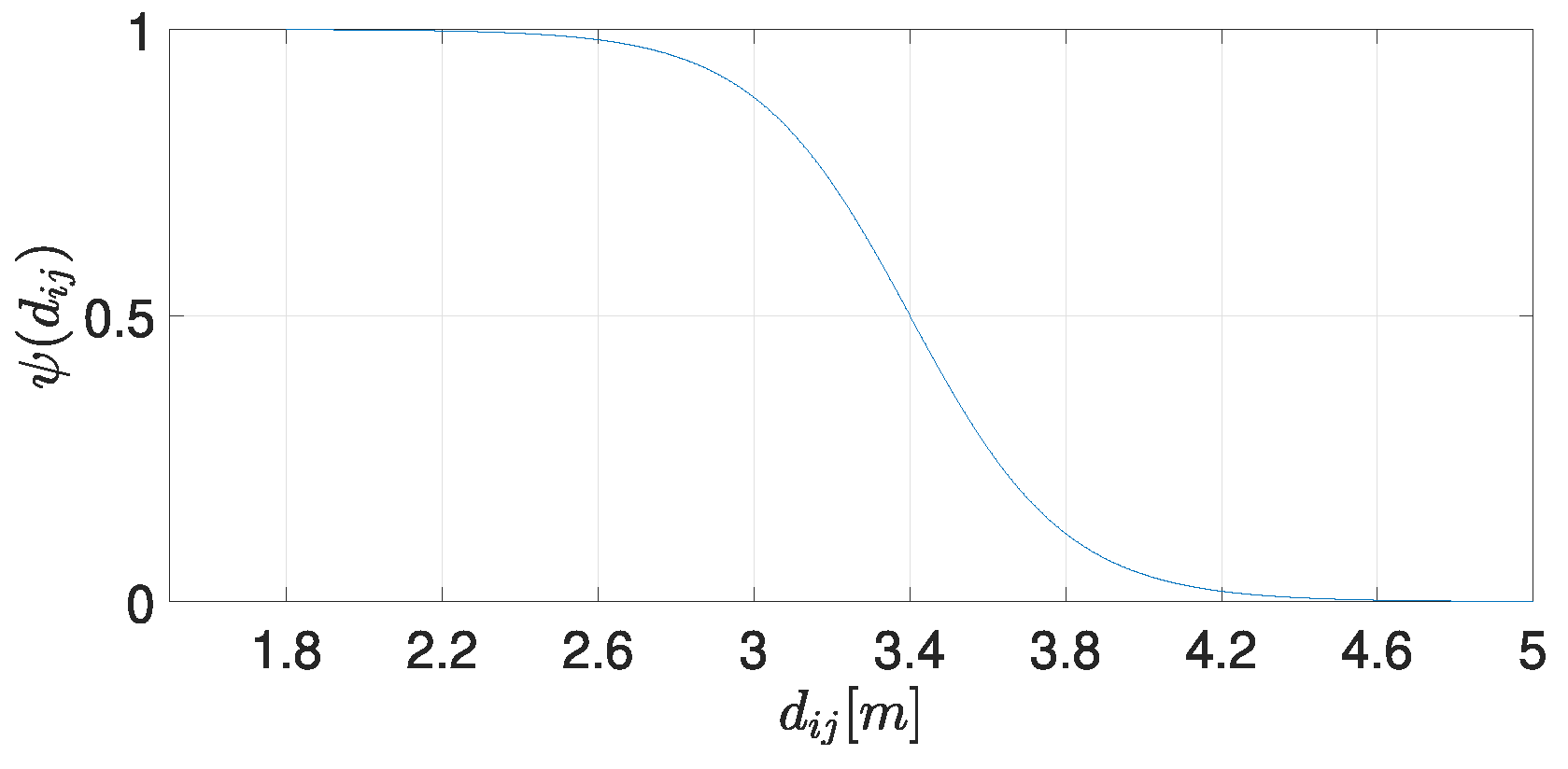
4.2. Collision Avoidance Strategy

Once the convergence to the desired formation has been shown, it is necessary to design a complementary strategy to guarantee collision-free motion by ensuring that the agents remain at a minimum predefined distance. Similar to the last subsection, we start with a proposal for a previously studied first-order system [40] that ensures collision-free performance. The basic strategy is given by the following:

$$u_i=-\mu \varphi \left({\tilde{z}}_i\right)-\epsilon \sum _{j=1,j\ne i}^N{\psi }_{ij}\left(d_{ij}\right)F\left[\begin{array}{c}{x}_j-x_i\\ y_j-y_i\end{array}\right],$$

(28)

where the second right-hand term provides a repulsive action in the form of an unstable focus structure provided by the matrix:

$$F=\left[\begin{array}{cc}1& -1\\ 1& 1\end{array}\right].$$

(29)

The repulsive component is activated in a smooth way using the distance-based switching function ${\psi }_{ij}(·)$, which takes values between 0 and 1 as the distance between the i-th and the agent j-th goes from D to d. The parameter $ϵ$ is a positive constant that guarantees collision-free motion for values $ϵ={\displaystyle \frac{2\mu }{d}}$ ([42]). If we apply (28), the position error dynamics (12) are as follows:

$$\dot{\tilde{z}}=-\mu \left({\Delta }^{-1}\mathcal{L}\left(G\right)\otimes I_2\right)\varphi \left(\tilde{z}\right)+\epsilon \left({\Delta }^{-1}\mathcal{L}\left(G\right)\otimes I_2\right)\left(\Omega \otimes F\right)z,$$

(30)

where $\Omega$ is a matrix that depends on the distance between every pair of agents and models the conflicts among agents. Its general form is as follows:

$$\Omega =\left[\begin{array}{cccc}\sum _{j=1,j\ne i}^N\psi \left(d_{1j}\right)& -\psi \left(d_{12}\right)& \dots & -\psi \left(d_{iN}\right)\\ -\psi \left(d_{21}\right)& \sum _{j=1,j\ne i}^N\psi \left(d_{2j}\right)& \dots & -\psi \left(d_{2N}\right)\\ ⋮& \ddots & & ⋮\\ -\psi \left(d_{N1}\right)& -\psi \left(d_{N2}\right)& \dots & \sum _{j=1,j\ne i}^N\psi \left(d_{Nj}\right)\end{array}\right].$$

(31)

Remark 2.

It is important to note that (30) is reduced to (14) when the agents are far away from each other, that is, there is no risk of collision between any pair of agents. Then, the second right-hand term in (30) could be considered a vanishing perturbation term at the origin of the stable dynamics (14).

Assumption 1.

The intended configuration is specified such that the separation between any two agents exceeds a predefined minimum d, ensuring that no agent falls within another’s sensing range. In the same way, we assume that under the initial conditions, there exists no risk of collision between agents, that is, $\parallel z_i\left(0\right)-z_j\left(0\right)\parallel >d$, $\forall i,j\in N$.

If we proceed as in the previous subsection, we can define an auxiliary variable such that we have the following:

$$\dot{\tilde{z}}=-\mu \left({\Delta }^{-1}\mathcal{L}\left(G\right)\otimes I_2\right)\varphi \left(\tilde{z}\right)+\left({\Delta }^{-1}\mathcal{L}\left(G\right)\otimes I_2\right)\zeta +\beta \left(z\right),$$

(32)

where $\beta \left(z\right)=\epsilon \left({\Delta }^{-1}\mathcal{L}\left(G\right)\otimes I_2\right)\left(\Omega \otimes F\right)z$ and $\zeta =\mu \varphi \left(\tilde{z}\right)+v-\epsilon \left(\Omega \otimes F\right)z$. This auxiliary variable has dynamics, as follows:

$$\dot{\zeta }=\mu {\left({\displaystyle \frac{\partial \varphi \left(\tilde{z}\right)}{\partial \tilde{z}}}\right)}^T({\Delta }^{-1}\mathcal{L}\left(G\right)\otimes I_2)v+u+{\omega }^T\theta -\epsilon \left(\dot{\Omega }\otimes F\right)z-\epsilon \left(\Omega \otimes F\right)v.$$

(33)

At this point, we need to note that, indeed, the repulsive component of the control law imposes changes in the trajectory followed by the agents. Then, to distinguish the effect of the repulsive vector field provoked by the presence of surrounding agents from the local parametric uncertainty, the adaptation law is applied only when there is no risk of collision, that is, when no agents are detected in the sensing region. Otherwise, the control law regarding the repulsive component is implemented using the last estimated parameters until the conflict between agents is solved. Therefore, the control input can be chosen as follows:

$$u=-\mu {\left({\displaystyle \frac{\partial \varphi \left(\tilde{z}\right)}{\partial \tilde{z}}}\right)}^T({\Delta }^{-1}\mathcal{L}\left(G\right)\otimes I_2)v-{\omega }^T\overline{\theta }+\epsilon \left(\dot{\Omega }\otimes F\right)z+\epsilon \left(\Omega \otimes F\right)v-\lambda \zeta ,$$

(34)

where $\lambda >0$ and $\overline{\theta }$ are the last estimations of the vector $\theta$, giving priority to the safety motion over the formation control objective. Once the conflict between agents has been solved, the agents restart the parameter adaptation. We are now ready to state our main result.

Theorem 2.

Consider the closed-loop system (12)–(13) and the control law (34) along with definitions (29) and (31). Consider that the formation graph contains at least a directed spanning tree, and Assumption 1 holds. If there is no risk of collision among agents, the control law (34) becomes (21) where the estimated vector $\widehat{\theta }$ is obtained from the adaptation law:

$$\dot{\widehat{\theta }}=\Gamma w\zeta$$

(35)

where $\Gamma >0$ is a definite positive matrix in $R^{2N\times 2N}$. On the other hand, if there is a pair of agents entering their sensing region, the control law (34) is applied using $\overline{\theta }$, which is the last estimated value of θ. Then, mobile agents are able to resolve any conflict between them and reach the desired formation while compensating for their local uncertainty. Moreover, the velocity of the formation becomes zero once the formation pattern has been achieved.

Proof. 

As mentioned, when agents are far enough from each other, the applied control law is (21), which corresponds to Theorem 1. Then, it is necessary to show that when agents are at risk of collision, strategy (34) is able to effectively solve conflicts to prevent collisions. In the closed-loop system, we have the following:

$$\begin{array}{ccc}\hfill \dot{\tilde{z}}& =& -\mu ({\Delta }^{-1}\mathcal{L}\left(G\right)\otimes I_2)\varphi \left(\tilde{z}\right)+\beta \left(z\right)+({\Delta }^{-1}\mathcal{L}\left(G\right)\otimes I_2)\zeta \hfill \end{array}$$

(36)

$$\begin{array}{ccc}\hfill \dot{\zeta }& =& -\lambda \zeta -{\omega }^T{\theta }_{\Delta },\hfill \end{array}$$

(37)

where ${\theta }_{\Delta }=\overline{\theta }-\theta$ is the estimation error, which is constant, while the collision avoidance component is applied. Since there is no adaptation law, we just use a single quadratic Lyapunov function, as follows:

$$V_2={\displaystyle \frac{1}{2}}{\zeta }^T\zeta$$

whose time derivative is as follows:

$${\dot{V}}_2={\zeta }^T\dot{\zeta }=-\lambda {\zeta }^T\zeta -{\zeta }^T{\omega }^T{\theta }_{\Delta }.$$

If $\omega$ is bounded by $\parallel \omega \parallel \le k\parallel \zeta \parallel$, then we have the following:

$${\dot{V}}_2\le -{\lambda \parallel \zeta \parallel }^2+k\parallel {\theta }_{\Delta }{\parallel \parallel \zeta \parallel }^2\le -(\lambda -k\parallel {\theta }_{\Delta }{\parallel )\parallel \zeta \parallel }^2,$$

which implies that $\parallel \zeta \parallel \to 0$ when $\lambda >k\parallel {\theta }_{\Delta }\parallel$. Then, (36) is input-to-state stable, which in combination with ensures that $\tilde{z}\to 0$. As a result, we have the following:

$$\parallel v\parallel +\parallel \beta \left(z\right)\parallel \to 0$$

As mentioned before, $\beta \left(z\right)$ is a vanishing perturbation at the origin of the subsystem, then $\parallel \beta \left(z\right)\parallel \to 0$, which finally means that $\parallel v\parallel \to 0$. In summary, the agents reach the desired formation while they avoid collisions. In addition, the whole formation remains static after it is achieved. □

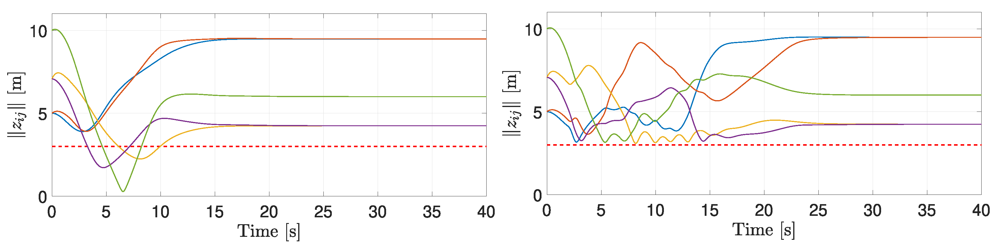
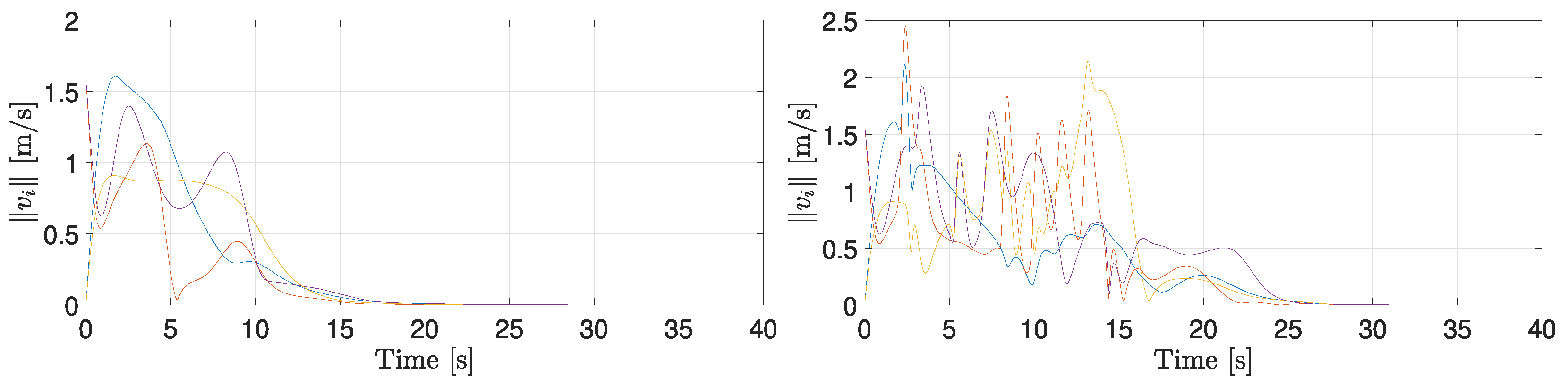
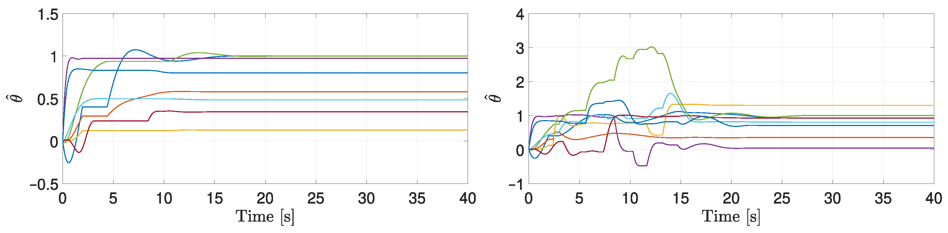
5. Simulation Results

In this section, we present the results of numerical simulations carried out to show the performance of the proposed scheme. The first one consists of a reduced system composed of only two agents and is meant to illustrate as clearly as possible the main features of our scheme. Then, a second simulation was developed with the objective of verifying the performance of our strategy in a more complex scenario composed of four agents.

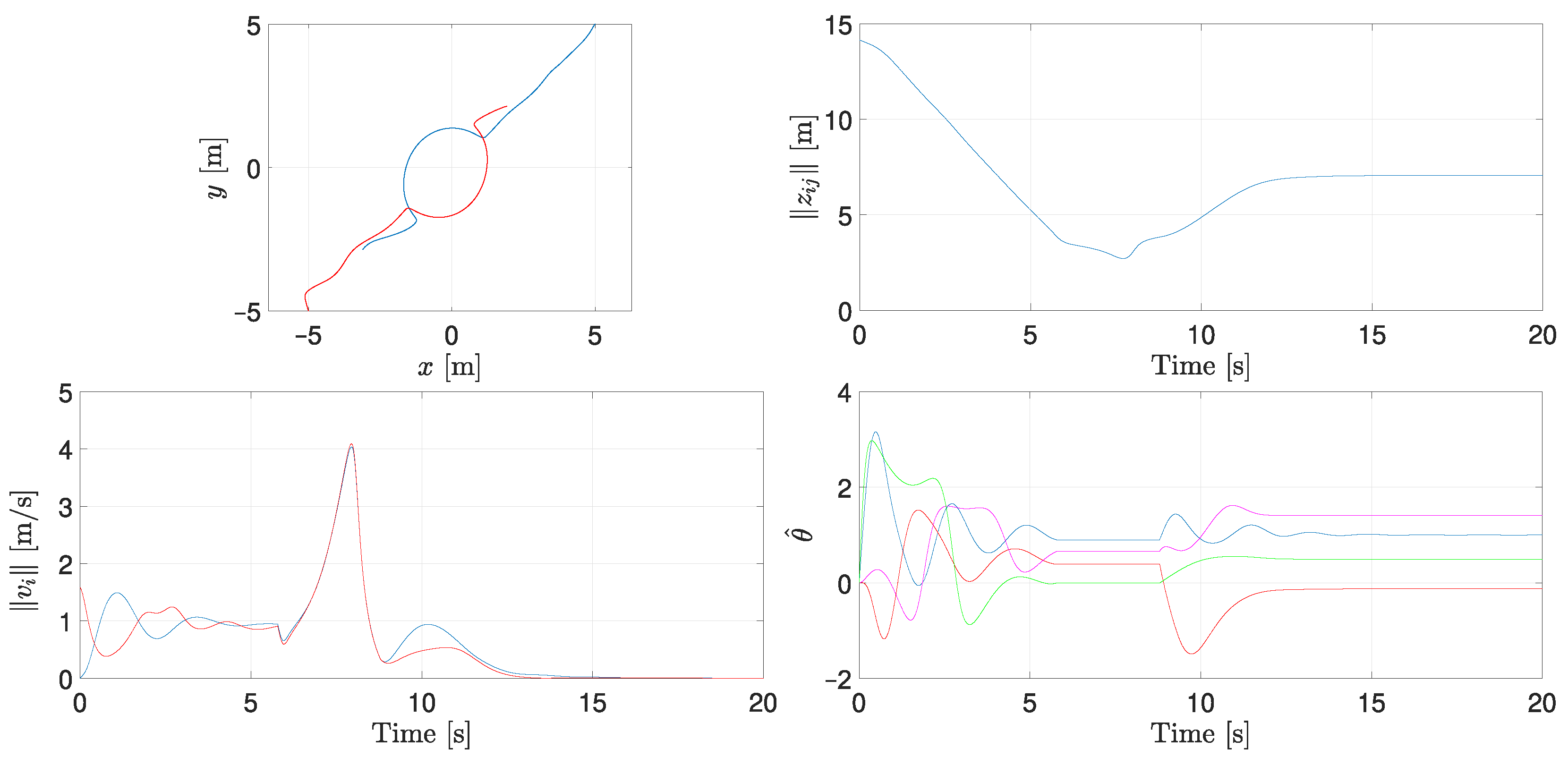
5.1. Two-Agent System with Bidirectional Communication

Consider a pair of second-order agents in the plane with linearly parameterized uncertainty:

$$\begin{array}{ccc}\hfill {\dot{z}}_1& =& v_1\hfill \\ \hfill {\dot{v}}_1& =& u_1+\left[\begin{array}{cc}0& sin{v}_{1_y}\\ cos{v}_{1_x}& 0\end{array}\right]\left[\begin{array}{c}1\\ 0.5\end{array}\right],\hfill \end{array}$$

$$\begin{array}{ccc}\hfill {\dot{z}}_2& =& v_2\hfill \\ \hfill {\dot{v}}_2& =& u_2+\left[\begin{array}{cc}{v}_{2_x}sint& 0\\ 0& v_{2_y}cost\end{array}\right]\left[\begin{array}{c}0.7\\ 0.3\end{array}\right],\hfill \end{array}$$

with $v_i={[v_{i_x},v_{i_y}]}^T$, $i=1,2$. Assume there is bidirectional communication between the agents, and the objective is for them to be positioned at specific locations relative to each other. This displacement is given by the constant vector $c_{21}=-c_{12}={[-3,-3]}^T$. The initial conditions are $z_1\left(0\right)={[5,5]}^T$, $z_2\left(0\right)={[-5,-5]}^T$, $v_1\left(0\right)={[0,0]}^T$, and $v_2\left(0\right)={[-1,2]}^T$. The function used to apply the repulsive component is given by the following:

$$\psi \left(d_{ij}\right)={\displaystyle \frac{1}{1+e^{b(d_{ij}-a)}}}$$

with values $a=3.4$ and $b=5$. As we can see in Figure 1, the switching function is fully activated for distances of about $2.2$ m.

It is important to note that the initial positions were selected to provoke an imminent risk of collision. In the same way, initial estimated parameters were assumed to be zero, which means that there was no prior knowledge of real values. The results of this first simulation are shown in Figure 2, where, in the upper left corner, the trajectories of the agents in the plane are shown. It is clear that the agents reach the desired relative positions while they avoid the collision successfully and do not become stuck even when applying the same vector field. Moreover, they exhibit smooth behavior given by the transition and saturation functions involved in the control law. In the upper right corner, the distance between the agents is depicted. As can be seen, the distance never decreases more than the safety distance. The magnitudes of the velocities are shown in the lower left corner, while the estimated parameters are depicted in the lower right corner. The period from 6 to 8 s, during which the estimated parameters remain constant, corresponds to when the parameter estimation is frozen to prioritize collision avoidance control.

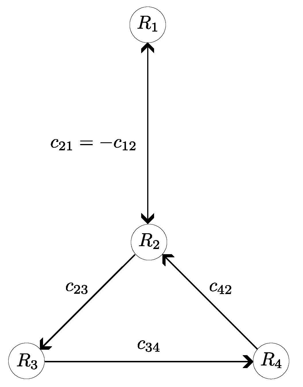
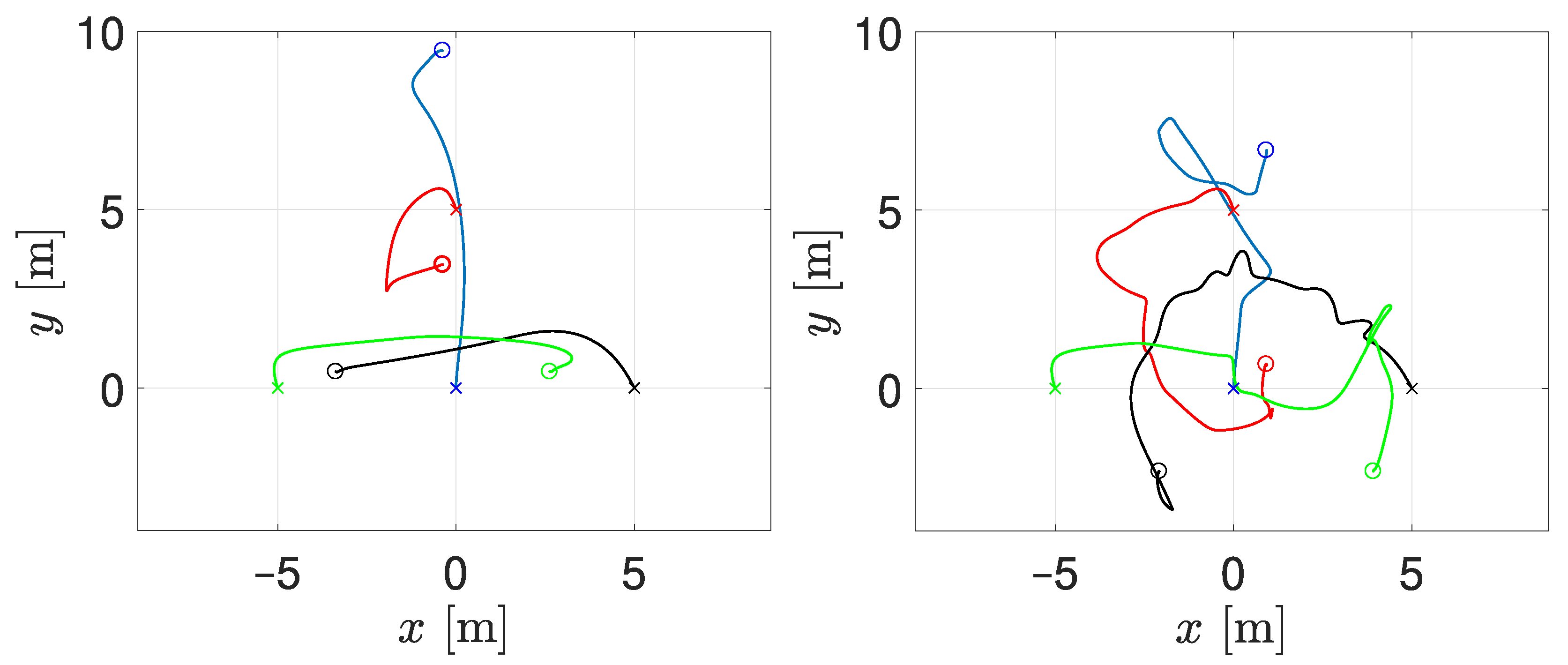
5.2. Four-Agents System with General Communication Topology

As a second example, consider a set of four agents whose communication graph is shown in Figure 3. The geometric pattern to be formed is defined by the constant vectors $c_{21}=-c_{12}={[0,2\ell ]}^T$, $c_{23}={[-\ell ,-\ell ]}^T$, $c_{34}={[2\ell ,0]}^T$, $c_{42}={[-\ell ,\ell ]}^T$, $\ell =3$. For this simulation, we consider agents with a similar local uncertain term as in the previous example, i.e., we have the following:

$$\begin{array}{ccc}\hfill {\dot{z}}_i& =& v_i\hfill \\ \hfill {\dot{v}}_i& =& u_i+\left[\begin{array}{cc}0& sin{v}_{i_y}\\ cos{v}_{i_x}& 0\end{array}\right]\left[\begin{array}{c}1\\ 0.5\end{array}\right],\hfill \end{array}$$

for $i=1,3$, and for $i=2,4$, we have the following:

$$\begin{array}{ccc}\hfill {\dot{z}}_i& =& v_i\hfill \\ \hfill {\dot{v}}_i& =& u_i+\left[\begin{array}{cc}{v}_{i_x}sint& 0\\ 0& v_{i_y}cost\end{array}\right]\left[\begin{array}{c}0.7\\ 0.3\end{array}\right].\hfill \end{array}$$

For the switching function, parameters were $a=3.6$ and $b=10$, which fully activate the repulsive force at about 3 meters. The initial conditions were $z_1\left(0\right)={[0,0]}^T$, $z_2\left(0\right)={[0,5]}^T$, $z_3\left(0\right)={[5,0]}^T$, $z_4\left(0\right)={[0,5]}^T$, $v_1\left(0\right)={[0,0]}^T$, $v_2\left(0\right)={[-0.5,1.5]}^T$, $v_3\left(0\right)={[0,0]}^T$, $v_4\left(0\right)={[-0.5,1.5]}^T$. In Figure 4, Figure 5, Figure 6 and Figure 7, the results of this simulation are shown, comparing the behavior of the system under the control laws with and without repulsive vector fields on the left and right, respectively. Figure 4 illustrates the trajectories of the agents in the plane, verifying that—in both cases—the desired formation is reached. However, in Figure 5, the distances between each pair of agents are shown; it is clear that when applying the avoidance component, the agents remain at a greater distance than the safety radius. On the other hand, Figure 6 shows that in both cases the velocity of the resulting formation becomes zero, but the settling time is larger if the collision avoidance strategy is applied. Finally, in Figure 7, local estimated parameters are depicted. In this case, when there exists a conflict between any pair of agents, the estimation law is stopped, and the last estimated value is used to apply the control input. When agents become separated, the adaptation law is re-established.

6. Conclusions

In this paper, we proposed an adaptive strategy to solve the formation control problem for a set of second-order agents with parametric uncertainty. Repulsive vector fields with an unstable focus structure were used to avoid collisions among agents by keeping them at a distance greater than or equal to a predefined minimum bound. These vector fields are such that the agents do not become stuck in any undesired configuration while repelling each other. The adaptation law is applied only when there is no risk of collisions, while the controller keeps and uses the last estimated parameter in the control law until the conflict between agents is solved, and then the adaptation continues in order to ensure the desired position is reached despite the uncertainty. Simulations were carried out to illustrate the performance of the proposed algorithm, which shows the effectiveness of the approach. As the next step, time-varying formation tracking, connectivity preservation, and communication delay could be considered, as well as experimental validation.

References

1. Jawhar, I.; Mohamed, N.; Kesserwan, N.; Al-Jaroodi, J. Networking Architectures and Protocols for Multi-Robot Systems in Agriculture 4.0. In Proceedings of the 2022 IEEE International Systems Conference (SysCon), Virtual, 25– 28 April 2022; pp. 1–6. [Google Scholar] [CrossRef]
2. Huang, L.; Zhou, M.; Hao, K.; Han, H. Multirobot Cooperative Patrolling Strategy for Moving Objects. IEEE Trans. Syst. Man Cybern. Syst. 2023, 53, 2995–3007. [Google Scholar] [CrossRef]
3. Noh, D.; Choi, J.; Choi, J.; Byun, D.; Kim, Y.; Kim, H.R.; Baek, S.; Lee, S.; Myung, H. MASS: Multi-Agent Scheduling System for Intelligent Surveillance. In Proceedings of the 2022 19th International Conference on Ubiquitous Robots (UR), Jeju, Republic of Korea, 4–6 July 2022; pp. 252–257. [Google Scholar] [CrossRef]
4. Abusalama, J.; Alkharabsheh, A.R.; Momani, L.; Razali, S. Multi-Agents System for Early Disaster Detection, Evacuation and Rescuing. In Proceedings of the 2020 Advances in Science and Engineering Technology International Conferences (ASET), Dubai, United Arab Emirates, 4 February–9 April 2020; pp. 1–6. [Google Scholar] [CrossRef]
5. Queralta, J.P.; Taipalmaa, J.; Can Pullinen, B.; Sarker, V.K.; Nguyen Gia, T.; Tenhunen, H.; Gabbouj, M.; Raitoharju, J.; Westerlund, T. Collaborative Multi-Robot Search and Rescue: Planning, Coordination, Perception, and Active Vision. IEEE Access 2020, 8, 191617–191643. [Google Scholar] [CrossRef]
6. Olfati-Saber, R.; Fax, J.A.; Murray, R.M. Consensus and Cooperation in Networked Multi-Agent Systems. Proc. IEEE 2007, 95, 215–233. [Google Scholar] [CrossRef]
7. Chung, S.J.; Slotine, J.J.E. Cooperative Robot Control and Concurrent Synchronization of Lagrangian Systems. IEEE Trans. Robot. 2009, 25, 686–700. [Google Scholar] [CrossRef]
8. Mastellone, S.; StipanoviÄ, D.M.; Graunke, C.R.; Intlekofer, K.A.; Spong, M.W. Formation Control and Collision Avoidance for Multi-agent Non-holonomic Systems: Theory and Experiments. Int. J. Robot. Res. 2008, 27, 107–126. [Google Scholar] [CrossRef]
9. Abhijith, U.P.; Thomas, S. Cyclic Pursuit of mobile robots: A linear approach. In Proceedings of the 2017 IEEE International Conference on Signal Processing, Informatics, Communication and Energy Systems (SPICES), Kollam, India, 8–10 August 2017; pp. 1–5. [Google Scholar] [CrossRef]
10. Oh, K.K.; Park, M.C.; Ahn, H.S. A survey of multi-agent formation control. Automatica 2015, 53, 424–440. [Google Scholar] [CrossRef]
11. Carvalho Filho, J.G.N.D.; Carvalho, E.Á.N.; Molina, L.; Freire, E.O. The Impact of Parametric Uncertainties on Mobile Robots Velocities and Pose Estimation. IEEE Access 2019, 7, 69070–69086. [Google Scholar] [CrossRef]
12. Fabris, M.; Fattore, G.; Cenedese, A. Optimal time-invariant distributed formation tracking for second-order multi-agent systems. Eur. J. Control 2024, 77, 100985. [Google Scholar] [CrossRef]
13. Dong, X.; Li, Q.; Wang, R.; Ren, Z. Time-varying formation control for second-order swarm systems with switching directed topologies. Inf. Sci. 2016, 369, 1–13. Available online: https://www.sciencedirect.com/science/article/pii/S0020025516303826 (accessed on 20 April 2025). [CrossRef]
14. Zou, Y.; Wen, C.; Guan, M. Distributed adaptive control for distance-based formation and flocking control of multi-agent systems. IET Control Theory Appl. 2019, 13, 878–885. [Google Scholar] [CrossRef]
15. Zhi, H.; Chen, L.; Li, C.; Guo, Y. Leader-Follower Affine Formation Control of Second-Order Nonlinear Uncertain Multi-Agent Systems. IEEE Trans. Circuits Syst. II Express Briefs 2021, 68, 3547–3551. [Google Scholar] [CrossRef]
16. Cheng, X.; Huang, J.; Gao, T.; Wang, S.; Zhang, M. Distributed adaptive control of mobile robots with unknown parameters. In Proceedings of the 2023 35th Chinese Control and Decision Conference (CCDC), Yichang, China, 20–22 May 2023; IEEE: New York, NY, USA, 2023; Volume 5, pp. 2624–2629. [Google Scholar] [CrossRef]
17. Zhang, J.; Fu, Y.; Fu, J. Adaptive Finite-Time Optimal Formation Control for Second-Order Nonlinear Multiagent Systems. IEEE Trans. Syst. Man Cybern. Syst. 2023, 53, 6132–6144. [Google Scholar] [CrossRef]
18. Zhao, W.; Liu, H.; Lewis, F.L.; Wang, X. Data-Driven Optimal Formation Control for Quadrotor Team with Unknown Dynamics. IEEE Trans. Cybern. 2022, 52, 7889–7898. [Google Scholar] [CrossRef] [PubMed]
19. Zhao, W.; Liu, H.; Wan, Y.; Lin, Z. Data-Driven Formation Control for Multiple Heterogeneous Vehicles in Air-Ground Coordination. IEEE Trans. Control Netw. Syst. 2022, 9, 1851–1862. [Google Scholar] [CrossRef]
20. Parlangeli, G. Data-Driven Formation Control for Multi-Vehicle Systems Induced by Leader Motion. Algorithms 2024, 17, 514. [Google Scholar] [CrossRef]
21. Golmisheh, F.M.; Shamaghdari, S. Data-Driven Inverse Reinforcement Learning for Heterogeneous Optimal Robust Formation Control. IEEE Trans. Cybern. 2025, 55, 2024–2037. [Google Scholar] [CrossRef]
22. Yu, M.; Wang, H.; Xie, G.; Jin, K. Event-triggered circle formation control for second-order-agent system. Neurocomputing 2018, 275, 462–469. [Google Scholar] [CrossRef]
23. Wang, X.; Sun, S.; Xiao, F.; Yu, M. Dynamic event-triggered formation control of second-order nonholonomic systems. J. Syst. Eng. Electron. 2023, 34, 501–514. [Google Scholar] [CrossRef]
24. Li, Y.; Qu, F.; Tong, S. Observer-Based Fuzzy Adaptive Finite-Time Containment Control of Nonlinear Multiagent Systems with Input Delay. IEEE Trans. Cybern. 2021, 51, 126–137. [Google Scholar] [CrossRef]
25. Li, Y.; Zhang, J.; Tong, S. Fuzzy Adaptive Optimized Leader-Following Formation Control for Second-Order Stochastic Multiagent Systems. IEEE Trans. Ind. Inform. 2022, 18, 6026–6037. [Google Scholar] [CrossRef]
26. Lan, J.; Liu, Y.J.; Xu, T.; Tong, S.; Liu, L. Adaptive Fuzzy Fast Finite-Time Formation Control for Second-Order MASs Based on Capability Boundaries of Agents. IEEE Trans. Fuzzy Syst. 2022, 30, 3905–3917. [Google Scholar] [CrossRef]
27. Wu, W.; Li, Y.; Tong, S. Neural Network Output-Feedback Consensus Fault-Tolerant Control for Nonlinear Multiagent Systems with Intermittent Actuator Faults. IEEE Trans. Neural Netw. Learn. Syst. 2023, 34, 4728–4740. [Google Scholar] [CrossRef] [PubMed]
28. Mondal, A.; Bhowmick, C.; Behera, L.; Jamshidi, M. Trajectory Tracking by Multiple Agents in Formation with Collision Avoidance and Connectivity Assurance. IEEE Syst. J. 2018, 12, 2449–2460. [Google Scholar] [CrossRef]
29. Pang, Z.H.; Zheng, C.B.; Sun, J.; Han, Q.L.; Liu, G.P. Distance- And velocity-based collision avoidance for time-varying formation control of second-order multi-agent systems. IEEE Trans. Circuits Syst. II Express Briefs 2021, 68, 1253–1257. [Google Scholar] [CrossRef]
30. Mu, C.; Peng, J. Learning-Based Cooperative Multiagent Formation Control with Collision Avoidance. IEEE Trans. Syst. Man Cybern. Syst. 2022, 52, 7341–7352. [Google Scholar] [CrossRef]
31. Yang, Y.; Liu, Q.; Tan, H.; Shen, Z.; Wu, D. Collision-Free and Connectivity-Preserving Formation Control of Nonlinear Multi-Agent Systems with External Disturbances. IEEE Trans. Veh. Technol. 2023, 72, 9956–9968. [Google Scholar] [CrossRef]
32. Yu, Y.; Chen, C.; Guo, J.; Chadli, M.; Xiang, Z. Adaptive Formation Control for Unmanned Aerial Vehicles with Collision Avoidance and Switching Communication Network. IEEE Trans. Fuzzy Syst. 2024, 32, 1435–1445. [Google Scholar] [CrossRef]
33. Catellani, M.; Sabattini, L. Distributed Control of a Limited Angular Field-of-View Multi-Robot System in Communication-Denied Scenarios: A Probabilistic Approach. IEEE Robot. Autom. Lett. 2024, 9, 739–746. [Google Scholar] [CrossRef]
34. Palani, T.; Fukushima, H.; Izuhara, S. Collision Avoidance Control for Distributed Multi-Robot Systems Using Collision Cones and CBF-Based Constraints. In Proceedings of the 2024 IEEE Conference on Control Technology and Applications (CCTA), Newcastle upon Tyne, UK, 21–23 August 2024; pp. 787–792. [Google Scholar] [CrossRef]
35. Tang, J.; Lao, S.; Wan, Y. Systematic Review of Collision-Avoidance Approaches for Unmanned Aerial Vehicles. IEEE Syst. J. 2022, 16, 4356–4367. [Google Scholar] [CrossRef]
36. Kot, R. Review of Collision Avoidance and Path Planning Algorithms Used in Autonomous Underwater Vehicles. Electronics 2022, 11, 2301. [Google Scholar] [CrossRef]
37. Lyu, H.; Hao, Z.; Li, J.; Li, G.; Sun, X.; Zhang, G.; Yin, Y.; Zhao, Y.; Zhang, L. Ship Autonomous Collision-Avoidance Strategies—A Comprehensive Review. J. Mar. Sci. Eng. 2023, 11, 830. [Google Scholar] [CrossRef]
38. Khalil, H.K. Nonlinear Systems, 3rd ed.; Prentice-Hall: Upper Saddle River, NJ, USA, 2002. [Google Scholar]
39. Slotine, J.; Li, W. Applied Nonlinear Control; Prentice-Hall International Editions; Prentice-Hall: Upper Saddle River, NJ, USA, 1991. [Google Scholar]
40. Flores-Resendiz, J.F.; Aranda-Bricaire, E. A General Solution to the Formation Control Problem Without Collisions for First-Order Multi-Agent Systems. Robotica 2020, 38, 1123–1137. [Google Scholar] [CrossRef]
41. Flores-Resendiz, J.F.; Avilés, D.; Aranda-Bricaire, E. Formation Control for Second-Order Multi-Agent Systems with Collision Avoidance. Machines 2023, 11, 208. [Google Scholar] [CrossRef]
42. Flores-Resendiz, J.F.; Aranda-Bricaire, E.; González-Sierra, J.; Santiaguillo-Salinas, J. Finite-Time Formation Control without Collisions for Multiagent Systems with Communication Graphs Composed of Cyclic Paths. Math. Probl. Eng. 2015, 2015, 948086. [Google Scholar] [CrossRef]
Figure 1. Switching function. The parameters a = 3.4 and b = 10 ensure a sensing region radius of about 4.6 meters and an avoidance safety distance of about 2.2 m.
Electronics 14 01751 g001
Figure 2. Simulation results for the two-agent system. (Upper left): trajectories of agents in the plane. (Upper right): distance between agents. (Lower left): velocities of agents. (Lower right): estimated parameters.
Electronics 14 01751 g002
Figure 3. Desired formation for the four-agent system. General communication graph with only one undirected edge, while the rest of the edges are directed.
Electronics 14 01751 g003
Figure 4. Trajectories of agents in the plane without collision avoidance component (left) and and with the application of the repulsive component (right).
Electronics 14 01751 g004
Figure 5. Distances between any pair of agents in the plane without collision avoidance component (left) and with the application of the repulsive component (right).
Electronics 14 01751 g005
Figure 6. Velocities of agents without the collision avoidance component (left) and with the application of the repulsive component (right). It is worth noting that—in both cases—the formation remains stationary after reaching the desired geometric pattern.
Electronics 14 01751 g006
Figure 7. Estimated parameters for both cases, without the collision avoidance component (left) and with the application of the repulsive component (right).
Electronics 14 01751 g007
Disclaimer/Publisher’s Note: The statements, opinions and data contained in all publications are solely those of the individual author(s) and contributor(s) and not of MDPI and/or the editor(s). MDPI and/or the editor(s) disclaim responsibility for any injury to people or property resulting from any ideas, methods, instructions or products referred to in the content.