Abstract
Conventional matched-field processing (MFP) for acoustic source localization is sensitive to environmental mismatches because it is based on the wave propagation model and environmental information that is uncertain in reality. In this paper, a mode-predictable sparse Bayesian learning (MPR-SBL) method is proposed to increase robustness in the presence of environmental uncertainty. The estimator maximizes the marginalized probability density function (PDF) of the received data at the sensors, utilizing the Bayesian rule and two hyperparameters (the source powers and the noise variance). The replica vectors in the estimator are reconstructed with the predictable modes from the decomposition of the pressure in the representation of the acoustic normal mode. The performance of this approach is evaluated and compared with the Bartlett processor and original sparse Bayesian learning, both in simulation and using the SWellEx-96 Event S5 dataset. The results illustrate that the proposed MPR-SBL method exhibits better performance in the two-source scenario, especially for the weaker source.
1. Introduction
MFP is a generalized beamforming method which matches the signals received at a vertical line array (VLA) with replica vectors to localize the sources in range and in depth [1]. The exact localization of the MFP method depends on the accurate calculation of the replica vectors, which are calculated based on the wave propagation model and the known environmental information. In practice, the spatial and the temporal variations in underwater environmental parameters, such as the speed profile, the properties of the sediments, and the water depth, cause severe performance degradation of the localization. If there exists an environmental mismatch, the results of the conventional MFP methods tend to have serious side lobe errors, which confuse the estimation of the true source’s position.
Overcoming the performance degradation caused by environmental mismatch in MFP is an attractive and challenging research topic. Many methods have been developed surrounding this topic. They can be generally classified into three categories: variants of MFP based on a posteriori probability [2,3], multiple constraint processors [4,5] and matched mode processing (MMP) [6,7,8,9,10]. In the first kind of MFP-like algorithms, the approaches take the uncertain environmental parameters as random variables. The localization is completed by maximizing a posterior PDF, an integration of the product of the observation’s PDF and the prior densities of the uncertainty over these variables. The major disadvantage of these methods is that a great deal of computation time is required when performing an integration operation over the space of these perturbed environmental parameters. The algorithms belonging to the second category, such as the multiple constraint method (MCM) [4] and minimum variance beamformers with environmental perturbation constraints (MV-EPC) [5], require the replica vectors (the optimal weight vector) to satisfy a set of constraints in order to solve the uncertainty. In comparison to the former methods, they have a low low computation cost, but their robustness to environmental mismatch is not satisfactory in general mismatch cases [11] where uncertainty exists relating to the sound speed, sediment, and water depth. As an alternative method to MFP, MMP matches the modal amplitudes decomposed from the received pressure field data with those obtained from the replica field. It often selects the modes by ignoring higher and/or lower order modes, which are assumed to be less sensitive to environmental mismatch in order to reduce the performance degradation. However, MMP has difficulty in accurately estimating all the modal amplitudes, especially at low signal-to-noise ratios (SNRs). To improve the performance of MMP-like algorithms, Tabrikian et al. [12] proposed a robust maximum-likelihood estimator which is based on the entire modal amplitude from the predictable modes and the modal depth eigenfunctions at the array from the unpredictable modes instead of directing using the received data of the array. The predictable modes are assumed to be less sensitive to the environmental mismatch, whereas the unpredictable ones are more sensitive to the mismatch. In the general mismatch environment, the modes whose orders are from 3 to 9 are selected as predictable modes, which means the lower and higher order modes are ignored while the middle order modes remain. The results of these experiments illustrate that this processor achieves a significant performance improvement compared to that of the classical MMP when dealing with mismatches.
Recently, an sparse Bayesian learning (SBL) algorithm was proposed for source localization in underwater acoustics. It has less side lobes and exhibits better performance in localizing a weaker source in a two-source scenario, in contrast to the conventional Bartlett processor [13]. However, its robustness to environmental mismatches, such as errors in sound-speed profile, water depth, and properties of sediment, is poor. Therefore, in this paper, a mode-predictable based SBL (MPR-SBL) method is proposed to provide a robust solution to environmental mismatching.
The rest of the paper is organized as follows: a detailed description of MPR-SBL algorithm is provided in Section 2. In Section 3, the performance of the MPR-SBL is illustrated by simulations and at-sea experiment results. In addition, the non-adaptive Bartlett and the classical SBL algorithm are provided as comparative methods. We draw a conclusion in Section 4.
2. Mode-Predictable Based Sparse Bayesian Learning
In this section, we specifically introduce the proposed MPR-SBL algorithm. It is composed of two subsections. First, the signal model is established in Section 2.1, which utilizes the reconstructed replica vectors calculated in Section 2.2. Secondly, we describe how to decompose the acoustic field into predictable and unpredictable subspaces of the normal mode representation and the calculation of the reconstructed replica vectors with the predictable modes (Section 2.2). Finally, the SBL processor is introduced based on the signal model in Section 2.3.
2.1. Signal Model
The signal emitted by the K acoustic sources is received at a vertical linear array (VLA) composed of N receivers at a single frequency. For L snapshots, the received signals are expressed as . The propagation process is modeled by an under-determined system of the linear equations as follows.
where is the replica dictionary whose column vector represents the calculated replica vector at the positions of VLA when a source is located at . The superscript T indicates transposition. D represents the number of grid points within the search domain, where . represents a pair of parameters where is the dth possible source’s range vertical to the VLA and is the same source’s depth beneath the ocean surface. describes the the complex source amplitudes of the received signal. The column vector is defined as , whose element corresponds to the dth position and the lth snapshot. is assumed as complex Gaussian noise with variance . Because the replica vectors are accumulated by several modes, which could be divided into predictable modes and unpredictable modes (details in Section 2.2), can be decomposed as follows:
where is composed of the pressures produced by the predictable modes, while is composed of those produced by the unpredictable ones. Therefore, the linear equation (Equation (1)) is rewritten as:
where is taken as generalized environmental noise [14] and it satisfies the complex Gaussian distribution with variance . represents the reconstructed replica vectors.
2.2. The Calculation of the Reconstructed Replica Vectors
The pressure of a source at the position () of the acoustic field can be represented as the summation of the modes in the normal modal representation:
where is the water density at the source depth ; is the bth mode depth amplitude as a function of depth; and is the corresponding horizontal wave number.
In a shallow-water waveguide, different kinds of modes experience different kinds of propagations, which means that they have different responses to the environmental mismatch. Some modal amplitudes remain more correlated than others in the presence of the environmental mismatch. That is to say, the available information contained in those modes about the source position is stronger than that which exists in other modes. On the other hand, the higher-order modes corresponding to rays that reflect more times from the boundaries and delay longer in the medium are more easily affected by the boundary interaction, which is one of the main uncertainties in the acoustic propagation model. Therefore, the uncertain variations in the medium and boundaries affect more in the higher-order modes than the lower-order ones, which results in less correlation between the higher-order modes, providing less useful information on source location. In this paper, those having more correlation with source information and higher SNRs are assumed to be the predictable modes, while the others are assumed to be the unpredictable ones.
In order to find the predictable modes, the environmental variations are assumed as random variables. The errors in the replica field caused by the environmental mismatch can be reflected in the errors of both the modal horizontal wave number and the eigenfunctions . The errors of modal horizontal wave numbers have more influence on the estimation than the modal eigenfunctions because the source range tends to be much larger than the channel depth in shallow water and the phase is the product of the and the range. Based on the variations in the horizontal wave number and the eigenfunctions of normal modes, it is possible to assess the impact of environmental mismatches on these waves. The predictable modes are identified through normal mode decomposition [15,16], which involves decomposing the acoustic field (as illustrated in Equation (4)) into a predictable subspace and an unpredictable one. This process aims to identify the normal modes that are least affected by environmental mismatches [12].
To evaluate the correlation of the modes, the second order statistics of the horizontal wave numbers are computed. groups of modes are generated by a normal mode propagation model program, KRAKEN [17], utilizing independent random realizations of the uncertain parameters.
Assuming a candidate group with modes selected from all the B modes, a modal horizontal wave number vector is formed to calculate its covariance matrix :
where , as the unbiased estimator of the mean of , represents , and , is the th realization. In total, groups need to be calculated to find the best selection, where is the factorial of B.
To observe the effects of the errors on the horizontal wave number vector , we decompose :
where is a vector of one. Defining a matrix , the vector is orthogonal to . Thus, is given by:
where .
While the errors in the subspace of , and , result in a bias, respectively, in the source range estimate and the complex signal amplitude estimate, the other errors caused by result in distortions of the ambiguity/likelihood function [12]. As it is assumed that the unpredictable modes cause the error , they should be excluded. Thus, the covariance matrix is projected into the null space of the matrix , as shown in Equation (8).
In order to find the set of the predictable modes , we minimize the trace of , which represents the minimization of the variability of :
where is the combination of all the -sized subsets of the B modes, and is defined as one of these subsets. Thus, is the covariance matrix with horizontal wave numbers in the particular subset .
Because the mode-based pressure is calculated by several modes (Equation (4)), the reconstructed replica matrix is accumulated through . The element in the matrix , represents the pressure at the nth sensor if there is a source at the dth position. Hence, the matrix is expressed as:
2.3. Processor
The vector of complexity signal amplitudes, , is sparse because only a few of entries in the vector are nonzero for the number of true sources . Thus, assuming satisfies a zero-mean complex Gaussian distribution, the prior probability density is given, where is a diagonal covariance matrix and () denotes the source energy at the site of . The prior of can be computed as follows:
Due to the fact that the noise is Gaussian with variance , the likelihood of for a given is obtained in Equation (12).
where is a N-dimensional identify matrix. Thus, the PDF of is computed as follows:
The hyperparameters and are estimated through a type- maximum likelihood and maximizing the PDF in Equation (13):
where
is the covariance of the received data and and represent the estimates of the hyperparameters and , respectively. means the determinant of a matrix.
The equation above (Equation (14)) is derived by the elements to obtain iterator [13]:
where is defined as 2-norm of a vector.
The estimation of is derived from the Equation (15) [18]:
where is the Moore-Penrose pseudo-inverse of the matrix , and is the sample covariance matrix (SCM). The active set comprises the indices of the nonzero elements of , which can be derived from the K strongest peaks of . This information serves as an estimate for the source location. The number of , K is assumed as the estimated number of the source, but the true one is not limited by it because the performance of SBL is not sensitive to K [13]. represents the column of corresponding to .
3. Simulations and Experiments
In this section, the performance of the proposed SBL is tested using simulations and the SWellEx-96 Event S5 dataset [13,19]. For environmental mismatches, this proposed method is evaluated and compared with the conventional Bartlett processor, a robust Bartlett processing (MPR-Bartlett) [14] algorithm, and the original SBL [13] through a Monte Carlo performance analyses.
3.1. Scenarios
Two scenarios considered in these tests are illustrated in Figure 1. Figure 1a shows a general mismatch case (genlmis) [11] and Figure 1b shows a range-independent waveguide geo-acoustic model of real data. The genlmis scenario as a benchmark model was provided in a workshop held in 1993 at the Naval Research Laboratory for mismatching tests. Specific parameters are shown in Table 1. The receiving array in this scenario is a VLA composed of 20 array elements, which are evenly distributed in the water from 5 m to 100 m, and the array elements are separated by 5 m. The frequency of this scene is set to 250 Hz.
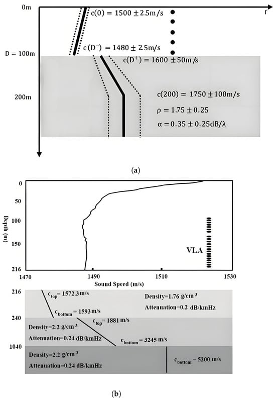
Figure 1.
Two range-independent acoustic models of shallow-water waveguide in simulations: (a) A conventional mismatch scene (genlmis), which is divided into three layers from top to bottom: water layer, sediment layer, and half space; (b) SWellEx-96 acoustic model of shallow sea waveguide, which is divided into four layers from top to bottom: water layer, sediment layer, mudstone layer, and half space. The gray part of the first layer indicates the range of sound velocity.

Table 1.
The parameters of uncertain shallow-water environment in genlmis scenario.
The SWellEx-96 experiment was conducted near the tip of Point Loma near San Diego, CA, USA. A ship, R/V Sproul, traveled 12 km at a speed of 2.5 m/s, towing shallow and deep sources at about 10 m and 60 m depth, respectively. The acoustic sources transmitted various broadband and multiple signals, received by a 21-element VLA at a sampling frequency of 1500 Hz. In this paper, the signal of the deep source at the frequency 166 Hz is used for processing. The scenario in Figure 1b provides an environmental profile of the SWellEx-96 Event S5 data. In this scenario, the receiving array VLA covers a depth of m to m, with an array element interval of m, and a total of 22 array elements. The data on the eighth sensor located at a depth of m was ignored because of some problems with this particular sensor. A total of 51 conductivity, temperature, and depth (CTD) profiles were recorded during the sea trial experiment, corresponding to the depth and sound velocity at different times and locations. Therefore, there are errors in the measured environmental parameters. In this paper, the “i9605.prn” sound velocity configuration is chosen for examination, because the measurement was closest to the dragging activity of the sound source in time and space. Based on this configuration and the original waveguide model, an environmental mismatch scene is constructed (Table 2). In water, the range of sound velocity is m/s, where c is the sound velocity recorded in the sound velocity profile, and it is assumed that the sound velocity value represents a random number within the range of . Other parameter values also change around the real environmental values.
Table 2.
The parameters of uncertain shallow-water environment in SWellEx-96 scenario.
According to the genlmis mismatch environment parameters in Table 1 and the self-defined mismatch environment parameters of SWellEx-96 in Table 2, the corresponding predictable normal waves are calculated by using Equation (9). Meanwhile, the acoustic field modeling, when combined with various uncertain environmental parameters simultaneously, can be represented by the Equation (4). In the experiments described in this paper, the acoustic field dataset is generated using KRAKEN [17]. KRAKEN is a specialized software for acoustic field calculations based on mode theory, which accepts all mismatched environmental parameters listed in Table 1 and Table 2 as input. This approach effectively integrates all relevant environmental parameters into the corresponding acoustic field data. We set the number of random environments to be equal to 100. In the genlmis mismatch scenario, the predictable normal wave sequence numbers are 3 to 9, and in the SWellEx-96 mismatch scenario, the predictable normal wave sequence numbers are 1 to 14. At the same time, the program is used to generate the replica vectors of the corresponding scene based on the assumed values in Table 1 and Table 2. In the genlmis scene, the search space ranges from 2 m to 100 m in depth and 2 m in interval, and from 0.05 km to 10 km in range and 50 m in interval. In the SWellEx-96 scene, the depth of the search space ranges from 10 m to 200 m with intervals of 10 m, while the range ranges from 0.05 km to 10 km with intervals of 50 m. In addition, the array tilt is set to 1 degree, because the VLA was not purely vertical.
3.2. Data Selection and Processing
For the two scenarios, two-source scenarios are constructed. The received data in the simulation can be expressed as:
where the complex amplitudes of the ith source are modeled as deterministic sequences. The replica vectors are normalized to ensure no information about signal level are contained in them.
For the SWellEx-96 data, the received data are constructed by adding , which is a 14-data-segment delay of , to the original :
resulting in a reduction in the number of segments from 156 to 142. The source 1 to source 2 power ratio (SSR) means that source 2 is 3 dB below source 1 [13], where denotes the Frobenius norm. The distance between these two sources is approximately 1 km.
The SNR is defined as the ratio of power of the weaker source to the circularly symmetric complex Gaussian noise , as the localization performance for the weaker source is more dominant:
The performance is evaluated by the accuracy (PCL) and the root mean square errors (RMSE) in range and in depth. The PCL is expressed as:
where C is the number of the correct localization and Q is the number of total simulations. The absolute localization error with a m margin for genlmis data (or m for SWellEx data) in depth and with a m margin in range is accepted as a correct localization. The estimation of the weaker source is simplified by comparing both the two dominant peaks found on the ambiguity surface to its theoretical position. This is reasonable because the localization of the weaker source tends to fail first for processors [19]. The RMSE is calculated by:
where and , respectively, indicate the estimated value of the range (or depth) and that of the true value of the weaker source. The closer position of the two dominant peaks to the true source position is chosen as the estimated value of range (or depth).
The maximum value of iterations is set to 3000. Thus, when the or the number of the iterations runs up to the maximum value, the final result is obtained and the corresponding nonzero elements indicate the sources’ positions. The and are initialized to 1 and 0.1, respectively.
3.3. Simulation Results
Figure 2 shows the PCL of MPR-SBL, SBL, MPR-Bartlett, and Bartlett locating weak sources with SNRs. Figure 2a shows the experimental results in the scene of genlmis, and Figure 2b shows the experimental results in the scene of SWellEx-96. The blue solid line represents MFR-Bartlett results, the red solid line represents MPR-SBL results, the yellow solid line represents Bartlett results, and the green solid line represents SBL results. It can be seen from Figure 2 that the PCL of MPR-SBL and SBL to the second sound source is obviously higher than that of MPR-Bartlett and Bartlett, which is mainly due to the advantage of SBL in compressed sensing, that is, the final result is sparse and sidelobe is suppressed. In addition, MPR-SBL results are obviously improved when SNRs > 5 dB in the genlmis scene compared with the SBL results. In the SWellEx-96 scenario, there is a slight improvement. The main reason for this is that the location information contained in unpredictable normal waves is less affected by environmental mismatching. According to quantitative analysis, the PCL values for MPR-SBL, SBL, MPR-Bartlett, and Bartlett processors stabilize at 0.605, 0.507, 0.008, and 0.02, respectively, in the genlmis scenario. In the SWellEx-96 scenario, the final stability values are 0.317, 0.315, 0.04, and 0.042, respectively. In other words, even in cases of complete environmental mismatch, both MPR-SBL and SBL demonstrate a certain degree of localization resolution capability; conversely, MPR-Bartlett and Bartlett algorithms nearly lose their localization ability altogether.
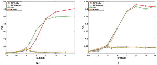
Figure 2.
Accuracy (PCL) as a function of the SNR, evaluated for 4 different models (the four markers and colors in the figure), on 2 different scenarios: (a) the gelmis mismatch; (b) the SWellEx-96 mismatch.
From the perspective of computational efficiency, the average execution time of the Bartlett algorithm is 0.01164 s, whereas that of the SBL algorithm is significantly longer at 7.4012 s in the case of limited computational resources. Additionally, it should be noted that considering predictable normal modes will further increase both computation and processing time. However, experimental results indicate that the proposed method effectively enhances localization accuracy for weak sources and mitigates issues related to localization misalignment or even complete failure due to environmental mismatches. The trade-off of a modest amount of computing time yields higher and more stable underwater weak source localization accuracy, making this approach feasible for practical ocean exploration applications. Therefore, it can be concluded from Figure 2 that the MPR-SBL algorithm has better localization accuracy than the SBL algorithm for weak sound sources in various scenarios, and can better locate and identify weak sound sources compared with MPR-Bartlett.
The RMSE of the weak source in range and depth is shown in Figure 3 and Figure 4, in which Figure 3a,b, respectively, represent RMSE in range and depth under the scenario of genlmis mismatch, and Figure 4a,b, respectively, represent RMSE in range and depth under the scenario of SWellEx-96 mismatch. Blue lines represent MFR-Bartlett results, red lines represent MPR-SBL results, yellow lines represent Bartlett results, and green lines represent SBL results. It can be seen from Figure 3 and Figure 4 that with the increase in SNR, RMSE decreases continuously and approaches a a constant value. The mean square error of SWellEx-96 in relation to water depth, sound velocity, and sediment properties is larger than that of the genlmis scene: the error in depth is close to 5 m and in range is close to 1 km in the genlmis scene, while the error in depth is close to 20 m and in range is close to 2 km in the SWellEx-96 scene. In the genlmis scene, MPR-SBL delivers results similar to SBL in terms of depth error, but the range error is smaller when the SNR is greater than 5 dB, which makes the PLC corresponding to MPR-SBL higher. In the SWellEx-96 scenario, MPR-SBL has slightly lower errors in depth and range than the SBL algorithm, which is consistent with its slightly higher PCL than SBL. In contrast, the RMSE of range for MPR-Bartlett and Bartlett processors is approximately 2 km, while the RMSE of depth exceeds 5 m in the genlmis mismatch scenario. In the SWellEx-96 mismatch scenario, the RMSE of range approaches 2.5 km, and the RMSE of depth is nearly 25 m. These findings illustrate the effectiveness and advancement of MPR-SBL in situations characterized by complete environmental mismatch. Furthermore, Figure 3 and Figure 4 basically verify the results in Figure 2.
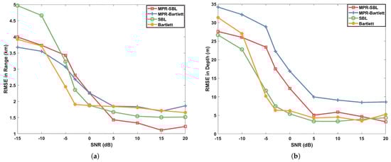
Figure 3.
Root mean square errors (RMSE) as a function of the SNR, evaluating the error variation trend of weak source in depth and range for 4 different models (the four markers and colors in the figure) under the scenario of a genlmis mismatch: (a) the range; (b) the depth.
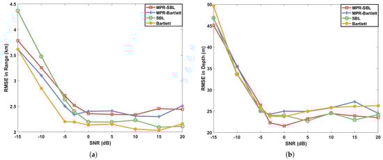
Figure 4.
Root mean square errors (RMSE) as a function of the SNR, evaluating the error variation trend of weak source in depth and range for 4 different models (the four markers and colors in the figure) under the scenario of a SWellEx-96 mismatch: (a) the range; (b) the depth.
3.4. The SWellEx-96 Experiments
In this section, the proposed MPR-SBL is tested on the SWellEx-96 Event S5 dataset, and compared with the Bartlett processor, MPR-Bartlett, and SBL.
The data recording time is 75 min in total, the sampling frequency is 1500 Hz, and the total number of sampling points equate to 6,750,000. The Caesar window with a length of 4096 and is used for spatial translation, and a overlapping Fast Fourier Transform (FFT) is used to transform the sampled data into the frequency domain. A total of 3294 groups of data are obtained. Considering Doppler shift, the FFT value with the largest absolute value in 2 FFT intervals near the specified frequency is selected. Two frequency signals, 166 Hz and 201 Hz, are selected for the experiment, because several algorithms have poor positioning results for the single frequency signal of this data.
The experimental environment configuration is similar to the SWellEx-96 scenario in Section 3.3. The experimental search range is from 0.05 km to 10 km, with an interval of 0.05 km, and a depth range of 10 m to 200 m with an interval of 10 m. We set the number of snapshots to . In order to check the estimation performance of the four algorithms for weak sound sources, two identical 3294 sets of data are superimposed in a staggered way in proportion, with an offset of 294 sets, thus ensuring that the distance between the two sound sources is close to 1 km. Therefore, when the snapshot number , the first to 142nd parts and the 14th to 156th parts of the original data are added to obtain the two-source scene. With dB, the power of the second sound source is times that of the first sound source. Considering the environmental mismatch and other issues, this paper selects the five largest peaks of the ambiguity surface for analysis.
In this section, all 75 min data are selected, totaling 142 groups. The specific experimental results are shown in Figure 5. The range and depth estimates of the MRP-Bartlett, MPR-SBL, SBL, and Bartlett, respectively, change with time. The red line indicates the recorded value of the Global Positioning System (GPS) on the ship, which is the theoretical value of the sound source range. When the time is before 50 min, the range error becomes larger because the sound source is farther away from the array. Due to the ship position recorded by GPS, the sound source dragged by the ship is affected by seawater and ship operation, which leads to the deviation between its position and the ship’s position, alongside problems such as environmental mismatch. The estimated values of the three algorithms deviate from the theoretical values because their trajectories are basically consistent with the ship’s operation, so the deviation is within an acceptable range. SBL and MPR-SBL produce better localization results than Bartlett and MPR-Bartlett, and the range error is smaller after 55 min. Compared with the other three methods, MPR-SBL is more obvious in locating weak sound sources, especially between 33 min and 43 min. Compared with MPR-Bartlett and Bartlett, MPR-SBL is better at locating weak sound sources, and the two Bartlett algorithms can hardly locate the second sound source. Compared with SBL, MPR-SBL improves the localization performance of weak sound sources, especially from 33 min to 43 min. The MPR-SBL algorithm can locate weak sound sources, but the SBL algorithm cannot locate weak sound sources. By analyzing the positioning results of a source with stronger power, it is evident that while all four processors can approximate motion trajectory, the trajectory obtained using MPR-SBL is significantly clearer. This indicates that MPR-SBL demonstrates superior positioning performance even in scenarios involving a single source. Therefore, the experiment demonstrates that the MPR-SBL algorithm outperforms the SBL algorithm in identifying and locating weak sound sources as well as single sources when there is a mismatch in the actual environment. In contrast, both the MPR-Bartlett and Bartlett algorithms struggle to effectively identify and locate weak sound sources.
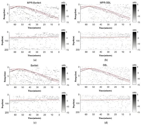
Figure 5.
Localization results of 4 different models on the SWellEx-96 dataset for two sources: (a) MPR-Bartlett; (b) MPR-SBL; (c) Bartlett; (d) SBL.
4. Conclusions
In this paper, we propose a MPR-SBL algorithm aimed at enhancing the accuracy and stability of underwater source localization, specifically addressing the environmental mismatch problem commonly encountered in traditional MFP. The algorithm integrates a predictable normal mode with sparse Bayesian learning (SBL), leveraging the sparse solution properties of SBL to improve the estimation of weak source locations. Compared to existing MFP algorithms and conventional SBL methods, our proposed algorithm demonstrates superior accuracy and stability in both range and depth estimations of the source.
Author Contributions
Conceptualization, B.Z., T.Z. and L.J.; methodology, R.J., L.J. and T.Z.; software, R.J.; validation, R.J., L.J. and L.Y.; formal analysis, B.Z., L.J. and T.Z.; investigation, R.J. and L.J.; resources, R.J. and L.J.; data curation, L.J.; writing—original draft preparation, B.Z. and L.Y.; writing—review and editing, B.Z. and L.Y.; visualization, R.J.; supervision, L.J. and T.Z.; project administration, L.J. All authors have read and agreed to the published version of the manuscript.
Funding
This research received no external funding.
Institutional Review Board Statement
Not applicable.
Informed Consent Statement
Not applicable.
Data Availability Statement
The data that support the findings of this study are available from the corresponding author.
Conflicts of Interest
The authors declare no conflicts of interest.
References
- Baggeroer, A.B.; Kuperman, W.A.; Mikhalevsky, P.N. An overview of matchedeld methods in ocean acoustics. IEEE J. Ocean. Eng. 1999, 18, 401–424. [Google Scholar] [CrossRef]
- Richardson, A.M.; Nolte, L.W. A posteriori probability source localization in an uncertain sound speed, deep ocean environment. J. Acoust. Soc. Am. 1991, 89, 2280–2284. [Google Scholar] [CrossRef]
- Dosso, S.E.; Wilmut, M.J. Uncertainty estimation in simultaneous Bayesian tracking and environmental inversion. J. Acoust. Soc. Am. 2008, 124, 82. [Google Scholar] [CrossRef] [PubMed]
- Schmidt, H.; Baggeroer, A.B.; Kuperman, W.A.; Scheer, E.K. Environmentally tolerant beamforming for high-resolution matched-field processing: Deterministic mismatch. J. Acoust. Soc. Am. 1990, 88, 1851–1862. [Google Scholar] [CrossRef]
- Krolik, J.L. Matched-field minimum variance beamforming in a random ocean channel. J. Acoust. Soc. Am. 1992, 92, 1408–1419. [Google Scholar] [CrossRef]
- Yang, T.C. A method of range and depth estimation by modal decomposition. J. Acoust. Soc. Am. 1998, 82, 1736–1745. [Google Scholar] [CrossRef]
- Bogart, C.W.; Yang, T.C. Comparative performance of matched mode and matched field localization in a range dependent environment. J. Acoust. Soc. Am. 1992, 92, 2051–2068. [Google Scholar] [CrossRef]
- Hinich, M.J.; Sullivan, E.J. Maximum-likelihood passive localization using model filtering. J. Acoust. Soc. Am. 1989, 85, 214–219. [Google Scholar] [CrossRef]
- Shang, E.C.; Clay, C.S.; Wang, Y.Y. Passive harmonic source ranging in waveguides by using mode fillter. J. Acoust. Soc. Am. 1985, 78, 172–175. [Google Scholar] [CrossRef]
- Wilson, G.R.; Koch, R.A.; Vidmar, P.J. Matched mode localization. J. Acoust. Soc. Am. 1988, 84, 310–320. [Google Scholar] [CrossRef]
- Porter, M.B. The KRAKEN Normal Mode Program. 1992. Available online: https://ui.adsabs.harvard.edu/abs/1992knmp.book.....P (accessed on 29 October 2024).
- Tabrikian, J.; Krolik, J.L.; Messer, H. Robust maximum-likelihood source localization in an uncertain shallow-water waveguide. J. Acoust. Soc. Am. 1996, 101, 241–249. [Google Scholar] [CrossRef]
- Gemba, K.L.; Nannuru, S.; Gerstoft, P.; Hodgkiss, W.S. Multi-frequency sparse bayesian learning for robust matched field processing. J. Acoust. Soc. Am. 2017, 141, 3411–3420. [Google Scholar] [CrossRef] [PubMed]
- Liu, Z.; Sun, C.; Yang, Y.; Du, J. Robust Source Localization Using Predictable Mode Subspace in Uncertain Shallow Ocean Environment; Oceans: San Diego, CA, USA, 2014; pp. 1–5. [Google Scholar]
- Vashishtha, G.; Kumar, R. An amended grey wolf optimization with mutation strategy to diagnose bucket defects in Pelton wheel. Measurement 2022, 187, 110272. [Google Scholar] [CrossRef]
- Vashishtha, G.; Kumar, R. An effective health indicator for the Pelton wheel using a Levy flight mutated genetic algorithm. Meas. Sci. Technol. 2021, 32, 094003. [Google Scholar] [CrossRef]
- Porter, M.; Tolstoy, A. The Matched-field processing benchmark problems. J. Comput. Acoust. 1994, 2, 161–185. [Google Scholar] [CrossRef]
- Gerstoft, P.; Mecklenbruker, C.F.; Xenaki, A.; Nannuru, S. Multisnapshot sparse bayesian learning for doa. IEEE Signal Process. Lett. 2016, 23, 1469–1473. [Google Scholar] [CrossRef]
- Gemba, K.L.; Hodgkiss, W.S.; Gerstoft, P. Adaptive and compressive matched field processing. J. Acoust. Soc. Am. 2017, 141, 92–103. [Google Scholar] [CrossRef] [PubMed]
Disclaimer/Publisher’s Note: The statements, opinions and data contained in all publications are solely those of the individual author(s) and contributor(s) and not of MDPI and/or the editor(s). MDPI and/or the editor(s) disclaim responsibility for any injury to people or property resulting from any ideas, methods, instructions or products referred to in the content. |
© 2024 by the authors. Licensee MDPI, Basel, Switzerland. This article is an open access article distributed under the terms and conditions of the Creative Commons Attribution (CC BY) license (https://creativecommons.org/licenses/by/4.0/).