Detection of Exoplanets in Transit Light Curves with Conditional Flow Matching and XGBoost

Abstract

NASA’s space-based telescopes Kepler and Transiting Exoplanet Survey Satellite (TESS) have detected billions of potential planetary signatures, typically classified with Convolutional Neural Networks (CNNs). In this study, we introduce a hybrid model that combines deep learning, dimensionality reduction, decision trees, and diffusion models to distinguish planetary transits from astrophysical false positives and instrumental artifacts. Our model consists of three main components: (i) feature extraction using the CNN VGG19, (ii) dimensionality reduction through t-Distributed Stochastic Neighbor Embedding (t-SNE), and (iii) classification using Conditional Flow Matching (CFM) and XGBoost. We evaluated the model on two Kepler and one TESS datasets, achieving F1-scores of 98% and 100%, respectively. Our results demonstrate the effectiveness of VGG19 in extracting discriminative patterns from data, t-SNE in projecting features in a lower dimensional space where they can be most effectively classified, and CFM with XGBoost in enabling robust classification with minimal computational cost. This study highlights that a hybrid approach leveraging deep learning and dimensionality reduction allows one to achieve state-of-the-art performance in exoplanet detection while maintaining a low computational cost. Future work will explore the use of adaptive dimensionality reduction methods and the application to data from upcoming missions like the ESA’s PLATO mission.

1. Introduction

Since the discovery of 51 Pegasi b [1], the identification of exoplanets—planets orbiting stars other than the Sun—has become one of the most rapidly evolving research fields combining a wide range of expertise from astrophysics to data science [2]. Over the past two decades, space-based telescopes such as NASA’s Kepler [3] and the Transiting Exoplanet Survey Satellite (TESS) [4] have revolutionized this field by collecting photometric measurements from hundreds of thousands of stars. By using the transit method [5], these telescopes have identified a large number of periodic signals due to real planets, astrophysical events (e.g., eclipsing binaries and stellar variability), and other phenomena (e.g., instrumental systematics). The human-based analysis is the most reliable approach to classify these signals as expert astronomers can handle a wide range of possible scenarios based on their expertise [6,7]. However, the manual examination of these signals presents two major drawbacks. First, human judgment is not objective, and some astronomers might disagree on labels assigned to some signals. Second, this process is highly time-consuming considering that astronomers need to be trained on this task [8] and that labeling a single signal might require from a few hours up to several days as the visual examination of Data Validation reports provided for the signal of interest [9] is required at least.

To address these issues, Convolutional Neural Networks (CNNs) [10] became the standard in classifying these signals [11,12,13,14,15], from their first implementation by Shallue C. and Vanderburg A. [16] (hereinafter SV18) with Astronet. These CNNs detect the most relevant patterns in transit signals through a feature extraction block—which is typically based on the architecture of the CNN VGG19 [17]—thus performing classification leveraging the universal approximation property of a Multi-Layer Perceptron (MLP) [18,19,20]. Over time, the architecture of these networks has been optimized, leading to significant performance gains up to 99% of classification accuracy on real exoplanet signals [21,22].

However, such CNNs are designed assuming that features useful for humans in their analysis are equally relevant to the model in solving the task at hand. Processing linearly dependent input features unnecessarily increase the complexity of the network [23], both in terms of data collection and preparation, and model’s parameter optimization. Moreover, the higher the number of model’s parameters requiring optimization, the larger the volume of training data needs to be in order for the optimization algorithm to converge to a stable local minimum; in this field, the ratio of the dataset size to the number of model parameters is still heavily skewed toward the latter. CNNs face two major limitations: their classifier is highly complex, consisting of hundreds of thousands to millions of parameters, and they lack interpretability, which is crucial here to understand the reasoning behind model predictions.

Decision trees such as Random Forests (RFs) [24] and Gradient Boosted Trees (GBTs) [25,26], including XGBoost, have demonstrated their effectiveness in approximating complex distributions with lower computational costs than MLPs. These models are universal approximators like MLPs [27] but obtain particularly better classification performance on tabular data [28]. Previous efforts demonstrated the effectiveness of RF classifiers in classifying planetary candidates across ground- and space-based surveys [29,30,31,32].

Another promising approach to preserve classification accuracy while reducing model complexity is dimensionality reduction (DR). Methods like t-Distributed Stochastic Neighbor Embedding (t-SNE) [33] can effectively project high-dimensional data into lower-dimensional embedding while preserving data structures, making them highly suitable for data processing before classification. Integrating the potential of these models can facilitate the development of a more efficient classifier. In this context, Armstrong D. et al. [30] and Schanche N. et al. [32] introduced innovative approaches, respectively, employing the combination of RFs and a Self-Organizing Map (SOM) for classifying transit signals in the Next-Generation Transit Survey (NGTS) [34] data and RFs coupled with a CNN for processing data from the Wide Angle Search for Planets (WASP) [35] survey.

In this paper, we propose an innovative approach to perform a multi-class classification of the signals detected in Kepler and TESS data, in planet candidate (PC), astrophysical false positive (AFP), and non-transiting phenomenon (NTP). Our approach is based on a model consisting of three main components:

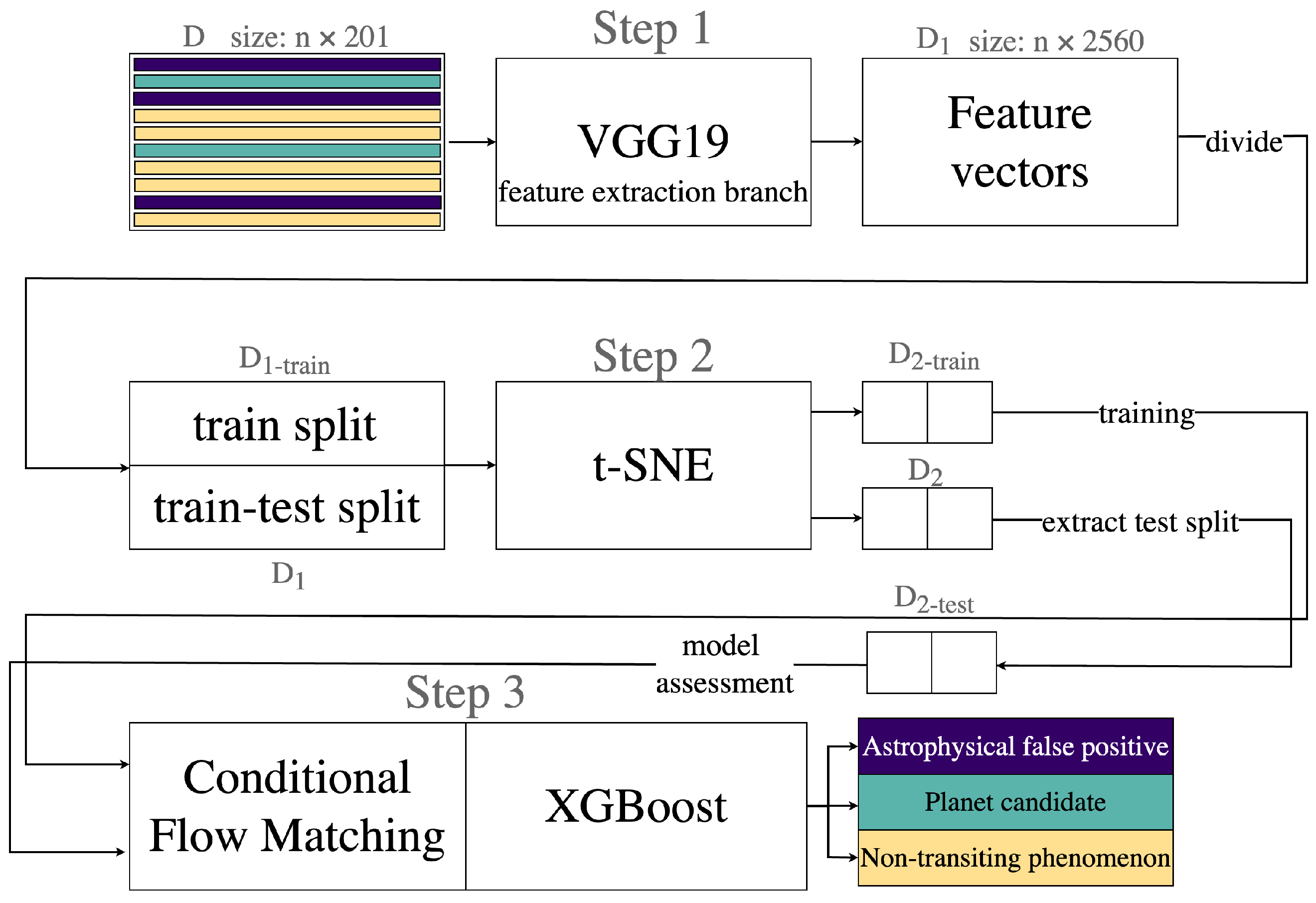
• Feature extraction, performed using the widely adopted CNN VGG19, which transforms input signals into high-dimensional feature vectors;
• Dimensionality reduction, performed by the t-SNE method, which maps the high-dimensional features to a lower dimensional space, where they can be most effectively classified;
• Classification, implemented by Conditional Flow Matching (CFM) and XGBoost [36].

Our model achieves competitive performance compared to the state of the art, with an F1-score of 99% on Kepler data and 100% on a TESS dataset, operating on very small inputs in size terms compared to other approaches in the literature.

Our results reveal that the application of t-SNE on the feature vectors produced by VGG19 enhances classification capabilities of the model than classical VGG-based CNNs classifying feature vectors with a MLP.

With this model, we continue to build on the most relevant architectures in the context of exoplanets detection (i.e., CNNs and decision trees), with the innovation of merging them in a single data processing pipeline. This work highlights the advantages of combining deep learning with dimensionality reduction and decision tree classifiers, offering an effective and efficient solution for exoplanet detection.

The rest of the paper is organized as follows: Related works are presented in Section 2, where we also define the contribution and novelty of our approach. The Kepler and TESS data used in this work are described in Section 3.1, while a theoretical background on the three main components of our model is provided in Section 3.2. We explain our model’s architectural details in Section 4, showing the results in Section 5. A discussion is reported in Section 6, including a comparison with related works, and conclusions are drawn in Section 7.

2. Related Works

This section provides an overview of the evolution of ML models for the classification of TCEs. Since numerous contributions have been made in this field, we summarize in Table 1 the specifics about the most relevant model architectures in order to highlight the key differences between prior studies and our approach.

The first ML models developed for the binary classification of TCEs were based on RFs, namely, Autovetter [29] and Robovetter [37]. These models were employed to classify thousands of Kepler TCEs and played a key role in generating two of the largest labeled datasets available for this survey: Kepler Q1–Q17 Data Release 24 and 25. Both approaches were designed to process a broad set of inputs, including scalar planetary features, centroid motion and difference image analysis, odd–even transit differences, secondary view, and phase-folded light curves (all these features are described in the caption of Table 1).

Subsequent efforts demonstrated that integrating different ML techniques lead to better classification performance. SOMs were applied to Kepler and K2 [38] data [39], while RF and SOM (RFC + SOM) combinations were tested on NGTS [30,34] data, and a model based on RF and CNN was applied on WASP data [32,35]. These hybrid approaches leveraged the strengths of different methods to improve robustness in TCE classification. These models used a limited set of input features, with SOM processing phase-folded light curves representing the transit shapes, while RFC + SOM integrates planetary parameters without centroid or secondary eclipse information. Although centroid information could help in identifying some false-positive scenarios such as background eclipsing binaries, in their work, Armstrong D. et al. [30] decided to not use this feature due to the risk to discard blended transiting planets, which instead remain candidates worthy of further analysis.

The introduction of deep learning revolutionized TCE classification, with CNN-based models becoming the standard. Astronet [16] was one of the first CNNs specifically designed for Kepler TCEs classification, processing a global view and its zoomed-in representation (the local view). Since then, CNN-based models have been used on various surveys, including K2 [11] and TESS [13,40]. Some models further increased input dimensionality by incorporating stellar and transit parameters alongside multiple light curves representations [14,41]. The evolution of CNNs culminated in two of the best models: Exominer [21] for Kepler and Astronet-Triage-v2 [22] for TESS. As shown in Table 1, both models process a combination of light curve representations (e.g., global and local views and secondary eclipse) and stellar and transit parameters to classify TCEs. Given that the input information processed by these models corresponds almost entirely to that used by astronomers during manual vetting, efforts to enhance their interpretability have become increasingly relevant. In this context, a notable contribution was proposed by Salinas H. et al. [42]. The authors of this study presented a Transformer-based approach for the binary classification of TESS TCEs, processing global and local views, centroid information, and stellar and planetary features.

Table 1. Comparison of different model architectures. For each model, we report the network architecture and the classification task (binary: 2c, or multi-class: >2c) and, if the model uses stellar features (St.f), planetary features (Pl.f, including transit period, transit duration, transit depth difference, etc.), centroid information (C, pixel-level information about the location of the variation in brightness for the detected transit), phase-folded flux (Pff, consisting of light curves with different data binning such as global and local views), odd–even (two consecutive transits), secondary view (Sv, consisting of the dip in star brightness when the detected object passes behind its star), difference image (Diff.img, used to evaluate whether the transit occurs out of the central pixel where the target star is supposed to be). The ✓ symbol indicates that the corresponding feature is used as an input parameter in the model; conversely, the symbol × indicates that the feature is not employed by the model.

Model [Ref.]	Architecture	Task	St.f.	Pl.f.	C	Pff	Odd–Even	Sv	Diff.img.
Robovetter	Decision Tree	3c	×	✓	✓	✓	✓	✓	✓
Autovetter	Decision Tree	3c	✓	✓	✓	✓	✓	✓	✓
Armstrong D. et al. [39]	SOM	2c	×	×	×	✓	×	×	×
Armstrong D. et al. [30]	RFC + SOM	2c	×	✓	×	×	×	×	×
Astronet	CNN	2c	×	×	×	✓	×	×	×
Astronet-K2 [11]	CNN	2c	✓	✓	×	✓	×	×	×
Exonet [41]	CNN	2c	✓	×	✓	✓	×	×	×
Genesis [43]	CNN	2c	✓	×	✓	✓	×	×	×
Astronet-Triage [13]	CNN	2c	×	×	×	✓	×	×	×
Astronet-Vetting [13]	CNN	2c	×	✓	×	✓	×	✓	×
Astronet-Triage-v2	CNN	5c	✓	✓	×	✓	×	✓	×
Exominer	CNN	2c	✓	✓	✓	✓	✓	✓	✓
Salinas H. et al. [42]	Transformer	2c	✓	✓	✓	✓	×	×	×
This work	CNN + DR + CFM + XGBoost	3c	×	×	×	✓	×	×	×

Table 1. Comparison of different model architectures. For each model, we report the network architecture and the classification task (binary: 2c, or multi-class: >2c) and, if the model uses stellar features (St.f), planetary features (Pl.f, including transit period, transit duration, transit depth difference, etc.), centroid information (C, pixel-level information about the location of the variation in brightness for the detected transit), phase-folded flux (Pff, consisting of light curves with different data binning such as global and local views), odd–even (two consecutive transits), secondary view (Sv, consisting of the dip in star brightness when the detected object passes behind its star), difference image (Diff.img, used to evaluate whether the transit occurs out of the central pixel where the target star is supposed to be). The ✓ symbol indicates that the corresponding feature is used as an input parameter in the model; conversely, the symbol × indicates that the feature is not employed by the model.

Model [Ref.]	Architecture	Task	St.f.	Pl.f.	C	Pff	Odd–Even	Sv	Diff.img.
Robovetter	Decision Tree	3c	×	✓	✓	✓	✓	✓	✓
Autovetter	Decision Tree	3c	✓	✓	✓	✓	✓	✓	✓
Armstrong D. et al. [39]	SOM	2c	×	×	×	✓	×	×	×
Armstrong D. et al. [30]	RFC + SOM	2c	×	✓	×	×	×	×	×
Astronet	CNN	2c	×	×	×	✓	×	×	×
Astronet-K2 [11]	CNN	2c	✓	✓	×	✓	×	×	×
Exonet [41]	CNN	2c	✓	×	✓	✓	×	×	×
Genesis [43]	CNN	2c	✓	×	✓	✓	×	×	×
Astronet-Triage [13]	CNN	2c	×	×	×	✓	×	×	×
Astronet-Vetting [13]	CNN	2c	×	✓	×	✓	×	✓	×
Astronet-Triage-v2	CNN	5c	✓	✓	×	✓	×	✓	×
Exominer	CNN	2c	✓	✓	✓	✓	✓	✓	✓
Salinas H. et al. [42]	Transformer	2c	✓	✓	✓	✓	×	×	×
This work	CNN + DR + CFM + XGBoost	3c	×	×	×	✓	×	×	×

Our approach integrates the key strengths of previous models into a unified framework. We adopt CNN architecture based on VGG19 as feature extractor, a choice consistent with previous works such as Astronet, Astronet-Triage, and Astronet-Triage-v2. However, instead of relying on the CNN for end-to-end classification as previous works already tested, we show that classification performance improves when features are projected into lower-dimensional spaces by t-SNE and that decision trees are used to exploit their capabilities in discriminating tabular data. We simplified the input to only the global view, deciding not to process as input the other light curves that differ from the global view in binning size (e.g., local view). Furthermore, the dimensionality reduction using t-SNE enhances computational efficiency and enables interpretability through the visualization of data in a two-dimensional space, providing insight into model predictions. A performance comparison with state-of-the-art models is provided in Section 6.4.

3. Background

Since our aim is developing a model to classify signals detected in transit light curves, this section is intended to provide all the necessary background information about the data used in this work (Section 3.1) and the operation of the methods that make up our model (Section 3.2).

3.1. Data

We work with light curves in which periodic transits of potential planetary nature, called Threshold-Crossing-Events (TCEs), were detected. Section 3.1.1 briefly explains how light curves are produced by the Kepler and TESS telescopes and how TCEs are detected. For a more detailed overview on this, we refer the reader to Jenkins J. et al. [44] and Jenkins J. et al. [45]. Section 3.1.2 provides details about the composition of TCEs datasets used. The process of input data preparation is described in Section 3.1.3.

3.1.1. From Light Curves to Threshold Crossing Events

The Kepler and TESS space telescopes were designed to gather photometric observations for a set of target stars from which light curves are extracted with a technique called aperture photometry. This technique consists of extracting the flux values of a target star from each photometric observation by summing the pixel values within a predefined aperture, optimized to maximize the signal-to-noise ratio (SNR). The resulting one-dimensional signal represents the variation in stellar brightness as a function of time, forming a light curve. An example of Kepler light curve is depicted in the top panel of Figure 1.

During its nine year service until 2018, Kepler monitored approximately 156,000 stars in a fixed region of the sky up to 4000 light years from the Earth, in the constellations of Lyra and Cygnus. The stellar flux measurements were sampled at 29.4 min cadence. Observations for each target star were divided into quarters of ∼90 days, after which the spacecraft rotated 90 degrees to maintain its solar panels pointed toward the Sun.

The observation strategy has changed with TESS, with the telescope scanning the entire sky in a 200-light-year range, dividing the sky into 26 sectors each observed for 27 days. TESS is designed to observe ∼200,000 target stars at a 2 min cadence (short cadence data) and to collect Full-Frame Images of each sector at 10 and 30 min cadences (long cadence data).

Both missions employ similar pipelines for data reduction and TCEs detection: the Kepler Science Operations Center (KSOC) [44] and the Science Processing Operations Center (SPOC) [45] for Kepler and TESS, respectively. These pipelines perform bias and flat field calibration, aperture photometry, and systematic corrections before identifying TCEs via the Transiting Planet Search module [46]. While SPOC is responsible for processing TESS short cadence data, long cadence data are processed by the MIT Quick Look Pipeline (QLP) [47].

3.1.2. Catalogs of Threshold Crossing Events Used in This Work

When TPS detects periodic dimming, i.e., TCEs, in the pre-processed stellar light curves, each TCE is examined by astronomers through automated tools [48] whose outputs are visually analyzed so that a label can be assigned to it [6,7]. This process, intent on determining the nature of each TCE, is called vetting.

In this study, we use three catalogs of labeled TCEs from which we produce the input representations we fed to our model. These catalogs provide for each TCE a set of physical (both planetary and stellar) and statistical parameters used for its classification and characterization. The parameters of these catalogs we used are those related to transit properties, i.e., transit period, duration, and the time of the first detected transit (defined as epoch), along with the column defining the label of the TCE. We employ these transit parameters during the pre-processing method, as described in Section 3.1.3.

• Kepler Q1–Q17 Data Release 24 (${\mathcal{D}}_{K24}$). This catalog comprises 20,367 TCEs identified by the KSOC pipeline in Kepler light curves. These TCEs were automatically classified by Autovetter [29,49] into planet candidates (PCs), astrophysical false positives (AFPs), non-transiting phenomena (NTP), and unknown (UNK). To minimize the uncertainty of our dataset labels, we adopted the approach employed for the first time by SV18 by discarding all TCEs labeled as UNK. This filtering resulted in a final dataset of 3600 PCs, 9596 AFPs, and 2541 NTPs.
• Kepler Q1–Q17 Data Release 25 (${\mathcal{D}}_{K25}$). This set is the final version of TCEs detected by the Kepler mission [50], comprising 34,032 TCEs automatically dispositioned by the Robovetter algorithm [37], that is an ensemble of decision trees trained on a dataset of labeled transits.
  The primary distinction between this catalog and ${\mathcal{D}}_{K24}$ lies in a higher number of long-period TCEs (approximately 372 days), resulting in ${\mathcal{D}}_{K25}$ being a TCE dataset characterized by a lower SNR. With longer orbital periods, the number of observed transits decreases, limiting the increase in SNR during our data preparation pipeline.
  Before generating model inputs from this catalog, we performed the following filtering operation. We removed all TCEs with the rogue flag set to 1, which correspond to cases with fewer than three detected transits, erroneously included in this catalog due to a bug in the Kepler pipeline. For our PC class, we selected the 2726 confirmed and 1382 candidate planets from the Cumulative KOI catalog (The Cumulative KOI catalog contains the most precise information on all the Kepler TCEs labeled as confirmed and candidate planet, as well as false positive. Further information about Kepler tables of TCEs can be found at the following link: https://exoplanetarchive.ipac.caltech.edu/docs/Kepler_KOI_docs.html, accessed on 9 August 2024). Our AFP class includes the 3946 TCEs labeled as false positive in the Cumulative KOI table, while the NTP class contains the 21,098 TCEs from the Kepler Data Release (DR) 25 catalog that do not appear in the Cumulative KOI table.
• TESS TEY23 (${\mathcal{D}}_{TEY23}$). This catalog contains a subset of 24,952 TCEs detected by QLP in TESS long cadence data for which Tey E. et al. [22] (hereafter TEY23) provided dispositions across a three-year vetting process. The authors used five labels to classify these TCEs: “periodic eclipsing signal”, “single transit”, “contact eclipsing binaries”, “junk”, and “not-sure” (see Section 2.4 of their paper for further details on the labeling process). To improve the reliability of our dataset, we filtered out (i) 5340 TCEs for which the authors did not provide a consensus label and (ii) all the TCEs labeled as “single transit” and “not-sure”, thus obtaining 2613 periodic eclipsing signals (we will identify as E), which include both planet candidates and non-contact eclipsing binaries, 738 contact eclipsing binaries (B) and 15,791 junk (J).

We divided each dataset in 80% training and 20% test splits. In dividing the dataset into the training test, we created splits by preserving the same percentage for each class as in the complete set. By doing so, we avoided getting unbalanced splits toward one of the classes.

Table 2. Composition of the three datasets used in this study. For each class *, we report the total number of TCEs and their distribution in training (80%) and test (20%) sets. * Classes. PC: Planet Candidate, AFP: Astrophysical False Positive, NTP: Non-Transiting Phenomenon, E: Periodic Eclipsing Signal, B: Contact Eclipsing Binary, and J: Junk. ^a The number of samples for the PC classes was doubled as described in Section 3.1.3.

Dataset [Ref.]	Class	Total	Training	Test
Kepler Q1–Q17 DR24 [49]	PC	a 7200	5760	1440
	AFP	9596	7676	1920
	NTP	2541	2033	508
	Total	19,337	15,469	3868
Kepler Q1–Q17 DR25 [50]	PC	a 8216	6573	1643
	AFP	3946	3162	784
	NTP	21,098	16,950	4148
	Total	33,260	26,685	6575
TESS TEY23 [22]	E	2613	1647	966
	B	738	598	140
	J	15,791	13,327	2464
	Total	19,142	15,572	3570

summarizes the composition of these datasets.

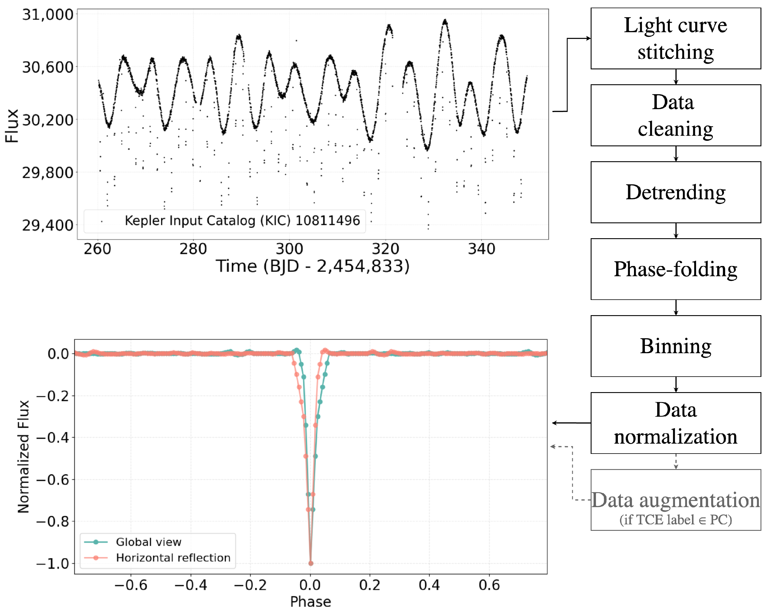
3.1.3. Data Preparation

The TCEs detected by the KSOC, SPOC, and QLP pipelines still remain signals dominated by the brightness of their host star, in our case, representing noise. To prevent our model from learning the noise, we generate a standard one-dimensional representation for each TCE: a binned and phase-folded light curve devoid of any variability except that of the transit of interest. The methodology we adopted to generate such representations has been widely used in this context of exoplanets detection with Machine Learning (ML) since it was proposed by SV18, and it is described below.

This data preparation pipeline consists of two main blocks: data cleaning—where inconsistent data such as not-a-number and outliers are removed—and data smoothing—where any variability in light curve brightness except that caused by TCE is flattened.

First, we download from the Mikulski Archive for Space Telescopes (MAST) (https://archive.stsci.edu/, accessed on 19 June 2020 for ${\mathcal{D}}_{K24}$, 20 May 2023 for ${\mathcal{D}}_{TEY23}$ and 9 August 2024 for ${\mathcal{D}}_{K25}$) the light curves of the stars around which the TCEs of the catalogs ${\mathcal{D}}_{K24}$, ${\mathcal{D}}_{K25}$, and ${\mathcal{D}}_{TEY23}$ orbit. For each TCE, we apply the following operations:

• Stitching the light curves. A TCE can be associated with multiple segments (Kepler quarters or TESS sectors) of the light curve of its host star. This depends mainly on the observing strategy of the telescope. We generate a single light curve by sequentially appending segments, which we then normalize by the median value calculated over the entire signal;
• Data cleaning. From the resulting light curve, we discard all not-a-numbers and outliers beyond $\pm 3\sigma$ of the stellar flux;
• Detrending. In order to remove any non-TCE-related variability, we divide the cleaned flux data by an interpolating polynomial of degree 3 computed using the Savitzky–Golay method with filter window set to 11. During detrending, we preserve flux measurements related to TCE transit by applying a mask calculated based on TCE transit period and duration;
• Phase-folding and binning. This detrended signal is folded on the relative TCE period and binned with a time bin size of 30 min (When developing this data pre-processing pipeline, we tested time bin sizes of 2, 10, and 30 min, which correspond to the data sampling rates of the Kepler and TESS telescopes. The best results in terms of the shape of the resulting transit were obtained using the 30 min value).
  Following the same methodology used by SV18 and Yu L. et al. [13], we linearly interpolate any empty bin so as to generate an input signal of length 201;
• Normalizing the binned signal. The binned signal is then normalized to 0-median and maximum transit depth to −1. We define the binned and normalized transit as global view, consisting of the one-dimensional input we fed to our model;
• Data augmentation on the PC class. Since our main goal is to train a model able to minimize the number of misclassified planets, we double the number of samples belonging to this class in the ${\mathcal{D}}_{K24}$ and ${\mathcal{D}}_{K25}$ datasets. More precisely, we apply a horizontal reflection to the global views of the PC TCEs. We decided to not adopt the same procedure to the eclipsing signals (E class) of ${\mathcal{D}}_{TEY23}$ since Tey E. et al. [22] declared that this set of planets also contains a fraction of non-contact eclipsing binaries, and we want to minimize the risk of increasing the number of eclipsing binaries contaminating the E class because of our purpose of identifying exoplanets.

The schema of this data preparation pipeline is depicted in Figure 1.

This pipeline is highly time-consuming because of (i) the large number of light curves to be processed (∼64,000); (ii) the multiple scans to be performed on each of them; (iii) the high number of data points for each light curves, up to 70,000. To speed up this process, we parallelized this pipeline by distributing the workload over multiple nodes as described in Fiscale S. et al. [51] as the operations on different light curves are independent.

3.2. Components of Our Model

Our model combines neural networks and other methods for feature extraction, dimensionality reduction, and the classification of global views. Below, we provide a theoretical background of each component of our model.

3.2.1. Convolutional Neural Network and VGG19

A Convolutional Neural Network [10,52] is a deep learning model consisting of two main blocks: (i) feature extraction—where the input is subjected to a series of operations such as application of convolutional filters, non-linear activation functions such as Rectified Linear Unit (ReLU), and spatial dimensionality reduction, i.e., pooling. The aim is to extract increasingly complex features from the data and identifying possible patterns, undetectable by manual examination, useful in solving the task at hand; (ii) classification—where the features extracted from the previous block are processed through a classifier, which is typically a MLP.

In this work, we exploited the feature extraction block of VGG19 to extract from our input data, the global views, and their most relevant features. The details of this process are described in Step 1 of Section 4.

3.2.2. Dimensionality Reduction and t-SNE

Dimensionality reduction methods aim to project high-dimensional data in a lower-dimensional space while preserving as much of the significant structure of the data as possible. Among the several dimensionality reduction algorithms (e.g., Isomap [53], Locally Linear Embedding [54], and Laplacian Eigenmaps [55]), we used t-SNE. It is a non-linear method that improves the Stochastic Neighbor Embedding algorithm [56] in terms of cost function optimization and solving the crowding problem (A comprehensive technical description of the t-SNE algorithm, including a quantitative analysis of how it preserves the local and global structure of high-dimensional data, can be found in the original paper by Van der Maaten L. and Hinton G. [33]. In particular, Sections 3.2 and 3.3 and Figures 1 and 2 of the aforementioned paper illustrate how the algorithm addresses the crowding problem and enhances cluster separation in the embedded space). t-SNE generates a two- or three-dimensional representation of input data as follows.

Let $\mathcal{X}={\left\{\overrightarrow{x_i}\right\}}_{i=1}^m\in {\mathbb{R}}^N$ the set of input data belonging to the N-dimensional space and $\mathcal{Y}={\left\{\overrightarrow{y_i}\right\}}_{i=1}^m\in {\mathbb{R}}^d$ the counterpart set of projections into the output lower-dimensional space, where $d\in \{2,3\}:d\le N$. In the input space, the pairwise similarities are modeled as conditional probabilities $p_{j|i}$, with

$$p_{j|i}={\displaystyle \frac{exp(-||{\overrightarrow{x}}_i-{\overrightarrow{x}}_j|{|}^2/2{\sigma }_i^2)}{{\sum }_{k\ne i}exp(-||{\overrightarrow{x}}_i-{\overrightarrow{x}}_k{\left|\right|}^2/2{\sigma }_i^2\left)\right)}}$$

(1)

where ${\sigma }_i$ is the variance of the gaussian distribution centered in the i-th sample. These conditional probabilities are symmetric since $p_{ij}=(p_{j|i}+p_{i|j})/2m$.

In the output space, similarities are modeled by using the t-Student distribution with one degree of freedom:

$$q_{ij}={\displaystyle \frac{(1+||{\overrightarrow{y}}_i-{\overrightarrow{y}}_j{\left)\right||}^2{)}^{-1}}{{\sum }_{k\ne l}(1+||{\overrightarrow{y}}_k-{\overrightarrow{y}}_l{\left)\right||}^2{)}^{-1}}}$$

(2)

The aim is to determine the points ${\overrightarrow{y}}_i$ so that the Kullback–Leibler (KL) divergence [57] between the two conditional probabilities distributions is minimized:

$$\mathrm{KL}\left(P\right|\left|Q\right)=\sum _{i\ne j}{p}_{ij}log{\displaystyle \frac{p_{ij}}{q_{ij}}}$$

(3)

The minimization of the quantity KL($P\left|\right|Q$) is computed with the gradient descent algorithm with momentum and adaptive learning rate (see Equation (5) in Van der Maaten L. and Hinton G. [33]). The momentum term increases during the gradient descent iterations, while the learning rate is updated according the method provided by Jacobs R.A. [58]. A full derivation of the t-SNE gradient can be found in Appendix A of the original paper. As the authors described in their Section 3.4, the optimization process is improved by the use of the “early exaggeration” trick, which forces the method to model large distances among the low dimensional representation of the samples based on their membership cluster. In other words, the distance between two samples of different clusters is maximized, as we found in our experiments and show in Figure 2.

We relied on t-SNE to reduce the dimensionality of feature vectors obtained from VGG19. Step 2 of Section 4 reports the details of this operation. We demonstrate in Section 5 that this dimensionality reduction places the data in a space where the classifier is able to define better separation surfaces that are highly discriminative than those learned from state-of-the-art CNNs, which work in higher dimensionality embeddings. The limitations of this technique are discussed in Section 6.5.

3.2.3. Gradient-Boosted Trees and XGBoost

Gradient-boosted trees (GBTs) consist of a set of sequentially trained decision trees highly robust in the classification of tabular data [59,60,61,62]. Each new tree is constructed with the aim of correcting errors made by previous trees. In a classification context, the final prediction on a given sample is obtained by the majority vote from the predictions of all the trees. In this study, we used eXtreme Gradient Boosting (XGBoost) [63], which differs from GBTs as the trees are constructed in parallel, rather than sequentially. In addition, XGBoost extends traditional gradient boosting by including regularization elements in the objective function, thus improving generalization and preventing overfitting issues, which is very important in exoplanet detection as the majority of datasets are highly imbalanced toward the not-PC classes.

3.2.4. Diffusion Models and Conditional Flow Matching

Diffusion models are the new frontier of generative models, long characterized by the domain of Generative Adversarial Networks [64]. Diffusion models iteratively transform input samples with the injection of noise and then learn to reverse this process, reconstructing the original samples distribution, by solving a Stochastic Differential Equation.

Conditional Flow Matching [36] is a diffusion model used in both generative and classification tasks [65]. CFM transforms an input sample through a learned vector field varying in time $t\in [0,1]$, mapping its original distribution to a Gaussian distribution over $n_t$ steps. This mapping is achieved by applying a series of invertible transformations (e.g., affine and planar transformations) on the sample, constrained by the labels of input data in supervised learning scenarios. At step $n_t$, the sample follows the reverse process by solving an Ordinary Differential Equation (ODE) so that the original data distribution can be reconstructed.

XGBoost plays a dual role in this framework. During the forward process, a new XGBoost model is trained at each step to estimate the vector field, providing a more efficient alternative than using a classical neural network [36,66]. Additionally, a final XGBoost is applied on the reconstructed sample at the end of the reverse process to perform classification.

We implemented CFM and XGBoost within our model by exploiting the approach provided by Jolicoeur-Martineau A. et al. [36].

4. Method

This section details the pipeline that we designed for the classification of global views, starting with feature extraction through a CNN, followed by dimensionality reduction via t-SNE, and concluding with classification using Conditional Flow Matching and XGBoost. We leverage the strengths of each component in our pipeline to achieve robust generalization performance in lower-dimensional spaces.

Let

$$\mathcal{D}=\{({\overrightarrow{x}}_1,y_1),({\overrightarrow{x}}_2,y_2),\dots ,({\overrightarrow{x}}_n,y_n)\}$$

be the input dataset composed by n samples. Each sample ${\left\{{\overrightarrow{x}}_i\right\}}_{i=1}^n\in {\mathbb{R}}^N$ consists of a global view of size $N=201$, with

$${\left\{y_i\right\}}_{i=1}^n\in \mathcal{Y}=\{\mathrm{AFP},\mathrm{PC},\mathrm{NTP},\mathrm{E},\mathrm{B},\mathrm{J}\}$$

indicating its label. The datasets ${\mathcal{D}}_{K24},{\mathcal{D}}_{K25}$, and ${\mathcal{D}}_{TEY23}$ are separately processed through the following steps.

• Feature extraction. We extract the features from the global views with the feature extraction block of VGG19. This model is independently trained on each dataset until overfitting on the global views. Since VGG19 is exclusively used as feature extractor, its training can be extended until overfitting the dataset in order to guarantee the most representative features are extracted. For each of the n global views, the VGG19’s feature extraction branch produces a one-dimensional feature map of size 2560, once flattened. We trained VGG19 for 300 epochs on each dataset, with a learning rate of $1\times {10}^{-3}$, batch size of 128, and pooling size and stride fixed to 3 and 2, respectively, by using Adam [67] as the optimization algorithm. As highlighted from the number of TCEs for each class in Table 2, all our datasets are imbalanced toward one of the three classes. Typically, such an imbalance is toward the class of non-astrophysical transits (classes NTP and J). To address class imbalance, we used class weighting when training VGG19. The weights for each class were computed using the Inverse Class Frequency technique [68].
  The n 2560-length feature vectors, we denote as ${\mathcal{D}}_1^{n\times 2560}$, are saved at the end of the last training epoch.
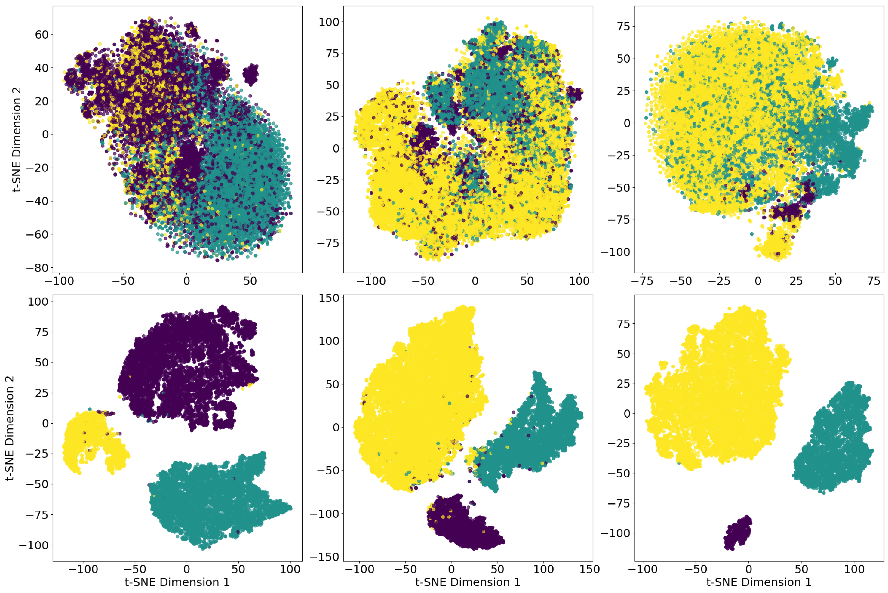
• Dimensionality reduction. The resulting feature vectors are projected into a two-dimensional embedding defined by t-SNE. By processing ${\mathcal{D}}_1$, t-SNE produces (In our experiments, we also evaluated the classification performance of our model by processing three-dimensional data produced by t-SNE, rather than exclusively two-dimensional data. However, the best performance was obtained by processing data in two dimensions) a representation ${\mathcal{D}}_2^{n\times 2}$.
  As shown in Step 2 of Figure 3, the input ${\mathcal{D}}_1$ of t-SNE is divided in two subsets (We discuss the application of this strategy in Section 6.5):
  • ${\mathcal{D}}_{1-train}$ (80% of data), used to generate ${\mathcal{D}}_{2-train}$, which will be used as training set for the Conditional Flow Matching;
  • The entire dataset ${\mathcal{D}}_1$, from which ${\mathcal{D}}_2$ is obtained. We extract from this representation the set ${\mathcal{D}}_{2-test}$, containing the data that will be used when assessing the Conditional Flow Matching performance.
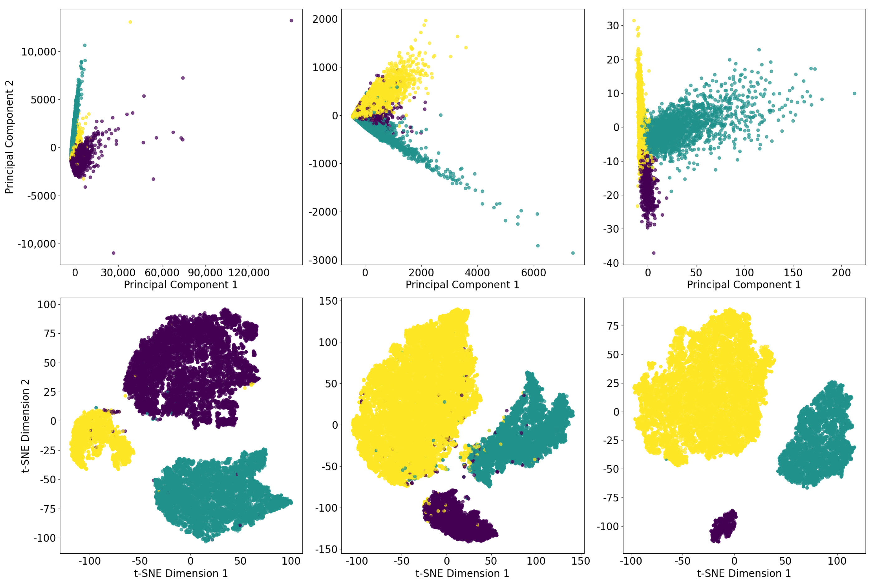
  Our experiments revealed that running t-SNE for 3000 iterations, with a perplexity of 50, best maximized the separation of TCEs classes in the two-dimensional space.
  The two-dimensional projections obtained by t-SNE for training and test data are shown in middle and right panels of Figure 2, respectively.
  We emphasize that a quantitative assessment of how well t-SNE preserves the clustering structure of the data—particularly in terms of local and global neighborhood relationships—is thoroughly discussed in the original work by Van der Maaten L. and Hinton G. [33]. In our study, we focus on the practical impact this dimensionality reduction has in the context of TCE classification, showing the related evidence in Figure 2 and Figure 4 and

  Table 3. Performance of different vetting models. Our precision, recall, and F1-scores for Kepler data are computed by averaging the scores of Table 4 obtained on each class. Other model scores are taken from the reference manuscripts. The best results on Kepler and TESS datasets are highlighted in boldface.

  Model [Ref.]	Survey	Precision	Recall	F1-Score
  SOM [39]	Kepler	0.864	0.865	0.864
  SOM [39]	K2	0.945	0.972	0.958
  RFC + SOM [30]	NGTS	0.901	0.914	0.907
  Exominer [21]	Kepler	0.968	0.974	0.971
  Exominer-Basic [21]	TESS	0.88	0.73	0.79
  Astronet-Triage-v2 [22]	TESS	0.84	0.99	0.909
  Transformer [42]	TESS	0.809	0.8	0.805
  This work	Kepler	0.974	0.987	0.980
  This work	TESS	1.0	1.0	1.0

  .
• Classification with CFM and XGBoost. Following the methodology described in Jolicoeur-Martineau A. et al. [36] and Li A. et al. [65], we performed TCE classification by processing ${\mathcal{D}}_2$ with CFM and XGBoost (Step 3). Each sample of ${\mathcal{D}}_2$ is mapped into the vector field of the CFM from $t=0$ to $t=1$ in $n_t=50$ steps. At each step, an XGBoost is trained to estimate the vector field. The sample at time $t=1$ is processed with an ODE, returning the output sample that is fed to an additional XGBoost, responsible for the TCE classification [65].
  Due to the low dimensionality of the input and the good separability between classes of TCEs provided by t-SNE, a very accurate classification performance is obtained as early as $n_t$ = 50 noise levels. Each of the $n_t$ XGBoosts has 100 decision trees of maximum depth of 2 and has been trained for 30 epochs with 63 steps per epoch. An extended discussion on finding the sub-optimal hyperparameters configuration is provided in Section 6.

5. Results

The results obtained from the model on the three datasets under this study are presented in this section. On each dataset, we evaluated the classification performance in terms of precision, recall, F1-score, and misclassification rate for each class [69].

Table 4. Classification performance of the model across three datasets: Kepler Q1–Q17 Data Release (DR) 24, Data Release 25, and TESS TEY23. The metrics, computed on test samples, show the ability of our model in distinguishing between TCEs of different natures, including Astrophysical False Positives (AFP), Planet Candidates (PC), and Non-Transiting Phenomena (NTP) in the Kepler datasets. For the TESS dataset, the classification involves TCEs whose nature could be non-contact eclipsing binaries (B), eclipsing signals (E), and Junk (J). For Kepler DR24, individual class misclassification rates are provided, showing particularly strong performance in identifying planet candidates (0.42% misclassification rate). On Kepler DR25, our model exhibits a global misclassification rate of 2.1% across all classes, while on TESS TEY23, it achieves robust predictions performance, with a 0% misclassification rate.

Dataset	Class	Precision	Recall	F1-Score	Misclass. Rate (%)
Kepler Q1–Q17 DR24	AFP	0.9943	0.9932	0.9937	1.25
	PC	0.9972	0.9986	0.9979	0.42
	NTP	0.9803	0.9803	0.9803	3.93
Kepler Q1–Q17 DR25	AFP	0.910	0.985	0.946	2.1
	PC	0.971	0.996	0.983
	NTP	0.997	0.972	0.984
TESS TEY23	B	1.000	1.000	1.000	0.0
	E	1.000	1.000	1.000
	J	1.000	1.000	1.000

reports these results. In general, the discriminatory capabilities of the model on each dataset are competitive with those obtained from state-of-the-art models [21,22].

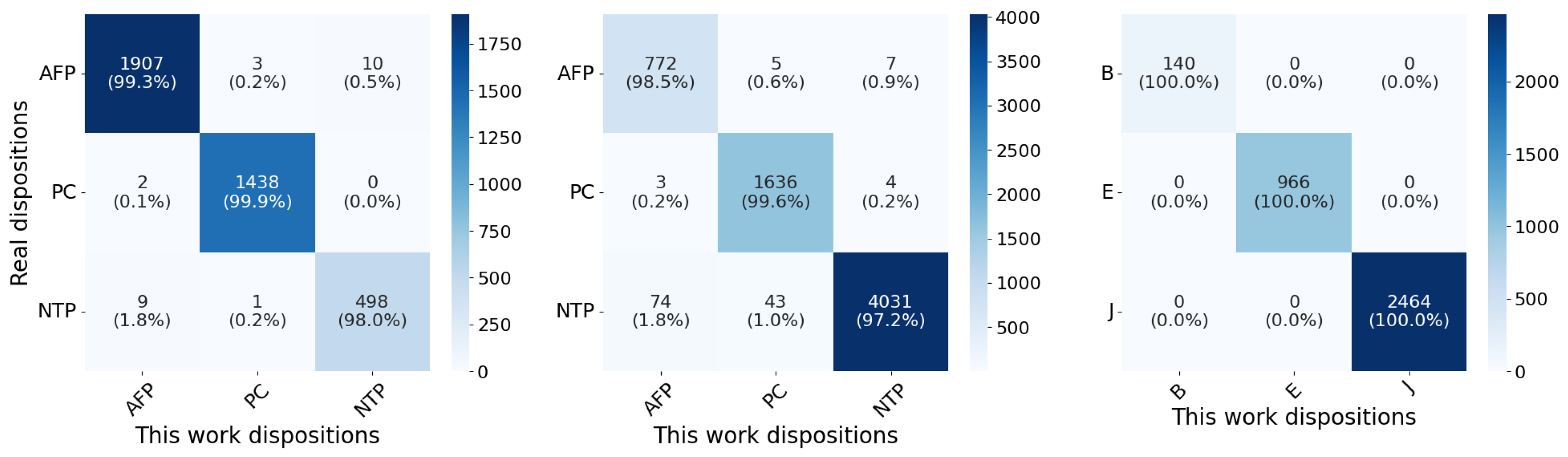
5.1. Application on Kepler Q1–Q17 Data Release 24

The model achieves high predictive accuracy across all three classes of ${\mathcal{D}}_{K24}$, with noteworthy results in the identification of planets. The results are reported in the first block of Table 4 and discussed below.

On the PC class, we obtain a precision of 0.9972, a recall of 0.9986, and an F1-score of 0.9979, with a misclassification rate of 0.042, indicating a very robust distinction between planetary signals and false positives or non-transiting phenomena. On the AFP class, the precision is 0.9943, recall 0.9932, and F1-score is 0.9937, resulting in a misclassification rate of 0.0125. The NTP class, while more challenging due to its variability in the nature of transits (including any transit not consistent with astrophysical ones), maintains optimal classification metrics, with a precision, recall, and F1-score of 0.9803 and a misclassification rate of 0.0393.

Analyzing the confusion matrix in left panel of Figure 5, we observe 25 TCE misclassified. The majority of these misclassifications occur between the AFP and NTP classes, counting 19 samples. These samples correspond to the purple and yellow points in the top right panel of Figure 2, which are located in regions of the two-dimensional space close to the center of a cluster to which they do not belong. For the PC class, our model misclassifies only two planets, labeling them as AFP. Meanwhile, there are only three false positives: two AFPs and one NTP, which are the purple and yellow points in the green cluster of the top right panel in Figure 2.

These results demonstrate the effectiveness of our model in distinguishing the TCEs of the three classes, particularly in the identification of planet candidates.

5.2. Application on Kepler Q1–Q17 Data Release 25

Compared to the DR24 dataset, the higher number of long-period TCEs with a lower SNR in ${\mathcal{D}}_{K25}$ slightly affects the classification accuracy of our model. Nevertheless, discrete classification performance is achieved on this dataset as well. The second block of Table 4 displays the results we present below.

For the AFP class, the model achieves a precision of 0.910, a recall of 0.985, and an F1-score of 0.946. For the PC class, very high scores are obtained: precision is 0.971, recall is 0.996, and F1-score is 0.983. For the NTP class, the model exhibits the highest precision of 0.997, along with a recall of 0.972 and an F1-score of 0.984.

The middle panel confusion matrix in Figure 5 shows that the number of misclassified planets is very low. The model successfully identifies 1636 planets out of 1643 total samples, with only seven misclassifications. Three are associated with the AFP class and four to the NTP class. Regarding these four TCEs, we focus the reader’s attention on the middle right panel of Figure 2. Among the five planets (green points) projected by t-SNE near regions dominated by NTPs, only four are classified as NTP. Our model is able to retrieve one of them during classification, despite the fact that its position in the two-dimensional space seemed to compromise its classification. The number of false positives is relatively high (48, including 43 NTPs and 5 AFPs). These samples are visible in middle right panel of Figure 2. The presence of a small cluster of yellow points and five purple points falling into the green cluster of the PCs can be observed. For these points, the model is unable to provide the correct label.

Overall, the misclassification rate of 0.021 further confirms the robust discrimination capabilities of the model on all three classes of TCEs, despite their imperfect separation in the two-dimensional space.

The results obtained on the two Kepler datasets show that the greatest uncertainty in the model lies in the discrimination between AFP and NTP class samples. However, the percentage of misclassifications between these two classes is extremely low (∼2%) and involves samples located at the edges of the clusters (as shown in the rightmost panels of Figure 2), suggesting that further analysis on these cases would not make significant contributions to the overall evaluation of the model. We recall that the main goal is to minimize the fraction of misclassified PCs as they represent the signals of greatest scientific interest. In this regard, our model performs very well: the maximum percentage of misclassified planets is 0.4% in ${\mathcal{D}}_{K25}$, a value that is very small. As mentioned in Section 3.1.2, ${\mathcal{D}}_{K25}$ is known to contain a higher fraction of long-period planets than ${\mathcal{D}}_{K24}$, resulting in fewer available transits and, consequently, a lower SNR of TCEs. This aspect may justify a slight increase in the misclassifications from ${\mathcal{D}}_{K24}$ (0.1%) to ${\mathcal{D}}_{K25}$ (0.4%). In Section 6.6, we discuss instead the problem of label noise, whereby a TCE of a given class (e.g., AFP) may change its disposition over time or be labeled differently by different teams of astronomers.

5.3. Application on TESS TEY23

As highlighted in third block of Table 4, our model shows impressive performance in classifying non-contact eclipsing binaries, eclipsing signals, and junk. The model correctly classifies all samples with no misclassified TCEs. As a result, precision, recall, and F1-score all reach their maximum value of 1, with a misclassification rate of 0%. The confusion matrix on this dataset is shown in right panel of Figure 5. The correct classification of all samples is mainly due to their perfect separation in two-dimensional space, as visible in the bottom right panel of Figure 2.

The results on the TESS dataset demonstrate that the prediction of our model is consistent with the labels assigned by experts, which we considered as ground truth. For the two Kepler datasets, our predictions align with the automated labels produced by Autovetter and Robovetter. These findings suggest that the proposed method exhibits strong robustness when applied to real data.

6. Discussion

6.1. The Contribution of VGG19 and t-SNE in TCEs Classification

The use of VGG19 for extracting features from the global views proved to be crucial in ensuring a highly discriminative representation of TCEs.

Initially, we evaluated the use of the CNN provided by Fiscale S. et al. [15] as a feature extractor that we will call DART-Vetter. This model, developed to classify Kepler and TESS TCEs, processes the global view through five convolutional blocks. Each block consists of a one-dimensional convolutional layer followed by ReLU activation, spatial dropout, max pooling, and batch normalization. The number of filters in the convolutional layers increases exponentially from 16 to 256. The extracted features are then flattened and classified through a single fully connected layer. Feature extraction from the global views of the three datasets was performed following the same procedure described in Section 4 (Steps 1 and 2). DART-Vetter was trained until overfitting on each dataset, and the extracted features were stored at the final training epoch.

However, the classification performance on feature vectors produced by DART-Vetter was poor. For this reason, we evaluated the use of VGG19. This network has already been widely used in the context of exoplanet identification, demonstrating its effectiveness since the introduction of Astronet, whose network architecture is clearly based on that of VGG19, as shown in Figure 7 of their paper [16].

Figure 4 presents a visual comparison of the features obtained from DART-Vetter (top panel) and VGG19 (bottom panel) for the ${\mathcal{D}}_{K24}$ (left panel), ${\mathcal{D}}_{K25}$ (middle panel), and ${\mathcal{D}}_{TEY23}$ (right panel) datasets. The results indicate that VGG19 provides a significantly more effective class separation, with minimal overlap between different classes, unlike the features extracted by DART-Vetter, where class overlap is more noticeable.

The left column of Figure 2 shows, for each dataset, the two-dimensional representations of global views before features are extracted from them using VGG19. Middle and right columns depict the two-dimensional representation—defined by t-SNE—of the features extracted from this network on the training and test data, respectively. The clear class separation achieved after feature extraction and dimensionality reduction confirms that VGG19 captures robust discriminative features, while t-SNE further enhances their separability, as highlighted by the results of Table 3. This near perfect separability facilitated the training of Conditional Flow Matching and XGBoost, enabling them to learn well-defined decision surfaces resulting in a very low misclassification rate.

Thus, the high classification accuracy of our model is mainly due to the key role of combining feature extraction and dimensionality reduction for the identification of most relevant patterns within the global views.

6.2. Reducing the High Computational Complexity and Memory Demand When Training the Conditional Flow Matching with XGBoost

In this section, we discuss a key factor we had to handle during the design of the model and which directed us toward the use of dimensionality reduction methods.

Training our CFM with XGBoost on the feature vectors extracted from VGG19 would have required an extremely high computational cost, making the whole process shown in Figure 3 impractical. We trained CFM and XGBoost with the methodology provided by Jolicoeur-Martineau A. et al. [36], which requires training $n_t$ models, where the levels of noise $n_t$ should take values in [50, 100]. In addition, each model needs to be trained on a duplication of the input dataset. For example, on Kepler Q1–Q17 Data Release 25, it would have been necessary to replicate the dataset at least 50 times, bringing the overall size to more than 1.6 million samples, each with 2560 features. This would have required significantly more memory resources than were available on our machine and training times on the order of several days, also hampering the hyperparameters fine-tuning. An even more critical issue concerned the scalability of the model: even if we had obtained good results, such an onerous process would have made it difficult for other users to exploit the model on their own laptops. The application of t-SNE proved its effectiveness also in addressing this issue by compressing the input vectors from 2560 to only 2 features.

This compression allowed us to preserve the discriminative patterns learned from VGG19 on the global views while ensuring efficient training of CFM with XGBoost and easily reproducible model configuration on common hardware.

To further assess the ability of t-SNE in mapping the feature vectors into a two-dimensional space, we made a comparison with Principal Component Analysis (PCA). As illustrated in Figure 6, t-SNE outperforms PCA in preserving class separability within the lower dimensional embedding. Left and central panels of Figure 6 (top row) demonstrate that when features from the ${\mathcal{D}}_{K24}$ and ${\mathcal{D}}_{K25}$ datasets are projected using PCA, they are partially overlapped and spread across significantly larger regions, resulting in poor cluster definition. For each dataset, the standard deviations (${\sigma }_1,{\sigma }_2$) of the first two principal components are ${\mathcal{D}}_{K24}$: (2903.8, 1551.8); ${\mathcal{D}}_{K25}$: (407.0, 224.2); ${\mathcal{D}}_{TEY23}$: (18.0, 5.8).

This wider spreading occurs because data with PCA are linearly mapped to the directions with largest variance, causing high variance classes to distribute across larger regions.

On the other hand, t-SNE maps the same features into more compact embedding while effectively preserving the separation between the three TCE classes. The better ability of t-SNE to project TCEs features into well-defined regions corresponding to their respective classes justifies our choice to adopt this method for dimensionality reduction in our pipeline.

6.3. Finding the Hyperparameter Configuration Optimizing Classification Accuracy

During the experiments, we conducted a systematic analysis of classification performance by varying the Conditional Flow Matching and XGBoost hyperparameters. As suggested in Jolicoeur-Martineau A. et al. [36], we tested noise levels in the range [50, 100], with discrete increments of 10 units. The optimal number of decision trees was evaluated by considering sets in [100, 500], each time increasing by 100 units. Given the two-dimensional inputs of our Step 3, an extensive exploration of the maximum depth of the trees was not necessary, limiting the analysis to architectures with depths of no more than four levels. The number of training epochs of decision trees was estimated in [10, 100], with increments of 10. The batch size for each epoch was chosen by preferring powers of 2 in order to optimize computational efficiency and maximize the use of available hardware resources. The value of 63 steps for each epoch allowed us to process batch sizes of similar size to 256. The experiments conducted revealed that the performance does not improve as model complexity increases. This result finds a natural interpretation in Occam’s razor heuristic, according to which, given equal performance, simpler models are preferable to their more complex counterparts.

6.4. Comparison with State-of-the-Art Vetting Models

In this section, we compare the predictive performance of our model with those achieved by state-of-the-art vetting models.

Table 5. Technical details regarding the deep learning models we compare for classification performance in Table 3. For each model, we provide information about the architecture and training hyperparameters. Input branches indicate the number of input channels through which the model processes data. The column Figure Ref. refers to the figure in the original article where the network architecture is shown. We derived the information displayed in this table from reference articles (and from related source codes when available). We were not able to retrieve the related information for the element denoted with the “-” symbol.

Hyperparameters	Models
	Exominer	Astronet-Triage-v2	Salinas H. et al. [42]
Architecture	CNN	CNN	Transformer
Figure Ref.	Figure 9	Figure 8	Figure 2
Input branches	8	7	3
Activation	ReLU	ReLU	Attention Mechanism *
Regularization	Dropout	Dropout	Dropout
Fully-connected	4 × 128	4 × 512	Linear (X → 2) *
Output	Sigmoid	Sigmoid	Softmax *
Optimizer	Adam	Adam	Adam
Training	-	20,000 steps	60 epochs
Learning rate	6.73 $\times {10}^{-5}$	1 $\times {10}^{-3}$	1 $\times {10}^{-3}$
Batch size	-	64	100
Model selection	10-fold CV	10-fold CV	10-fold CV
	Armstrong D. et al. [39]		Armstrong D. et al. [30]
	Kepler	K2
Architecture	SOM	SOM	RFC + SOM
Grid dimension	20 × 20	8 × 8	20 × 20
Radius	20	<20	20
Training epochs	500	500	300
Learning rate	0.1	0.1	0.1

* Softmax in the final layer, Attention Mechanism within the Transformer blocks. X represents the concatenated output dimension of the encoders.

reports the technical details regarding the models we compare with, while Table 3 summarizes the performance of these comparison models. Direct comparisons should be made with caution as these models are trained and tested on datasets from different surveys, varying in training and test set size and pre-processing methods. Additionally, each model applies a specific classification threshold, which is typically optimized on recall to minimize the fraction of misclassified planets.

Exominer achieves a precision of 0.96 and recall of 0.97, while Astronet-Triage-v2 attains 0.84 and 0.99, respectively. Despite their ability to minimize the fraction of false negatives, these models were designed to process human-relevant input features, some of which are linearly dependent. For example, the local view is essentially a global view with a different bin size. Including such redundant features increases model complexity without significantly improving generalization capabilities [23,43,70]. In addition, high-dimensional inputs increase the risk that the network will need substantial architectural changes to be applied to data from different surveys. This limitation is evident in the degraded performance of Exominer when applied to TESS data (Exominer-Basic), where its precision and recall drop to 0.88 and 0.73, respectively. While reducing input redundancy is crucial for optimizing model effectiveness, astronomers often prioritize interpretability to understand the reasoning behind model predictions. Salinas H. et al. [42] introduced a Transformer-based approach designed to enhance interpretability. However, its performance remains below that of Exominer and Astronet-Triage-v2, achieving a precision of 0.809 and recall of 0.8.

The SOM-based model proposed by Armstrong D. et al. [39] proves its robustness on K2 data, with an F1-score = 0.958, but the performance deterioratea on the Kepler dataset, where the F1-score is 0.864.

Compared to all previous approaches, our model achieves the highest scores on both Kepler and TESS datasets, with an F1-score of 0.980 and 1.0, respectively. Notably, this performance is achieved without increasing input dimensionality, consequently making our model easily transferable across surveys. Our implementation choices supported by promising results suggest that projecting the learned features into lower dimensional spaces and then classifying them by exploiting the capabilities of decision trees as universal approximators may be sufficient to outperform more complex models.

6.5. Current Limitations of Our Model

The current limitation of our approach is the use of t-SNE for dimensionality reduction. Unlike deep learning models, t-SNE lacks optimizable parameters and, therefore, cannot learn dynamic mappings from high- to low-dimensional space through a training phase. Consequently, to guarantee that the two-dimensional projection of training data is not influenced by test data during dimensionality reduction (as described in Step 2 of Section 4), we had to split ${\mathcal{D}}_1$ into distinct subsets.

Additionally, t-SNE is computationally expensive on large datasets as it requires computing pairwise distances. Although this method presents these drawbacks, it proved to be effective in preserving class separability in the lower-dimensional embeddings of both our TCE datasets and benchmark datasets of images and handwritten digits [71].

To address these limitations, we plan to replace t-SNE with methods that can learn dynamic mapping, such as Variational Autoencoder (VAE).

6.6. The Noise Affecting TCE Labels and Lack of Benchmark Dataset

In this section, we discuss what we consider to be a central challenge in the field of exoplanet detection: the presence of label noise affecting the classification of TCEs. It is well known by the exoplanet community that TCE labels are subject to uncertainty as they may evolve over time with the availability of new observations and through manual vetting by experts. Consequently, a certain degree of ambiguity is to be expected. For example, this issue is mentioned in Exominer and found in Astronet-Triage-v2, where Table A1 in Tey E. et al. [22] highlights certain disagreements among astronomers regarding TCE dispositions, with some cases lacking a Consensus Label. Further discrepancies in the TCE label can be found in Cacciapuoti L. et al. [6] and Magliano C. et al. [7], who independently examined and relabeled subsets of TCEs from the ExoFOP catalog, sometimes diverging from the labels provided by the TESS Follow-up Program Observing Group (TFOPWG; [72]). Labels change over time, observable in the “View all TFOPWG Disposition” field of ExoFOP, further confirming this underlying ambiguity.

Supervised models for exoplanet detection are evaluated on these datasets, labeled by different research teams, and a universally accepted “ground-truth” dataset for model assessment does not yet exist. This constitutes a significant limitation that makes direct comparisons across studies inherently difficult. This remains an open issue in the field and warrants further attention from the exoplanet community.

7. Conclusions

We presented a model to distinguish planetary signals from false positives in Kepler and TESS transit light curves. Our approach combines deep learning, dimensionality reduction, diffusion models, and decision trees. More precisely, we used VGG19 for feature extraction, t-SNE for dimensionality reduction, and Conditional Flow Matching with XGBoost for classification. The proposed model was evaluated on three datasets achieving F1-scores of 98% on Kepler data and 100% on the TESS dataset TEY23, which represents a performance improvement over the best-performing models on Kepler (1% better than Exominer) and on TESS (10% better than Astronet-Triage-v2). The architecture we designed guarantees low computational complexity in data collection, preparation, and processing. Our Python code (version 3.10.15), implemented using the PyTorch library (version 1.9.5) [73], is freely available at the following link: https://github.com/stefanofisc/dartvetter_cfm.

We relied on the effectiveness of VGG19 as a feature extractor, as illustrated in Figure 4, and the results reported in Table 3 proved that t-SNE significantly enhances class separability. While VGG19 extracts highly discriminative patterns, these features lie in a high-dimensional space, which can affect the ability of the classifier to define optimal decision boundaries. By contrast, projecting these features into a two-dimensional space via t-SNE facilitates the learning of well-defined separation surfaces. This enables CFM and XGBoost to achieve high classification accuracy with substantially lower computational and memory demands. We carefully considered the potential risk of overfitting while designing our pipeline. Consequently, we employed several strategies to reduce this risk, particularly in preventing the model from being biased toward the majority class, as detailed in Section 4. Furthermore, without dimensionality reduction, training CFM on high-dimensional feature vectors, with the method developed by Jolicoeur-Martineau A. et al. [36], would have been infeasible due to the need for dataset duplication for each noise level.

Future work will explore alternative dimensionality reduction techniques, such as Variational Autoencoder, to further optimize the feature representation.

Another important aspect to be addressed in future developments is the exploration of more data augmentation methods, such as statistically based undersampling and oversampling [74]. In the present work, our aim was to extend the PC class in order to construct the largest and most reliable dataset representation for evaluating our model. To this end, we employed a simple yet effective oversampling technique, consisting of horizontally flipping the global views of the PC class. This approach preserves the statistical properties of the original signals as it does not leverage on synthetic signal injections or noise distortions. On the other hand, undersampling could be considered in scenarios where training and evaluation are performed exclusively on real data. In this context, one could randomly select a representative subset from the majority classes (i.e., NTP, J, and AFP). However, while this approach may help balance the class distribution, it carries the risk of discarding informative examples crucial for capturing the diversity of non-planetary signals. This may, in turn, introduce bias and negatively affect the generalization capabilities of our model. Among the various augmentation techniques, we believe statistically based oversampling appears to be the most promising avenue for future exploration. Architectures such as VAEs and diffusion models offer the possibility to sample new data from a learned latent space, enabling the generation of realistic variations of planetary signals. These synthetic samples tend to preserve the underlying statistical distribution of the original data, potentially enhancing the robustness of our model without compromising data representation.

Additionally, we plan to extend the application of our model to upcoming transit surveys, including ESA’s PLAnetary Transits and Oscillations of stars (PLATO) [75], to assess its generalization capabilities on new data.

References

1. Mayor, M.; Queloz, D. A Jupiter-mass companion to a solar-type star. Nature 1995, 378, 355–359. [Google Scholar] [CrossRef]
2. Giordano Orsini, M.; Ferone, A.; Inno, L.; Giacobbe, P.; Maratea, A.; Ciaramella, A.; Bonomo, A.S.; Rotundi, A. A data-driven approach for extracting exoplanetary atmospheric features. Astron. Comput. 2025, 52, 100964. [Google Scholar] [CrossRef]
3. Koch, D.G.; Borucki, W.J.; Basri, G.; Batalha, N.M.; Brown, T.M.; Caldwell, D.; Christensen-Dalsgaard, J.; Cochran, W.D.; DeVore, E.; Dunham, E.W.; et al. Kepler mission design, realized photometric performance, and early science. Astrophys. J. Lett. 2010, 713, L79. [Google Scholar] [CrossRef]
4. Ricker, G.R.; Winn, J.N.; Vanderspek, R.; Latham, D.W.; Bakos, G.Á.; Bean, J.L.; Berta-Thompson, Z.K.; Brown, T.M.; Buchhave, L.; Butler, N.R.; et al. Transiting exoplanet survey satellite. J. Astron. Telesc. Instrum. Syst. 2015, 1, 014003. [Google Scholar] [CrossRef]
5. Deeg, H.J.; Alonso, R. Transit photometry as an exoplanet discovery method. arXiv 2018, arXiv:1803.07867. [Google Scholar]
6. Cacciapuoti, L.; Kostov, V.B.; Kuchner, M.; Quintana, E.V.; Colón, K.D.; Brande, J.; Mullally, S.E.; Chance, Q.; Christiansen, J.L.; Ahlers, J.P.; et al. The TESS Triple-9 Catalog: 999 uniformly vetted exoplanet candidates. Mon. Not. R. Astron. Soc. 2022, 513, 102–116. [Google Scholar] [CrossRef]
7. Magliano, C.; Kostov, V.; Cacciapuoti, L.; Covone, G.; Inno, L.; Fiscale, S.; Kuchner, M.; Quintana, E.V.; Salik, R.; Saggese, V.; et al. The TESS Triple-9 Catalog II: A new set of 999 uniformly vetted exoplanet candidates. Mon. Not. R. Astron. Soc. 2023, 521, 3749–3764. [Google Scholar] [CrossRef]
8. Kostov, V.B.; Kuchner, M.J.; Cacciapuoti, L.; Acharya, S.; Ahlers, J.P.; Andres-Carcasona, M.; Brande, J.; de Lima, L.T.; Di Fraia, M.Z.; Fornear, A.U.; et al. Planet Patrol: Vetting Transiting Exoplanet Candidates with Citizen Science. Publ. Astron. Soc. Pac. 2022, 134, 044401. [Google Scholar] [CrossRef]
9. Tenenbaum, P.; Jenkins, J.M. TESS Science Data Products Description Document: EXP-TESS-ARC-ICD-0014 Rev D; No. ARC-E-DAA-TN61810; NASA: Washington, DC, USA, 2018. [Google Scholar]
10. LeCun, Y.; Boser, B.; Denker, J.S.; Henderson, D.; Howard, R.E.; Hubbard, W.; Jackel, L.D. Backpropagation applied to handwritten zip code recognition. Neural Comput. 1989, 1, 541–551. [Google Scholar] [CrossRef]
11. Dattilo, A.; Vanderburg, A.; Shallue, C.J.; Mayo, A.W.; Berlind, P.; Bieryla, A.; Calkins, M.L.; Esquerdo, G.A.; Everett, M.E.; Howell, S.B.; et al. Identifying exoplanets with deep learning. II. Two new super-Earths uncovered by a neural network in K2 data. Astron. J. 2019, 157, 169. [Google Scholar] [CrossRef]
12. Chaushev, A.; Raynard, L.; Goad, M.R.; Eigmüller, P.; Armstrong, D.J.; Briegal, J.T.; Burleigh, M.R.; Casewell, S.L.; Gill, S.; Jenkins, J.S.; et al. Classifying exoplanet candidates with convolutional neural networks: Application to the Next Generation Transit Survey. Mon. Not. R. Astron. Soc. 2019, 488, 5232–5250. [Google Scholar] [CrossRef]
13. Yu, L.; Vanderburg, A.; Huang, C.; Shallue, C.J.; Crossfield, I.J.; Gaudi, B.S.; Daylan, T.; Dattilo, A.; Armstrong, D.J.; Ricker, G.R.; et al. Identifying exoplanets with deep learning. III. Automated triage and vetting of TESS candidates. Astron. J. 2019, 158, 25. [Google Scholar] [CrossRef]
14. Osborn, H.P.; Ansdell, M.; Ioannou, Y.; Sasdelli, M.; Angerhausen, D.; Caldwell, D.; Jenkins, J.M.; Räissi, C.; Smith, J.C. Rapid classification of TESS planet candidates with convolutional neural networks. Astron. Astrophys. 2020, 633, A53. [Google Scholar] [CrossRef]
15. Fiscale, S.; Inno, L.; Ciaramella, A.; Ferone, A.; Rotundi, A.; De Luca, P.; Galletti, A.; Marcellino, L.; Covone, G. Identifying Exoplanets in TESS Data by Deep Learning. In Applications of Artificial Intelligence and Neural Systems to Data Science; Springer Nature: Singapore, 2023; pp. 127–135. [Google Scholar]
16. Shallue, C.J.; Vanderburg, A. Identifying exoplanets with deep learning: A five-planet resonant chain around Kepler-80 and an eighth planet around Kepler-90. Astron. J. 2018, 155, 94. [Google Scholar] [CrossRef]
17. Simonyan, K.; Zisserman, A. Very deep convolutional networks for large-scale image recognition. arXiv 2014, arXiv:1409.1556. [Google Scholar]
18. Cybenko, G. Approximation by superpositions of a sigmoidal function. Math. Control Signals Syst. 1989, 2, 303–314. [Google Scholar] [CrossRef]
19. Bishop, C.M. Neural Networks for Pattern Recognition; Oxford University Press: Oxford, UK, 1995. [Google Scholar]
20. Hornik, K.; Stinchcombe, M.; White, H. Multilayer feedforward networks are universal approximators. Neural Netw. 1989, 2, 359–366. [Google Scholar] [CrossRef]
21. Valizadegan, H.; Martinho, M.J.; Wilkens, L.S.; Jenkins, J.M.; Smith, J.C.; Caldwell, D.A.; Twicken, J.D.; Gerum, P.C.; Walia, N.; Hausknecht, K.; et al. ExoMiner: A highly accurate and explainable deep learning classifier that validates 301 new exoplanets. Astrophys. J. 2022, 926, 120. [Google Scholar] [CrossRef]
22. Tey, E.; Moldovan, D.; Kunimoto, M.; Huang, C.X.; Shporer, A.; Daylan, T.; Muthukrishna, D.; Vanderburg, A.; Dattilo, A.; Ricker, G.R.; et al. Identifying exoplanets with deep learning. V. Improved light-curve classification for TESS full-frame image observations. Astrophys. J. 2023, 165, 95. [Google Scholar] [CrossRef]
23. Guyon, I.; Elisseeff, A. An introduction to variable and feature selection. J. Mach. Learn. Res. 2003, 3, 1157–1182. [Google Scholar]
24. Breiman, L. Random forests. Mach. Learn. 2001, 45, 5–32. [Google Scholar] [CrossRef]
25. Friedman, J.; Hastie, T.; Tibshirani, R. Additive logistic regression: A statistical view of boosting (with discussion and a rejoinder by the authors). Ann. Stat. 2000, 28, 337–407. [Google Scholar] [CrossRef]
26. Friedman, J.H. Greedy function approximation: A gradient boosting machine. Ann. Stat. 2001, 29, 1189–1232. [Google Scholar] [CrossRef]
27. Royden, H.L.; Fitzpatrick, P. Real Analysis; Macmillan: New York, NY, USA, 1968; Volume 2. [Google Scholar]
28. Shwartz-Ziv, R.; Armon, A. Tabular data: Deep learning is not all you need. Inf. Fusion 2022, 81, 84–90. [Google Scholar] [CrossRef]
29. McCauliff, S.D.; Jenkins, J.M.; Catanzarite, J.; Burke, C.J.; Coughlin, J.L.; Twicken, J.D.; Tenenbaum, P.; Seader, S.; Li, J.; Cote, M. Automatic classification of Kepler planetary transit candidates. Astrophys. J. 2015, 806, 6. [Google Scholar] [CrossRef]
30. Armstrong, D.J.; Günther, M.N.; McCormac, J.; Smith, A.M.; Bayliss, D.; Bouchy, F.; Burleigh, M.R.; Casewell, S.; Eigmüller, P.; Gillen, E.; et al. Automatic vetting of planet candidates from ground-based surveys: Machine learning with NGTS. Mon. Not. R. Astron. Soc. 2018, 478, 4225–4237. [Google Scholar] [CrossRef]
31. Caceres, G.A.; Feigelson, E.D.; Babu, G.J.; Bahamonde, N.; Christen, A.; Bertin, K.; Meza, C.; Curé, M. Autoregressive planet search: Application to the Kepler mission. Astrophys. J. 2019, 158, 58. [Google Scholar] [CrossRef]
32. Schanche, N.; Cameron, A.C.; Hébrard, G.; Nielsen, L.; Triaud, A.H.; Almenara, J.M.; Alsubai, K.A.; Anderson, D.R.; Armstrong, D.J.; Barros, S.C.; et al. Machine-learning approaches to exoplanet transit detection and candidate validation in wide-field ground-based surveys. Mon. Not. R. Astron. Soc. 2019, 483, 5534–5547. [Google Scholar] [CrossRef]
33. Van der Maaten, L.; Hinton, G. Visualizing data using t-SNE. J. Mach. Learn. Res. 2008, 9, 2579–2605. [Google Scholar]
34. Wheatley, P.J.; West, R.G.; Goad, M.R.; Jenkins, J.S.; Pollacco, D.L.; Queloz, D.; Rauer, H.; Udry, S.; Watson, C.A.; Chazelas, B.; et al. The next generation transit survey (NGTS). Mon. Not. R. Astron. Soc. 2018, 475, 4476–4493. [Google Scholar] [CrossRef]
35. Pollacco, D.L.; Skillen, I.; Cameron, A.C.; Christian, D.J.; Hellier, C.; Irwin, J.; Lister, T.A.; Street, R.A.; West, R.G.; Anderson, D.; et al. The WASP project and the SuperWASP cameras. Publ. Astron. Soc. Pac. 2006, 118, 1407. [Google Scholar] [CrossRef]
36. Jolicoeur-Martineau, A.; Fatras, K.; Kachman, T. Generating and imputing tabular data via diffusion and flow-based gradient-boosted trees. In International Conference on Artificial Intelligence and Statistics; PMLR: Birmingham, UK, 2024; pp. 1288–1296. [Google Scholar]
37. Coughlin, J.L.; Mullally, F.; Thompson, S.E.; Rowe, J.F.; Burke, C.J.; Latham, D.W.; Batalha, N.M.; Ofir, A.; Quarles, B.L.; Henze, C.E.; et al. Planetary candidates observed by Kepler. VII. The first fully uniform catalog based on the entire 48-month data set (Q1–Q17 DR24). Astrophys. J. Suppl. Ser. 2016, 224, 12. [Google Scholar] [CrossRef]
38. Howell, S.B.; Sobeck, C.; Haas, M.; Still, M.; Barclay, T.; Mullally, F.; Troeltzsch, J.; Aigrain, S.; Bryson, S.T.; Caldwell, D.; et al. The K2 mission: Characterization and early results. Publ. Astron. Soc. Pac. 2014, 126, 398. [Google Scholar] [CrossRef]
39. Armstrong, D.J.; Pollacco, D.; Santerne, A. Transit shapes and self organising maps as a tool for ranking planetary candidates: Application to kepler and k2. Mon. Not. R. Astron. Soc. 2016, 461, 2461–2473. [Google Scholar]
40. Poleo, V.T.; Eisner, N.; Hogg, D.W. NotPlaNET: Removing False Positives from Planet Hunters TESS with Machine Learning. Astron. J. 2024, 168, 100. [Google Scholar] [CrossRef]
41. Ansdell, M.; Ioannou, Y.; Osborn, H.P.; Sasdelli, M.; Smith, J.C.; Caldwell, D.; Jenkins, J.M.; Räissi, C.; Angerhausen, D. Scientific domain knowledge improves exoplanet transit classification with deep learning. Astrophys. J. Lett. 2018, 869, L7. [Google Scholar] [CrossRef]
42. Salinas, H.; Pichara, K.; Brahm, R.; Pérez-Galarce, F.; Mery, D. Distinguishing a planetary transit from false positives: A Transformer-based classification for planetary transit signals. Mon. Not. R. Astron. Soc. 2023, 522, 3201–3216. [Google Scholar] [CrossRef]
43. Visser, K.; Bosma, B.; Postma, E. Exoplanet detection with Genesis. J. Astron. Instrum. 2022, 11, 2250011. [Google Scholar] [CrossRef]
44. Jenkins, J.M.; Caldwell, D.A.; Chandrasekaran, H.; Twicken, J.D.; Bryson, S.T.; Quintana, E.V.; Clarke, B.D.; Li, J.; Allen, C.; Tenenbaum, P.; et al. Overview of the Kepler science processing pipeline. Astrophys. J. Lett. 2010, 713, L87. [Google Scholar] [CrossRef]
45. Jenkins, J.M.; Twicken, J.D.; McCauliff, S.; Campbell, J.; Sanderfer, D.; Lung, D.; Mansouri-Samani, M.; Girouard, F.; Tenenbaum, P.; Klaus, T.; et al. The TESS science processing operations center. In Software and Cyberinfrastructure for Astronomy IV; SPIE: Bellingham, WA, USA, 2016; Volume 9913, pp. 1232–1251. [Google Scholar]
46. Jenkins, J.M.; Tenenbaum, P.; Seader, S.; Burke, C.J.; McCauliff, S.D.; Smith, J.C.; Twicken, J.D.; Chandrasekaran, H. Kepler Data Processing Handbook: Transiting Planet Search; Kepler Science Document KSCI-19081-002; NASA Ames Research Center: Mountain View, CA, USA, 2017; p. 9. [Google Scholar]
47. Kunimoto, M.; Huang, C.; Tey, E.; Fong, W.; Hesse, K.; Shporer, A.; Guerrero, N.; Fausnaugh, M.; Vanderspek, R.; Ricker, G. Quick-look pipeline lightcurves for 9.1 million stars observed over the first year of the TESS Extended Mission. RNAAS 2021, 5, 234. [Google Scholar] [CrossRef]
48. Kostov, V.B.; Mullally, S.E.; Quintana, E.V.; Coughlin, J.L.; Mullally, F.; Barclay, T.; Colón, K.D.; Schlieder, J.E.; Barentsen, G.; Burke, C.J. Discovery and Vetting of Exoplanets. I. Benchmarking K2 Vetting Tools. Astron. J. 2019, 157, 124. [Google Scholar] [CrossRef]
49. Catanzarite, J.H. Autovetter Planet Candidate Catalog for Q1–Q17 Data Release 24; NASA Ames Research Center: Mountain View, CA, USA, 2015. [Google Scholar]
50. Thompson, S.E.; Coughlin, J.L.; Hoffman, K.; Mullally, F.; Christiansen, J.L.; Burke, C.J.; Bryson, S.; Batalha, N.; Haas, M.R.; Catanzarite, J.; et al. Planetary candidates observed by Kepler. VIII. A fully automated catalog with measured completeness and reliability based on data release 25. Astrophys. J. Suppl. Ser. 2018, 235, 38. [Google Scholar] [CrossRef] [PubMed]
51. Fiscale, S.; De Luca, P.; Inno, L.; Marcellino, L.; Galletti, A.; Rotundi, A.; Ciaramella, A.; Covone, G.; Quintana, E. A GPU algorithm for outliers detection in TESS light curves. In International Conference on Computational Science; Springer: Cham, Switzerland, 2021; pp. 420–432. [Google Scholar]
52. LeCun, Y.; Bengio, Y.; Hinton, G. Deep learning. Nature 2015, 521, 436–444. [Google Scholar] [CrossRef]
53. Tenenbaum, J.B.; Silva, V.D.; Langford, J.C. A global geometric framework for nonlinear dimensionality reduction. Science 2000, 290, 2319–2323. [Google Scholar] [CrossRef] [PubMed]
54. Roweis, S.T.; Saul, L.K. Nonlinear dimensionality reduction by locally linear embedding. Science 2000, 290, 2323–2326. [Google Scholar] [CrossRef]
55. Belkin, M.; Niyogi, P. Using manifold stucture for partially labeled classification. Adv. Neural Inf. Process. Syst. 2002, 15, 1505–1512. [Google Scholar]
56. Hinton, G. Stochastic neighbor embedding. Adv. Neural Inf. Process. Syst. 2003, 15, 857–864. [Google Scholar]
57. Csiszár, I. I-divergence geometry of probability distributions and minimization problems. Ann. Probab. 1975, 3, 146–158. [Google Scholar] [CrossRef]
58. Jacobs, R.A. Increased rates of convergence through learning rate adaptation. Neural Netw. 1988, 1, 295–307. [Google Scholar] [CrossRef]
59. Zhang, C.; Liu, C.; Zhang, X.; Almpanidis, G. An up-to-date comparison of state-of-the-art classification algorithms. Expert Syst. Appl. 2017, 82, 128–150. [Google Scholar] [CrossRef]
60. Touzani, S.; Granderson, J.; Fernandes, S. Gradient boosting machine for modeling the energy consumption of commercial buildings. Energy Build. 2018, 158, 1533–1543. [Google Scholar] [CrossRef]
61. Machado, M.R.; Karray, S.; De Sousa, I.T. LightGBM: An effective decision tree gradient boosting method to predict customer loyalty in the finance industry. In Proceedings of the 2019 14th International Conference on Computer Science & Education (ICCSE), Toronto, ON, Canada, 19–21 August 2019; pp. 1111–1116. [Google Scholar]
62. Ma, B.; Meng, F.; Yan, G.; Yan, H.; Chai, B.; Song, F. Diagnostic classification of cancers using extreme gradient boosting algorithm and multi-omics data. Comput. Biol. Med. 2020, 121, 103761. [Google Scholar] [CrossRef] [PubMed]
63. Chen, T.; He, T.; Benesty, M.; Khotilovich, V.; Tang, Y.; Cho, H.; Chen, K.; Mitchell, R.; Cano, I.; Zhou, T. Xgboost: Extreme gradient boosting. In R Package Version 0.4-2; The R Project for Statistical Computing: Vienna, Austria, 2015; Volume 1, pp. 1–4. [Google Scholar]
64. Goodfellow, I.; Pouget-Abadie, J.; Mirza, M.; Xu, B.; Warde-Farley, D.; Ozair, S.; Courville, A.; Bengio, Y. Generative adversarial nets. Adv. Neural Inf. Process. Syst. 2014, 27, 2672–2680. [Google Scholar]
65. Li, A.C.; Prabhudesai, M.; Duggal, S.; Brown, E.; Pathak, D. Your diffusion model is secretly a zero-shot classifier. In Proceedings of the IEEE/CVF International Conference on Computer Vision, Paris, France, 1–6 October 2023; pp. 2206–2217. [Google Scholar]
66. Chen, R.T.; Rubanova, Y.; Bettencourt, J.; Duvenaud, D.K. Neural ordinary differential equations. Adv. Neural Inf. Process. Syst. 2018, 31, 6572–6583. [Google Scholar]
67. Kingma, D.P.; Ba, J. Adam: A method for stochastic optimization. arXiv 2014, arXiv:1412.6980. [Google Scholar]
68. Lertnattee, V.; Theeramunkong, T. Analysis of inverse class frequency in centroid-based text classification. In Proceedings of the IEEE International Symposium on Communications and Information Technology, 2004. ISCIT 2004, Sapporo, Japan, 26–29 October 2004; Volume 2, pp. 1171–1176. [Google Scholar]
69. Goodfellow, I.; Bengio, Y.; Courville, A.; Bengio, Y. Deep Learning; MIT Press: Cambridge, UK, 2016; Volume 1, No. 2. [Google Scholar]
70. Visser, K.; Bosma, B.; Postma, E. Size does matter: Exoplanet detection with a sparse convolutional neural network. Astron. Comput. 2022, 41, 100654. [Google Scholar] [CrossRef]
71. Gisbrecht, A.; Schulz, A.; Hammer, B. Parametric nonlinear dimensionality reduction using kernel t-SNE. Neurocomputing 2015, 147, 71–82. [Google Scholar] [CrossRef]
72. Guerrero, N.M.; Seager, S.; Huang, C.X.; Vanderburg, A.; Soto, A.G.; Mireles, I.; Hesse, K.; Fong, W.; Glidden, A.; Shporer, A.; et al. The TESS objects of interest catalog from the TESS prime mission. Astrophys. J. Suppl. Ser. 2021, 254, 39. [Google Scholar] [CrossRef]
73. Imambi, S.; Prakash, K.B.; Kanagachidambaresan, G.R. PyTorch. In Programming with TensorFlow: Solution for Edge Computing Applications; Springer Nature: Cham, Switzerland, 2021; pp. 87–104. [Google Scholar]
74. Braga, F.C.; Roman, N.T.; Falceta-Gonçalves, D. The Effects of Under and Over Sampling in Exoplanet Transit Identification with Low Signal-to-Noise Ratio Data. In Brazilian Conference on Intelligent Systems; Springer International Publishing: Cham, Switzerland, 2022; pp. 107–121. [Google Scholar]
75. Rauer, H.; Catala, C.; Aerts, C.; Appourchaux, T.; Benz, W.; Brandeker, A.; Christensen-Dalsgaard, J.; Deleuil, M.; Gizon, L.; Goupil, M.J.; et al. The PLATO 2.0 mission. Exp. Astron. 2014, 38, 249–330. [Google Scholar] [CrossRef]
Figure 1. Our data preparation pipeline processes each TCE through several steps. First, we retrieve the corresponding light curve files from the MAST archive (for sake of simplicity, we show a single Kepler quarter for Kepler Input Catalog (KIC) star 10811496). These light curves are merged into a single signal (light curve stitching step), from which not-a-numbers and outliers have been filtered out (data cleaning step). During the detrending step, we eliminate any non-transit flux variation. The cleaned signal is phase-folded according to the TCE’s period (phase-folding). Finally, we bin and normalize the data to create a 1 × 201-length global view, where the median flux is set to 0 and the maximum transit depth to −1 (binning and data normalization steps). The resulting signal is horizontally reflected if it belongs to the PC class (data augmentation step).
Electronics 14 01738 g001
Figure 2. For each dataset, we show the representations of the global views ( D , left column), D 2 t r a i n (middle column), and D 2 t e s t (right column) in the two-dimensional space defined by t-SNE. (First row) Kepler Q1–Q17 Data Release 24; (second row) Kepler Q1–Q17 Data Release 25; (third row) TESS TEY23. The application of VGG19 for extracting features from the global views ensures a highly effective separation among the three clusters of TCEs on each dataset. Purple points indicate samples belonging to the AFP class (or class B), green points represent samples from the PC class (or class E), and yellow points correspond to the NTP class (or class J).
Electronics 14 01738 g002
Figure 3. Architecture of our model. STEP 1: The input dataset D , containing n global views labeled as AFP (or B, purple rectangles), PC (or E, green rectangles), NTP (or J, yellow rectangles), is processed by VGG19. For each global view, VGG19 produces a feature vector of size 2560. We define the entire set D 1 . STEP 2: We generate two splits of data from D 1 : D 1 t r a i n , containing the 80% of feature vectors to be used for training in STEP 3, and D 1 , which corresponds to the entire dataset obtained in STEP 1. We use t-SNE to project the two splits separately into a two-dimensional space, obtaining D 2 t r a i n and D 2 . STEP 3: We train the CFM with XGBoost on D 2 t r a i n and evaluate its performance on D 2 t e s t , the subset of D 2 containing only the test data. XGBoost performs multi-class classification of TCEs into AFP (or B), PC (or E), and NTP (or J).
Electronics 14 01738 g003
Figure 4. Visual comparison between the features extracted by DART-Vetter (top row) and VGG19 (bottom row) in the two-dimensional embedding defined by t-SNE. The features extracted from the global views of D K 24 , D K 25 , and D T E Y 23 are depicted in the left, middle, and right panels, respectively. Purple points indicate samples belonging to the AFP class (or class B), green points represent samples from the PC class (or class E), and yellow points correspond to the NTP class (or class J).
Electronics 14 01738 g004
Figure 5. Confusion matrices computed on the test sets of D K 24 (left panel), D K 25 (middle panel), and D T E Y 23 (right panel). The high classification performance of Conditional Flow Matching with XGBoost is evident from the diagonal elements of each matrix, with a percentage of correctly classified samples for each class ranging from 97% to 100%. On both Kepler and TESS data, our model retrieves at least 99.6% of planets during classification.
Electronics 14 01738 g005
Figure 6. Comparison between t-SNE (bottom row) and Principal Component Analysis (PCA (top row)) in dimensionality reduction. Two-dimensional features for D K 24 , D K 25 , and D T E Y 23 are shown in the left, middle, and right panels, respectively. Purple points indicate samples belonging to the AFP class (or class B), green points represent samples from the PC class (or class E), and yellow points correspond to the NTP class (or class J).
Electronics 14 01738 g006