
Flight Path Optimization for UAV-Aided Reconnaissance Data Collection


Abstract
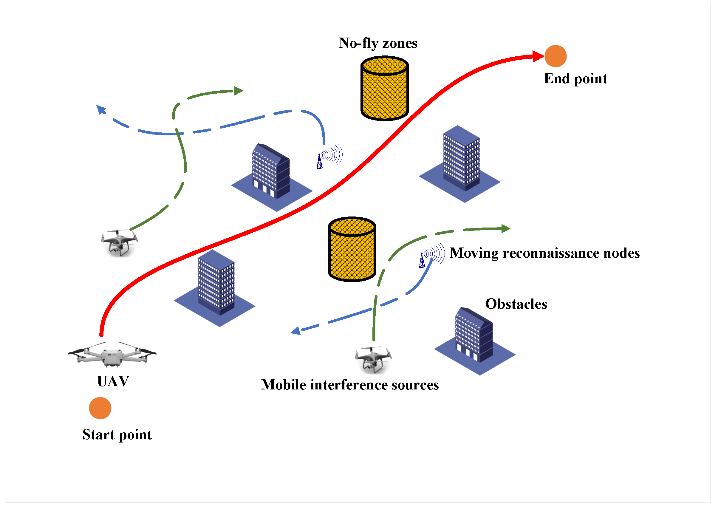
1. Introduction
- (a)
- To meet the real-time path planning requirements of UAVs in dynamic interference environments, a path planning model based on initial path guidance is proposed. This model comprehensively considers the safe flight constraints, motion characteristics of UAVs, and reconnaissance data collection constraints, establishing a trajectory optimization problem.
- (b)
- During the path planning phase, by introducing slack variables and constructing equivalent constraints, the non-convex path planning problem is transformed into a convex problem, which is then iteratively solved using SCA. The planning process takes into account the UAV motion characteristics, resulting in a final path suitable for execution by the flight control module.
- (c)
- To address the rapid replanning requirements when the positions of interference sources and reconnaissance nodes change dynamically, an initial path generation algorithm is designed based on the communication flight corridor (CFC) and collision detection correction. This algorithm guides the optimization search of SCA, thereby achieving rapid replanning of the UAV path.
- (d)
- The performance of the proposed algorithm under different parameter configurations is validated through numerical simulations, and comparisons are made with the state-of-the-art research. The results demonstrate that in scenarios where interference sources and ground reconnaissance nodes change dynamically, the proposed method exhibits high reliability and planning efficiency in solving the path planning problem with a focus on the timeliness of reconnaissance data.
2. System Model
2.1. Data Collection Channel with Interference
2.2. UAV Motion Model
2.3. Path Optimization for Reconnaissance UAVs in Dynamic Scenarios
3. Algorithm Design
3.1. Reconnaissance Node and Interference Source Position Prediction
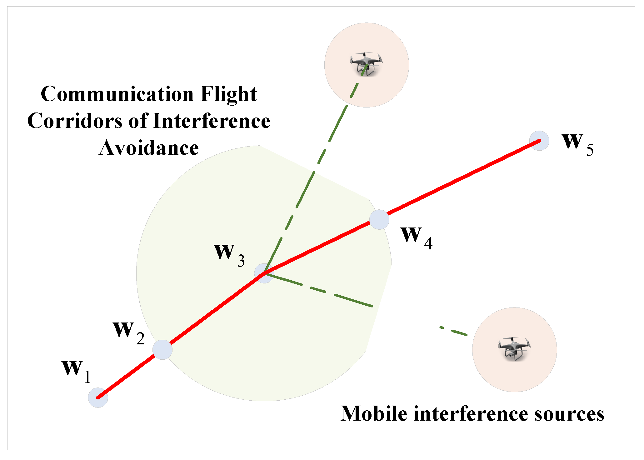
3.2. Initial Path Generation
| Algorithm 1: Initial path generation algorithm for communication flight corridors with interference avoidance. |
|
3.3. SCA-Based Path Optimization
| Algorithm 2: Path correction for obstacles and no-fly zones. |
|
| Algorithm 3: SCA path optimization based on the initial path in the communication flight corridor. |
|
| Algorithm 4: Real-time path optimization for data collection of mobile reconnaissance nodes in dynamic interference environments. |
|
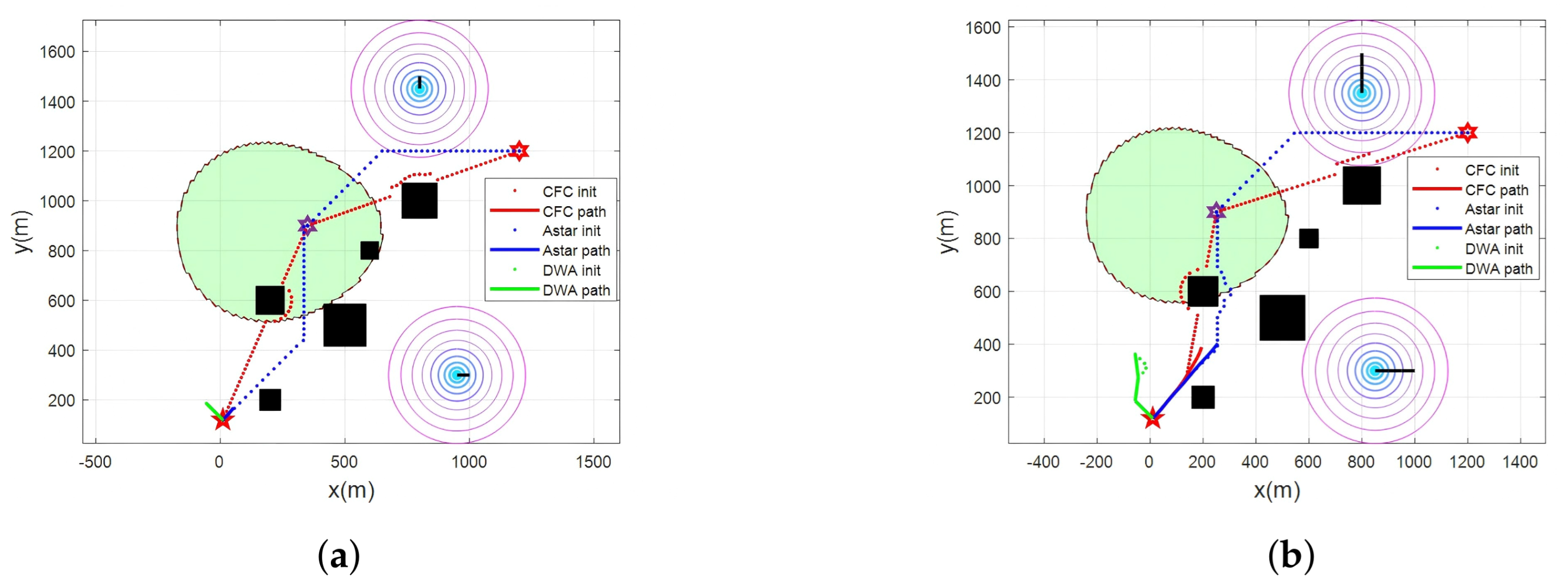
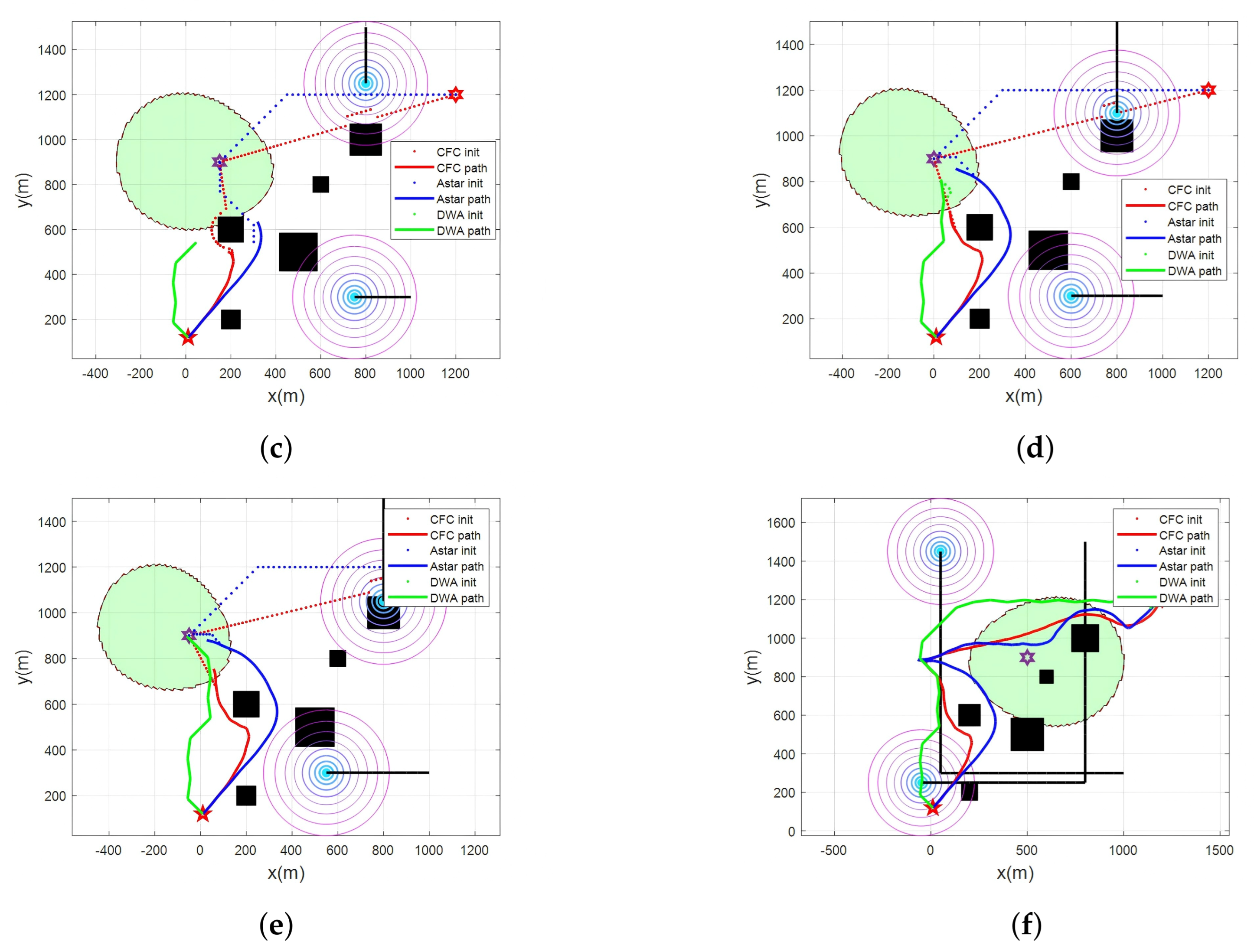
4. Numerical Results
4.1. Parameter Settings
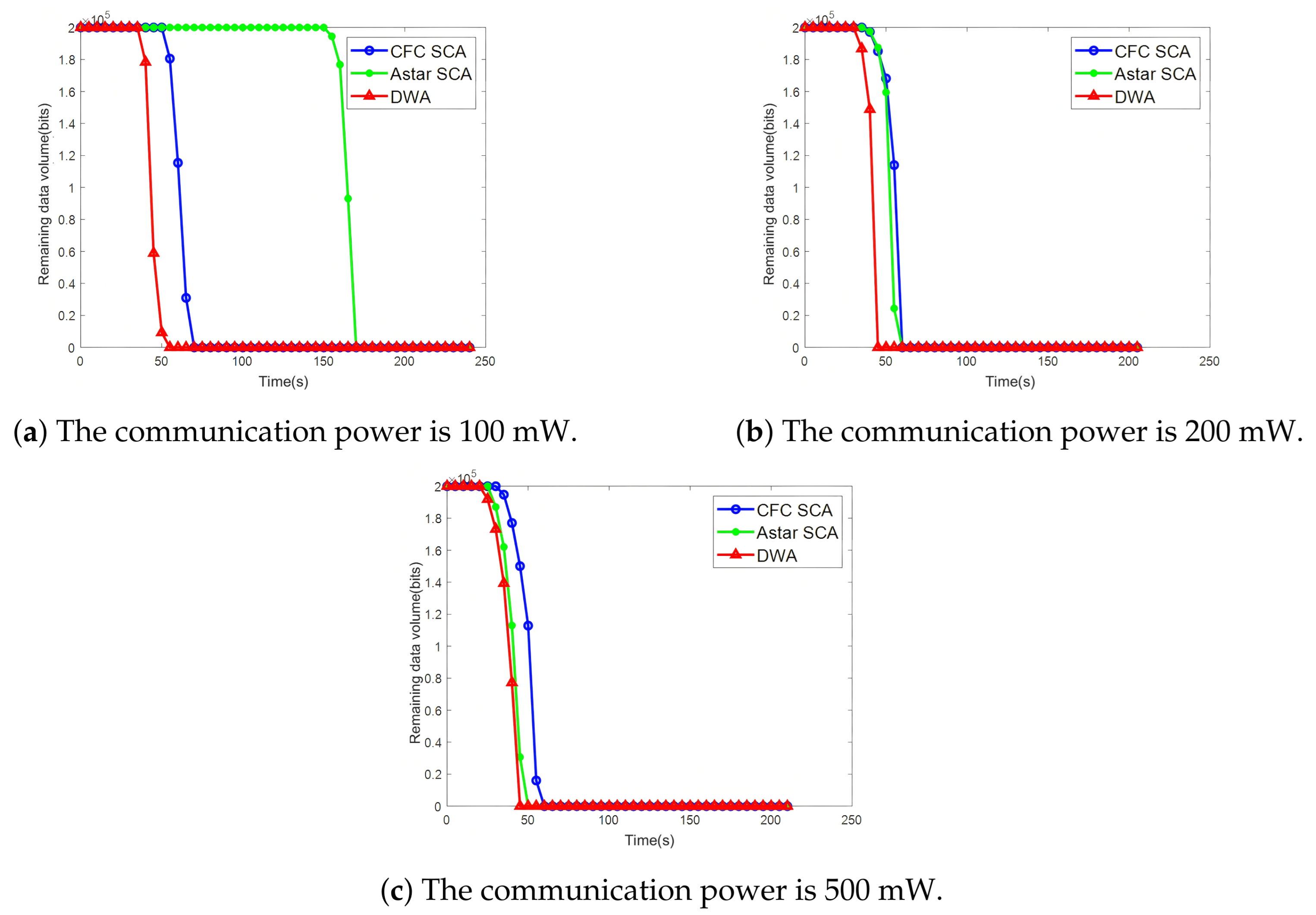
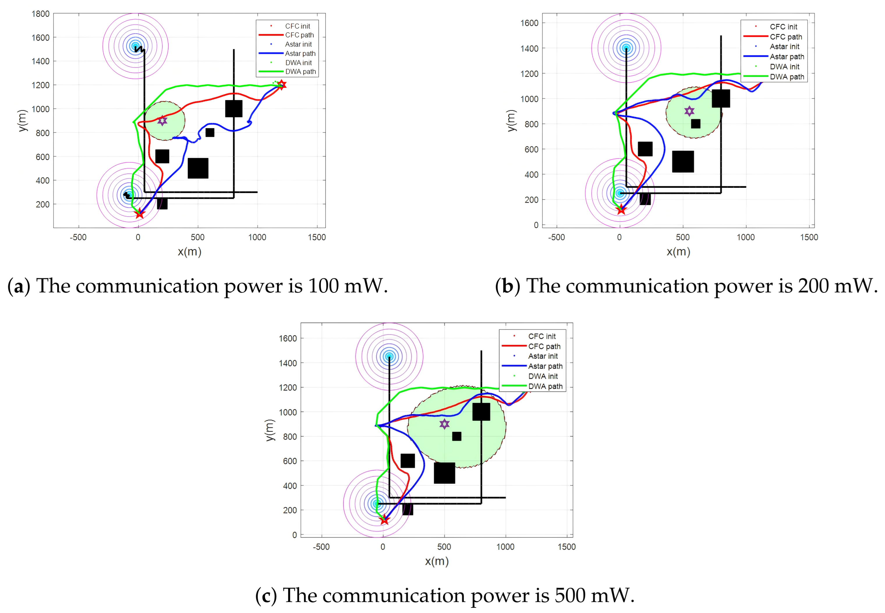
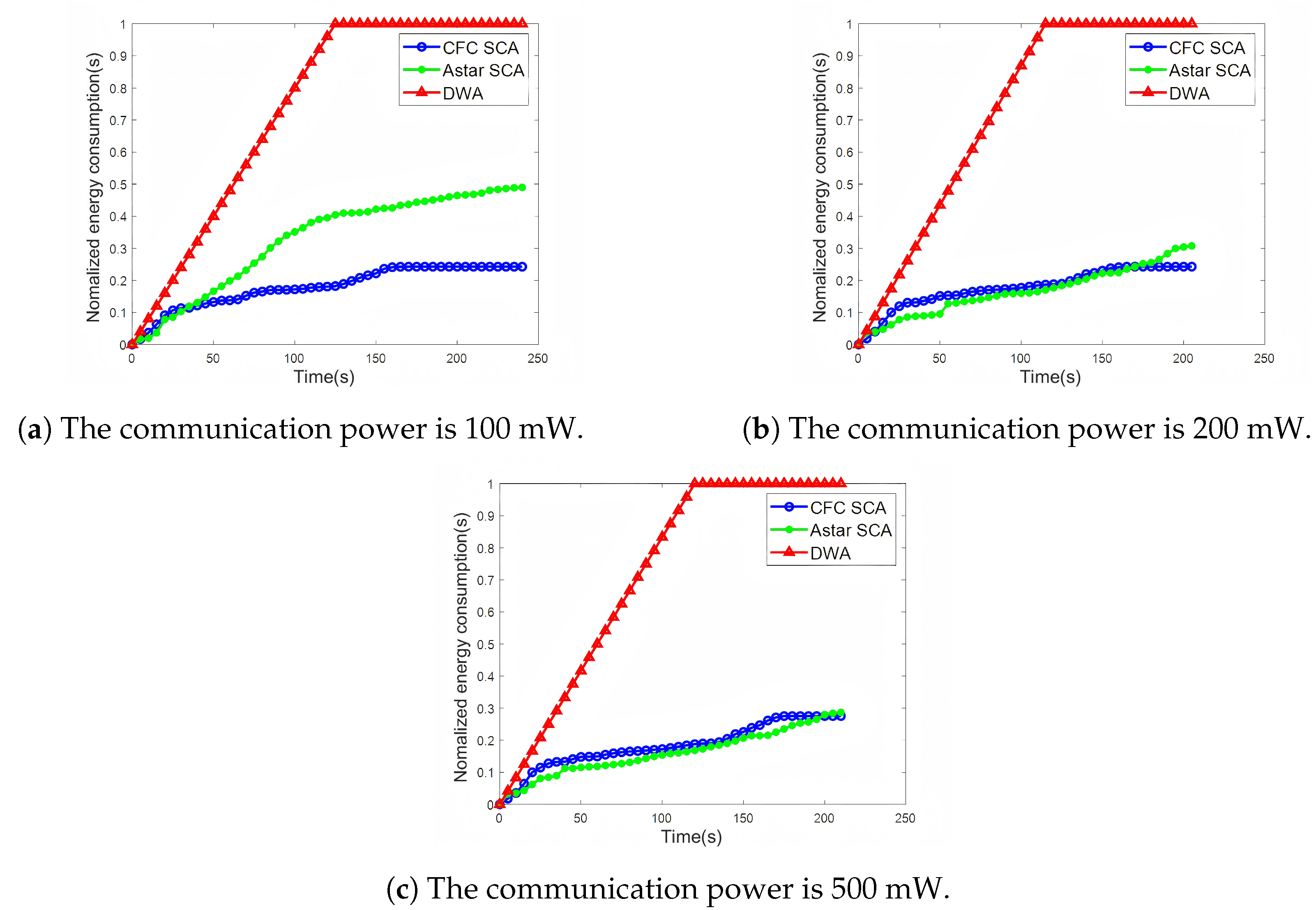
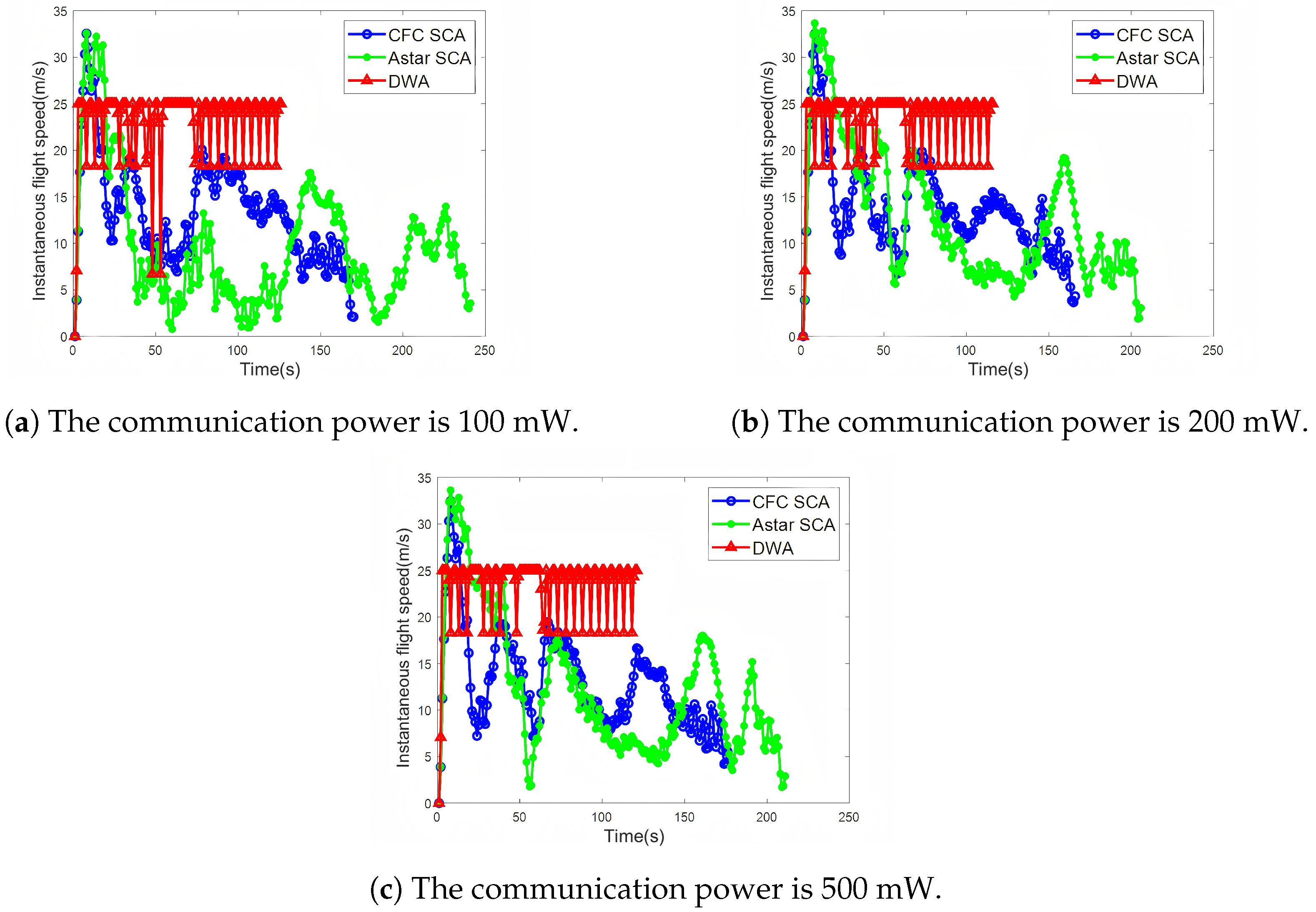
4.2. Result Analysis and Discussion
5. Conclusions
Author Contributions
Funding
Data Availability Statement
Conflicts of Interest
References
- Zhang, J.; Cui, Y.; Ren, J. Dynamic mission planning algorithm for UAV formation in battlefield environment. IEEE Trans. Aerosp. Electron. Syst. 2023, 59, 3750–3765. [Google Scholar] [CrossRef]
- Shen, L.; Wang, N.; Zhang, D.; Chen, J.; Mu, X.; Wong, K.M. Energy-aware dynamic trajectory planning for UAV-enabled data collection in mMTC networks. IEEE Trans. Green Commun. Netw. 2022, 6, 1957–1971. [Google Scholar] [CrossRef]
- Jiang, H.; Shi, W.; Chen, X.; Zhu, Q.; Chen, Z. High-efficient near-field channel characteristics analysis for large-scale MIMO communication systems. IEEE Internet Things J. 2025, 12, 7446–7458. [Google Scholar] [CrossRef]
- Ruan, C.; Zhang, Z.; Jiang, H.; Dang, J.; Wu, L.; Zhang, H. Wideband near-field channel covariance estimation for XL-MIMO systems in the face of beam split. IEEE Trans. Veh. Technol. 2025, 74, 2912–2926. [Google Scholar] [CrossRef]
- Wei, Z.; Zhu, M.; Zhang, N.; Wang, L.; Zou, Y.; Meng, Z.; Wu, H.; Feng, Z. UAV-assisted data collection for internet of things: A survey. IEEE Trans. Green Commun. Netw. 2022, 9, 15460–15483. [Google Scholar] [CrossRef]
- Li, J.; Zhao, H.; Wang, H.; Gu, F.; Wei, J.; Yin, H.; Ren, B. Joint optimization on trajectory, altitude, velocity, and link scheduling for minimum mission time in UAV-aided data collection. IEEE Internet Things J. 2020, 7, 1464–1475. [Google Scholar] [CrossRef]
- Ruan, C.; Zhang, Z.; Jiang, H.; Zhang, H.; Dang, J.; Wu, L. Simplified learned approximate message passing network for beamspace channel estimation in mmWave massive MIMO systems. IEEE Trans. Wirel. Commun. 2024, 23, 5142–5156. [Google Scholar] [CrossRef]
- Zhou, B.; Pan, J.; Gao, F.; Shen, S. RAPTOR: Robust and perception-aware trajectory replanning for quadrotor fast flight. IEEE Trans. Robot. 2021, 37, 1992–2009. [Google Scholar] [CrossRef]
- Jiang, H.; Shi, W.; Zhang, Z.; Pan, C.; Wu, Q.; Shu, F.; Liu, R.; Chen, Z.; Wang, J. Large-scale RIS enabled air-ground channels: Near-field modeling and analysis. IEEE Trans. Wirel. Commun. 2025, 24, 1074–1088. [Google Scholar] [CrossRef]
- Chen, Z.; Guo, Y.; Zhang, P.; Jiang, H.; Xiao, Y.; Huang, L. Physical layer security improvement for hybrid RIS-assisted MIMO communications. IEEE Commun. Lett. 2024, 28, 2493–2497. [Google Scholar] [CrossRef]
- Liu, S.; Watterson, M.; Mohta, K.; Sun, K.; Bhattacharya, S.; Taylor, C.; Kumar, V. Planning dynamically feasible trajectories for quadrotors using safe flight corridors in 3-D complex environments. IEEE Robot. Autom. Lett. 2017, 2, 1688–1695. [Google Scholar] [CrossRef]
- Luo, Y.; Zhuang, Z.; Pan, N.; Feng, C.; Shen, S.; Gao, F.; Cheng, H.; Zhou, B. Star-searcher: A complete and efficient aerial system for autonomous target search in complex unknown environments. IEEE Robot. Autom. Lett. 2024, 9, 4329–4336. [Google Scholar] [CrossRef]
- Wang, J.; Xiao, J.; Zou, Y.; Xie, W.; Liu, Y. Wideband beamforming for RIS assisted near-field communications. IEEE Trans. Wirel. Commun. 2024, 23, 16836–16851. [Google Scholar] [CrossRef]
- Chen, J.; Sun, J.; Wang, G. From unmanned systems to autonomous intelligent systems. Engineering 2022, 12, 16–19. [Google Scholar] [CrossRef]
- Pei, L.; Lin, J.; Han, Z.; Quan, L.; Cao, Y.; Xu, C.; Gao, F. Collaborative planning for catching and transporting objects in unstructured environments. IEEE Robot. Autom. Lett. 2024, 9, 1098–1105. [Google Scholar] [CrossRef]
- Quan, L.; Han, L.; Zhou, B.; Shen, S.; Gao, F. Survey of UAV motion planning. IET Cyber-Syst. Robot. 2020, 2, 14–21. [Google Scholar] [CrossRef]
- Liu, J.; Jayakumar, P.; Stein, J.L.; Ersal, T. A nonlinear model predictive control formulation for obstacle avoidance in high-speed autonomous ground vehicles in unstructured environments. Veh. Syst. Dyn. 2018, 56, 853–882. [Google Scholar] [CrossRef]
- Zhu, B.; Bedeer, E.; Nguyen, H.H.; Barton, R.; Henry, J. UAV trajectory planning in Wireless sensor networks for energy consumption minimization by deep reinforcement learning. IEEE Trans. Veh. Technol. 2021, 70, 9540–9554. [Google Scholar] [CrossRef]
- Zhao, Y.; Yan, L.; Xie, H.; Dai, J.; Wei, P. Autonomous exploration method for fast unknown environment mapping by using UAV equipped with limited FOV sensor. IEEE Trans. Ind. Electron. 2024, 71, 4933–4943. [Google Scholar] [CrossRef]
- Zeng, Y.; Xu, X.; Zhang, R. Trajectory design for completion time minimization in UAV-enabled multicasting. IEEE Trans. Wirel. Commun. 2018, 17, 2233–2246. [Google Scholar] [CrossRef]


| Parameter | Value |
|---|---|
| Interference power | |
| Channel bandwidth B | |
| Maximum flight speed | |
| Maximum flight acceleration | |
| Noise power spectral density | |
| Path loss factor | 2 |
| Minimum flight altitude | |
| Maximum flight altitude | |
| Carrier frequency | |
| Minimum communication rate | |
| Discrete time slot width |
Disclaimer/Publisher’s Note: The statements, opinions and data contained in all publications are solely those of the individual author(s) and contributor(s) and not of MDPI and/or the editor(s). MDPI and/or the editor(s) disclaim responsibility for any injury to people or property resulting from any ideas, methods, instructions or products referred to in the content. |
© 2025 by the authors. Licensee MDPI, Basel, Switzerland. This article is an open access article distributed under the terms and conditions of the Creative Commons Attribution (CC BY) license (https://creativecommons.org/licenses/by/4.0/).
Share and Cite
Xie, C.; Gu, C.; Wu, B.; Guo, D. Flight Path Optimization for UAV-Aided Reconnaissance Data Collection. Electronics 2025, 14, 1718. https://doi.org/10.3390/electronics14091718
Xie C, Gu C, Wu B, Guo D. Flight Path Optimization for UAV-Aided Reconnaissance Data Collection. Electronics. 2025; 14(9):1718. https://doi.org/10.3390/electronics14091718
Chicago/Turabian StyleXie, Chen, Chuan Gu, Binbin Wu, and Daoxing Guo. 2025. "Flight Path Optimization for UAV-Aided Reconnaissance Data Collection" Electronics 14, no. 9: 1718. https://doi.org/10.3390/electronics14091718
APA StyleXie, C., Gu, C., Wu, B., & Guo, D. (2025). Flight Path Optimization for UAV-Aided Reconnaissance Data Collection. Electronics, 14(9), 1718. https://doi.org/10.3390/electronics14091718