Unsupervised Specific Emitter Identification via Group Label-Driven Contrastive Learning

Abstract

Specific emitter identification (SEI), as an emerging physical-layer security authentication method, is crucial for maintaining information security in the Internet of Things. However, existing deep learning-based SEI methods require extensive labeled data for training, which are often unavailable in untrusted scenarios. Furthermore, due to the subtle nature of radio-frequency fingerprints, unsupervised SEI struggles to achieve high accuracy in identification without the guidance of labels. In this paper, we propose an unsupervised SEI method based on group label-driven contrastive learning (GLD-CL). We propose a novel method for constructing the dataset: all input samples derived from the same received signal segment are grouped together and assigned a unique identifier, termed the group label. Based on this, we improve the loss function of self-supervised contrastive learning. With the assistance of group labels, the feature vectors of the same class in the feature space become more closely clustered, enhancing the accuracy of unsupervised SEI. Extensive experimental results based on real-world datasets demonstrate that the normalized mutual information of GLD-CL achieves 96.4% accuracy, representing an improvement of 5.68% or more compared to the baseline algorithms. Furthermore, GLD-CL exhibits robust performance, achieving good identification accuracy across various signal-to-noise ratio scenarios.

1. Introduction

Specific Emitter Identification (SEI) is a physical-layer security authentication technology that identifies individual transmitting devices by leveraging unique RF fingerprints embedded within electromagnetic signals [1]. These fingerprints arise from hardware manufacturing variations in components like oscillators and amplifiers, creating distinct signal characteristics, even among identical device models [2]. As Internet of Things (IoT) deployments are projected to reach 25.1 billion connected devices by 2025, SEI offers significant advantages over traditional cryptographic methods, which face increasing vulnerability and impose computational burdens on resource-constrained IoT devices [3]. SEI authentication requires no additional hardware, remains effective against impersonation and cloning attacks due to the irreproducibility of RF fingerprints, and can be seamlessly integrated with existing security measures, making it particularly valuable for enhancing IoT information security [4,5,6].

The advent of deep learning has significantly improved the accuracy of SEI due to its powerful feature extraction capabilities. Robyns et al. [7] were among the pioneers in applying convolutional neural networks (CNNs) and multilayer perceptrons (MLPs) to SEI. Subsequently, various networks, such as residual networks (ResNet) [8,9], long short-term memory (LSTM) [10] networks, recurrent neural networks (RNNs), gated recurrent units (GRUs) [11], and transformers [12], have been utilized in SEI and have achieved promising results. Wang et al. [13] proposed the use of complex-valued neural networks for identification to better accommodate the complex form of received signals.

However, the aforementioned deep learning models all require a substantial amount of labeled data to train the identification models, which is almost infeasible in non-cooperative scenarios. In such cases, labeling a large number of signals can be prohibitively expensive. To address these challenges, researchers have explored unsupervised SEI methods that do not rely on labels. Self-supervised contrastive learning (SSCL) has emerged as an effective unsupervised learning approach and has been widely applied to achieve unsupervised SEI. Zha et al. [14] sorted unlabeled signals based on their signal-to-noise ratios (SNRs) and pre-trained the network using contrastive learning on signals with high SNRs. Finally, they employed K-means clustering to obtain the final recognition results. Shen et al. [15] utilized contrastive learning for pre-training and subsequently fine-tuned the model using a few labeled data to achieve precise identification. Hao et al. [16] proposed a bit-pulse selection strategy and several data augmentation techniques to improve the accuracy of SEI based on SSCL. Due to the subtle nature of RF fingerprint features and the high degree of similarity between signals from different emitters, achieving high identification accuracy without any label assistance is extremely challenging. Therefore, the aforementioned methods often employ fine tuning with a minimal number of labeled samples or pseudo-label-assisted approaches to enhance accuracy. However, in some situations, labeled samples may be unavailable, and the quality of pseudo-labels depends on the initial feature extraction network, which may contain numerous errors that can mislead subsequent identification.

When constructing an unsupervised SEI dataset, a received signal segment can typically be divided into multiple input samples. Since these samples originate from the same transmitted signal segment of a certain emitter, their true labels are necessarily the same, although the specific classification is unknown. Therefore, we consider them to have the same group label. In this paper, we leverage the fact that input samples from the same signal segment share the same group label to improve the loss function of SSCL. This enables the model to acquire more information about positive instances with the assistance of group labels, thereby further bringing similar feature vectors closer together and pushing dissimilar ones farther apart in the feature space. The unsupervised SEI method based on group label-driven contrastive learning (GLD-CL) proposed in this paper achieves end-to-end identification without the need for auxiliary datasets or additional hyperparameters of the number of categories.

In summary, the main contributions of our work can be summarized as follows:

• A novel unsupervised SEI method based on GLD-CL is proposed. GLD-CL eliminates the need to pre-specify the number of classes and achieves end-to-end SEI without requiring auxiliary datasets or additional hyperparameters.
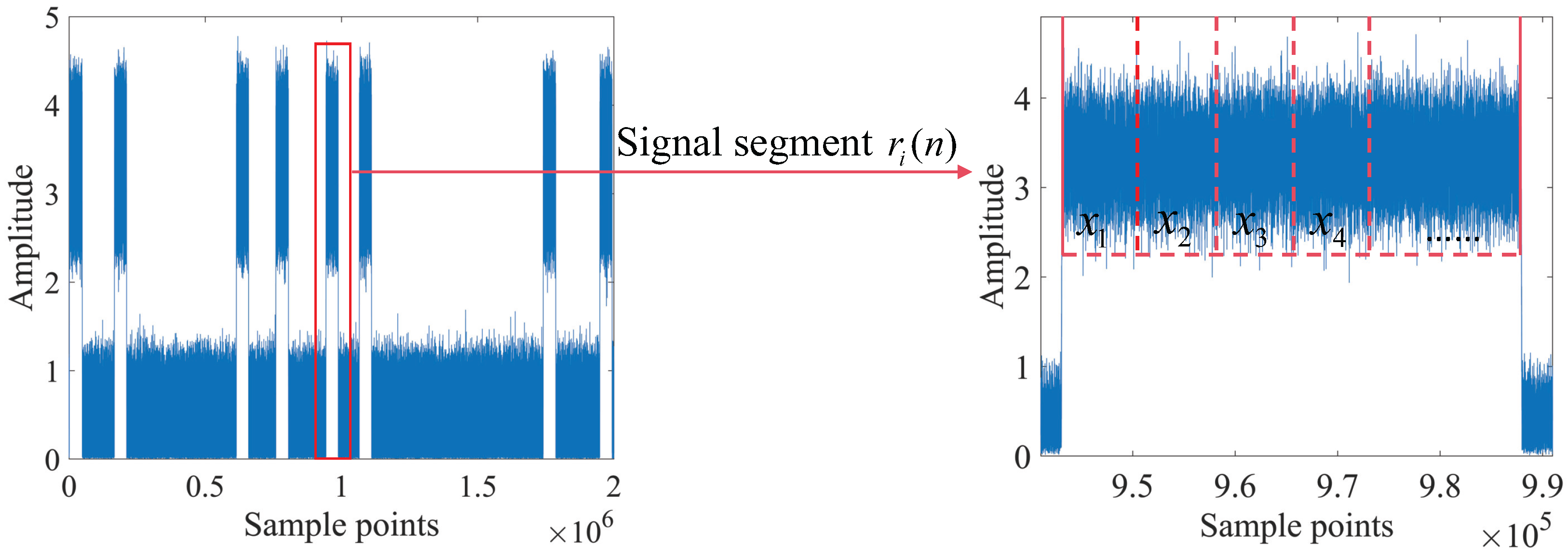
• The concept of “group label” is introduced by using the continuity of signal timing. Multiple samples obtained from the same signal segment are regarded as having the same implicit label. Using this naturally formed weak supervised information to guide the contrastive learning process, the effective expansion of positive-instance information in the feature space is realized, and the identification performance of unsupervised SEI is improved.
• Extensive experiments conducted on real-world datasets demonstrate the effectiveness of the proposed algorithm. GLD-CL achieves an improvement in identification accuracy ranging from 5.7% to 37.3% compared to baseline algorithms. Furthermore, GLD-CL exhibits robust performance, achieving good identification results across various SNR scenarios.

The rest of this paper is organized as follows: Section 2 introduces related work. The system model is presented in Section 3. The proposed GLD-CL method is introduced in Section 4. Experiments and discussions are provided in Section 5. Lastly, the conclusion is discussed in Section 6.

2. Related Work

Unsupervised SEI methods are primarily categorized into two types: generative unsupervised learning-based (GUL) methods and SSCL-based methods. GUL is an approach that performs unsupervised identification by learning the generative process of data. This methodology primarily encompasses techniques such as generative adversarial networks (GANs) and variational autoencoders (VAEs). GANs can learn complex data distributions through adversarial training, holding great promise in fields such as computer vision and natural language processing. Roy et al. [17] were the first to apply GANs to SEI. They utilized IQ imbalance in the received signals to train GANs to recognize unique high-dimensional features, achieving 99.9% accuracy in identifying counterfeit rogue transmitters. Sui et al. [18] proposed a radio-signal sorting algorithm based on subtle feature extraction using stacked autoencoders (SAEs). This algorithm achieves SEI by extracting transient features from the transmitter’s onset and frequency-changing moments through SAEs. However, GUL-based methods often get bogged down in intricate signal details, leading to overfitting. Moreover, the performance of methods combining artificial RF fingerprint features with neural networks heavily relies on the effectiveness of artificial RF fingerprint feature extraction, and the effective features may vary across different task environments.

Compared to GUL, SSCL only needs to learn to distinguish data in the feature space at the abstract semantic level, making the training optimization process simpler [16]. As a variant of contrastive learning (CL), SSCL does not rely on a large amount of manually labeled samples; instead, it leverages the inherent properties of the data to generate labels for training. The core of SSCL is to achieve self-supervised learning by constructing positive and negative instance pairs and measuring the distance between them. Specifically, positive instance pairs are usually generated by transforming the same sample, while negative instance pairs are composed of different samples. During training, the model learns effective feature representations by minimizing the distance between positive instance pairs and maximizing the distance between negative instance pairs. Zha et al. [19] employed an unsupervised method based on SSCL to extract receiver-invariant features, mitigating the impact of cross-receiver variations on identification performance. Due to the subtle nature of RF fingerprint features, signals from different transmitters are extremely similar, which may lead to poor performance when directly applying SSCL for identification. Both [15,20] and [21] adopted a subsequent fine-tuning approach using a small amount of labeled data to refine the model. However, in non-cooperative scenarios, even a minimal amount of labeled data may be unavailable. Improving the SSCL algorithm to enhance identification accuracy without relying on auxiliary datasets is crucial for promoting the application of unsupervised SEI based on SSCL.

3. System Model

3.1. Unsupervised SEI

Using techniques such as signal detection and signal separation, the received composite multi-path signals, which contain signals originating from multiple emitters, can be effectively decomposed into single-path signals in the time domain that contain only one emitter’s signal [22]. Specifically, after this processing, each signal segment uniquely corresponds to the time-domain characteristics of one emitter. After separation, the $i_{th}$ received signal segment can be represented as follows:

$$r_i\left(t\right)=H\left\{F\left[s_i\left(t\right)\right]\right\}=h\left(t\right)\ast F\left[s_i\left(t\right)\right]+w\left(t\right),$$

(1)

where $s_i\left(t\right)$ represents the ideal signal transmitted by the emitter, and $F(·)$ denotes the unintentional modulation of the signal due to the non-idealities of the emitter’s hardware, which subtly affects the amplitude, frequency, and phase of $s_i\left(t\right)$ without impeding the normal transmission and reception of the signal. $H(·)$ represents the influence of the channel, $h\left(t\right)$ denotes the channel impulse response, ∗ indicates the convolution operation, and $w\left(t\right)$ represents additive white Gaussian noise. After sampling the received signal ($r_i\left(t\right)$), we obtain the discrete-time signal ($r_i\left(n\right)$).

The goal of unsupervised SEI in this paper is to determine which emitter the signal ($r_i\left(n\right)$) originates from using the input dataset in the absence of individual labels.

From a mathematical point of view, unsupervised SEI can be expressed as the following optimization problem: In the absence of class label information, find a feature extraction function ($f_{\theta }$) such that the distance of the signals from the same emitter is minimized in the feature space while the distance of the signals from different emitters is maximized in the feature space. The problem is formally expressed as follows:

$$minL\left(f_{\theta }\right)={\mathbb{E}}_{x_i,x_j\in \mathbf{X}}[\delta (y_i,y_j)·d(f_{\theta }\left(x_i\right),f_{\theta }\left(x_j\right))-(1-\delta (y_i,y_j))·d(f_{\theta }\left(x_i\right),f_{\theta }\left(x_j\right))]$$

(2)

where $\delta (y_i,y_j)$ is the indicator function, with a value of 1 when $y_i=y_j$ and 0 otherwise; $d(·,·)$ represents the distance metric in the feature space; $\mathbf{X}$ is the input-signal sample set; and $y_i$ and $y_j$ are the true class labels of the samples (unknown in unsupervised SEI).

However, due to the nature of unsupervised learning, the value of $\delta (y_i,y_j)$ cannot be obtained directly. The concept of a group label proposed in this paper provides a weak supervision signal, which can partially replace the information of real class labels.

3.2. Group Label

The input samples for the one-dimensional neural network consist of I/Q two-channel time-domain signals. Given that the length ($l_{r_i}$) of the received signal segment ($r_i\left(n\right)$) often exceeds the predefined input sample length ($l_x$) of the neural network, each signal segment can be subdivided into m samples that meet the input specifications, as shown in Figure 1.

Since these m input samples all originate from the received signal segment ($r_i\left(n\right)$) containing only a single emitter’s time-domain signal, they necessarily belong to the same emitter. To accurately distinguish and label these samples, we propose a novel method for constructing the dataset: all input samples derived from the same received signal segment are grouped together and assigned a unique identifier, termed the group label. Specifically, input samples originating from the same received signal segment share the same group label, while samples generated from different signal segments possess distinct group labels. It is noteworthy that the granularity of the group label is finer than that of traditional individual labels. It is used solely to indicate whether samples originate from the same received signal segment. Therefore, even if two input samples have different group labels, their individual labels may still be the same, depending on whether they originate from different signal segments of the same emitter. Due to the constraints of non-cooperative scenarios, the individual labels of the data are unknown.

It is important to emphasize that group labels and individual labels (emitter labels) represent different levels of classification granularity. Individual labels directly identify specific emitters, with each emitter assigned a unique label. In contrast, group labels merely indicate whether samples originate from the same received signal segment. Multiple samples sharing the same group label are guaranteed to come from the same emitter, but samples with different group labels may still originate from the same emitter captured at different time instances. Therefore, the number of group labels typically exceeds the number of individual labels in a dataset, creating a finer granularity of classification that serves as weak supervision for the contrastive learning process without requiring knowledge of the actual emitter identities.

Based on the aforementioned grouping method, we construct the neural network input dataset ($\mathbf{X}=\{x_1,x_2,\dots ,x_N\}$) and assign it a corresponding set of group labels (${\mathbf{Y}}_g=\{y_1^1,y_2^1,\dots ,y_m^1,\dots ,y_N^M\}$). Here, N represents the total number of input samples; m denotes the number of input samples selected from each signal segment; and M is the total number of signal segments, with the relationship of $N=M\times m$. Within the same signal segment, all input samples share the same group label, i.e., $y_1^i=y_2^i=\dots =y_m^i$. For instance, label $y_j^i$ indicates that its corresponding input sample is the $j_{th}$ sample from the $i_{th}$ signal segment, and all other input samples originating from the $i_{th}$ signal segment share this group label, thereby explicitly indicating their common origin from the same emitter.

The group label approach shares conceptual similarities with several existing weakly supervised and self-labeling techniques in the broader machine learning literature while introducing important innovations specific to the RF fingerprinting domain.

Pseudo-labeling approaches typically generate artificial labels for unlabeled data based on the confident predictions of a model trained on a small labeled dataset [23]. In contrast, group labels do not rely on any labeled data or model predictions but, instead, leverage the inherent temporal structure of signal acquisition.

Our method also differs from traditional self-supervised clustering techniques like DeepCluster [24], which alternates between feature learning and cluster assignment. While DeepCluster generates pseudo-labels through clustering, our approach uses natural grouping information from the signal acquisition process itself, avoiding the instability often associated with iterative clustering procedures.

The closest analog to our approach is, perhaps, the concept of multi-instance learning (MIL), where training instances are organized in bags with bag-level labels [25]. A group label can be viewed as a bag label indicating that all samples within a group originate from the same emitter, though unlike typical MIL scenarios, we have no negative bags. However, our contrastive learning formulation introduces a novel way to leverage such weak supervision specifically for RF fingerprinting tasks, where the signal characteristics and acquisition process create natural groupings unavailable in most other domains.

4. Method

In this section, we first introduce the framework of GLD-CL. Then, the data augmentation methods and the design of the loss function for GLD-CL are discussed.

4.1. Group Label-Driven Contrastive Learning Framework for Unsupervised SEI

Unsupervised SEI refers to the discovering similarities in signals within the feature space and clustering them without the guidance of labels. Contrastive learning, by constructing similar and dissimilar samples, brings similar classes closer together and pushes different classes farther apart in the projection space, thereby achieving unsupervised identification. It has already achieved excellent results in unsupervised image recognition. However, the signal waveforms of different emitters of the same type are extremely similar, and RF fingerprints, which are subtle feature differences in signals, are even more difficult to extract compared to images. To address this challenge, we propose an unsupervised SEI algorithm based on GLD-CL. The framework of GLD-CL is shown in Figure 2 and Algorithm 1.

Algorithm 1 GLD-CL Framework for Unsupervised SEI.

Require: Dataset $\mathbf{X}=\{x_1,x_2,\dots ,x_N\}$, group labels ${\mathbf{Y}}_g=\{y_1^1,y_2^1,\dots ,y_m^1,\dots ,y_N^M\}$, feature extractor $f_{\theta }$, projection network $J_{\theta }$, maximum number of training epochs O. Ensure: individual labels for each signal sample // Data augmentation  1: for $i=1$ to N do  2:    Apply data augmentation (PR, CS, RNA) to $x_i$ to get ${\tilde{x}}_i$ and ${\tilde{x}}_{j\left(i\right)}$  3:    $\tilde{\mathbf{X}}\leftarrow \tilde{\mathbf{X}}\cup \{{\tilde{x}}_i,{\tilde{x}}_{j\left(i\right)}\}$  4: end for // Train the feature extractor and the projection network  5: for epoch = 1 to O do  6:    for each batch $\mathbf{B}\subset \tilde{\mathbf{X}}$ do  7:      Compute feature vectors $\mathbf{F}\leftarrow f_{\theta }\left(\mathbf{B}\right)$  8:      Compute projection vectors $\mathbf{Z}\leftarrow g_{\varphi }\left(\mathbf{F}\right)$  9:      Compute GLD-CL loss ${\mathcal{L}}^g$, according to Equation (8) 10:     Update $f_{\theta }$ and $J_{\theta }$ by minimizing ${\mathcal{L}}^g$ 11:    end for 12: end for // Cluster 13: Extract feature vectors for all samples ${\mathbf{F}}_{all}\leftarrow f_{\theta }\left(\tilde{\mathbf{X}}\right)$ 14: Apply DBSCAN on ${\mathbf{F}}_{all}$ to obtain clusters 15: Assign cluster labels to original dataset $\mathbf{X}$ 16: return Individual labels for each signal sample

4.1.1. Data Augmentation

Data augmentation is applied to the sample ($x_i$) using techniques such as phase rotation (PR), cyclic shifting (CS), and random noise addition (RNA), resulting in two augmented samples: ${\tilde{x}}_i$ and ${\tilde{x}}_{j\left(i\right)}$. For a dataset containing N samples, with each group consisting of m samples, after data augmentation, we obtain a dataset of size $2N$. $G=\{{\tilde{x}}_i^l,{\tilde{x}}_{j\left(i\right)}^l,\dots ,{\tilde{x}}_{i+m-1}^l,{\tilde{x}}_{j+m-1(i+m-1)}^l\}$ represents a set of $2m$ positive instances, while the remaining $2N-2m$ instances are considered negative instances. ${\tilde{x}}_i^l$ and ${\tilde{x}}_{j\left(i\right)}^l$ represent the relevant samples formed by the same sample after data augmentation.

4.1.2. Feature Extractor

The two positive instances are input into a feature extractor with shared weights, which maps the time-domain signals into a pair of 4096-dimensional feature vectors. The structure of the feature extractor proposed in this paper is based on the ResNet18 architecture, which has been widely used for supervised SEI.

4.1.3. Projection Network

An MLP is used to map the feature vectors into 128-dimensional projection vectors. The projection network reduces the dimensionality of the feature vectors, which is more conducive to the calculation of the loss function and avoids model collapse. The MLP structure used in this paper consists of a linear layer, a ReLU activation function, and another linear layer.

4.1.4. Cluster

After training is completed, the outputs from the feature extractor are extracted and clustered using DBSCAN to obtain the final identification results.

4.2. Data Augmentation

The commonly utilized data augmentation techniques in the field of image recognition, such as flipping, rotation, scaling, and cropping, are not well-suited for the processing of one-dimensional signal data. Taking into account the complex form of received signals, we employ three methods—PR, CS, and RNA—to generate augmented samples.

4.2.1. Phase Rotation

The I/Q components of the sample ($x_i\left(n\right)$) can be represented as follows:

$$x_i\left(n\right)=I+jQ,$$

(3)

where j denotes an imaginary unit. After applying phase rotation to the sample $x_i\left(n\right)$, the augmented sample (${\tilde{x}}_i\left(n\right)$) can be represented as follows:

$$\begin{array}{cc}\hfill {\tilde{x}}_i\left(n\right)& =(I+jQ)e^{j{\displaystyle \frac{\pi }{2}}\alpha }\hfill \\ & =(Icos{\displaystyle \frac{\pi }{2}}\alpha -Qsin{\displaystyle \frac{\pi }{2}}\alpha )+j(Isin{\displaystyle \frac{\pi }{2}}\alpha +Qcos{\displaystyle \frac{\pi }{2}}\alpha ),\hfill \end{array}$$

(4)

where $\alpha$ is used to control the rotation angle and, in this paper, $\alpha$ is randomly selected from the set of $[0,1,2,3]$. A schematic diagram of PR is shown in Figure 3.

4.2.2. Circular Shifting

The first $l_{cs}$ bits of the sample ($x_i\left(n\right)$) are moved to the rightmost position of the sample. The shifted sample can be represented as follows:

$$\begin{array}{cc}{\tilde{x}}_i\left(n\right)=\hfill & [x_i(l_{cs}+1),x_i(l_{cs}+2),\dots ,\hfill \\ \hfill & x_i\left(l_x\right),x_i\left(1\right),x_i\left(2\right),\dots ,x_i\left(l_{cs}\right)]\hfill \end{array}$$

(5)

where $l_{cs}$ denotes the number of shifted sampling points, $l_x$ represents the length of sample $x_i\left(n\right)$, and $x_i\left(j\right)$ denotes the value of the $j_{th}$ sampling point in sample $x_i\left(n\right)$. A schematic diagram of CS is shown in Figure 4.

4.2.3. Random Noise Addition

To introduce subtle variations in amplitude, additive white Gaussian noise (AWGN) is added to sample $x_i\left(n\right)$. The noised sample can be represented as follows:

$${\tilde{x}}_i\left(n\right)=x_i\left(n\right)+w\left(n\right),$$

(6)

where $w\left(n\right)$ represents AWGN. In this paper, the SNR for noise addition is set to 8–10 dB.

4.3. Loss Function

4.3.1. SSCL Loss Function

In SSCL, the initial dataset ($\mathbf{X}=\{x_1,x_2,\dots ,x_N\}$) undergoes a process of data augmentation to generate an expanded dataset comprising $2N$ instances, denoted as $\tilde{\mathbf{X}}=\{{\tilde{x}}_1,{\tilde{x}}_2,\dots ,{\tilde{x}}_N,{\tilde{x}}_{N+1\left(1\right)},{\tilde{x}}_{N+2\left(2\right)},\dots ,{\tilde{x}}_{2N\left(N\right)}\}$. The most commonly used loss function in SSCL is the InfoNCE loss, which is calculated according to the following equation:

$${\mathcal{L}}^{self}=\sum _{i=1}^{2N}{\mathcal{L}}_i^{self}=-\sum _{i=1}^{2N}log{\displaystyle \frac{exp(z_i·z_{j\left(i\right)}/\tau )}{{\displaystyle \sum _{a\in A\left(i\right)}}exp(z_i·z_a/\tau )}},$$

(7)

where $z_i$ and $z_{j\left(i\right)}$ are the projection vectors of the positive pair (${\tilde{x}}_i$ and ${\tilde{x}}_{j\left(i\right)}$, respectively). ${\tilde{x}}_i$ is also known as the anchor. The “·” symbol denotes the inner product, $\tau \in R^{+}$ is the temperature hyperparameter, $i\in I_n=\{1,2,\dots ,2N\}$ is the index of the augmented sample, and $A\left(i\right)=I_n\setminus \left\{i\right\}$.

4.3.2. GLD-CL Loss Function

Samples sharing the same group label are also considered positive instances. Consequently, the number of positive instances expands from 2 to $2m$. The incorporation of group labels enriches the form of positive instances and aligns more closely with real-world signals. Based on Equation (7), we present the loss function of GLD-CL:

$$\begin{array}{cc}{\mathcal{L}}^g\hfill & ={\displaystyle \sum _{i=1}^{2N}}{\mathcal{L}}_i^g\hfill \\ \hfill & ={\displaystyle \sum _{i=1}^{2N}}{\displaystyle \frac{-1}{2m-1}}{\displaystyle \sum _{p\in P\left(i\right)}}log{\displaystyle \frac{exp(z_i·z_p/\tau )}{{\displaystyle \sum _{a\in A\left(i\right)}}exp(z_i·z_a/\tau )}},\hfill \end{array}$$

(8)

where $P\left(i\right)=\{p\in A\left(i\right):y_p^g=y_i^g\}$ denotes the index set of all positive instances, excluding i, that share the same group, and $(2m-1)$ represents the cardinality of set $P\left(i\right)$.

From a theoretical perspective, the GLD-CL loss function significantly enhances clustering effects in the feature space by introducing group label information. Traditional SSCL only treats augmented versions of the same sample as positive pairs, lacking constraints on the relationships between different samples of the same class. Our method, however, explicitly treats all samples from the same signal segment as positive samples, which is equivalent to adding extra attractive forces in the feature space.

Specifically, for each anchor sample ($x_i$), traditional SSCL has only one positive sample ($x_{j\left(i\right)}$) mutually attracting in the feature space, whereas GLD-CL provides $2m-1$ positive samples for each anchor sample, which collectively form a stronger clustering gravitational field. Mathematically, the increase in the numerator term (${\sum }_{p\in P\left(i\right)}exp(z_i·z_p/\tau )$) in Equation (8) means that feature vectors within the same group are pulled together more strongly. According to contrastive learning theory [26], this introduction of multiple positive samples not only increases the strength of the learning signal but also reduces the bias that might result from a single positive sample.

Furthermore, when the number of groups (M) is much larger than the actual number of emitters (K$(M>>K)$), many samples with different group labels actually come from the same emitter. During training, although these samples are treated as negative samples, their feature representations tend to become similar. Through the iterative optimization process, this similarity causes samples that originally belong to the same class but have different group labels to gradually gather in nearby regions of the feature space, forming a clustering structure that reflects the true emitter categories. This theoretical mechanism explains why GLD-CL can achieve tighter clustering effects without real class labels. Equation (8) possesses the following properties:

• It can be generalized to multiple positive sample pairs: In contrast to Equation (7), both the augmented samples and all samples sharing the same group label contribute to the numerator. The GLD-CL loss provides tightly aligned representations for all samples with the same group label, reducing the uncertainty between different samples, thereby generating a more robust clustering feature space than the SSCL loss.
• The more negative instances, the stronger the contrastive performance: The denominator of Equation (8) includes the summation of similarities between the anchor and all negative instances, which is consistent with SSCL loss. The more negative instances there are, the more hard negatives are available during contrast, which is more conducive to increasing the distance between the feature vectors of positive and negative instances [27].
• It possesses the ability to mine hard positive/negative instances: Hard positive instances refer to those that share the same label as the anchor but are deemed dissimilar by the model. Hard negative instances, on the other hand, are those that have a different label from the anchor but are incorrectly considered similar by the model. Conversely, samples where the model’s identification aligns with the label are termed easy positive/negative instances. In contrastive learning, mining hard positive/negative instances is crucial for enhancing the model’s discriminative power and generalization ability. Equation (8) inherently possesses the ability to mine hard positive/negative instances without additional strategies. During training, the loss function automatically assigns greater weights to those pairs of samples that are difficult to distinguish (i.e., hard instances), as they contribute more significantly to the loss value.

The mathematical proof of the properties of Equation (8) can be found in Appendix A.

5. Experiments and Discussion

5.1. Dataset and Data Preprocessing

In this section, we conducted extensive experiments on the CC2530 and ADS-B datasets to validate the performance of the proposed GLD-CL.

5.1.1. Dataset

(1)

CC2530

We collected signals from nine Zigbee devices, specifically the CC2530 type, using a BB60C receiver. The Zigbee device CC2530 is manufactured by EBYTE in Shenzhen, China, and BB60C is manufactured by Signal Hound in Seattle, USA. The CC2530, designed as a low-power system-on-a-chip (SoC), is widely used in sensor networks and the IoT. It operates based on the IEEE 802.15.4 [28] protocol, with a carrier frequency of 2.4 GHz. The sampling rate of the receiver was set to 20 MHz, which is oversampled, to retain more time-domain information.

Based on the varying number of samples per group, we set up six different ways to construct datasets, ranging from 1 to 6 samples per group. The total number of samples across all configurations remains consistent, with 600 input samples collected from each emitter. The sole difference lies in the assignment of group labels.

(2)

ADS-B [29]

The ADS-B signal is the wireless signal broadcast by aircraft to the ground and other aircraft, including its position, altitude, speed, and other information, which is used to monitor the position and status of the aircraft in real time. The signal frequency is usually 1090 MHz. The dataset contains I/Q signals from 100 civil aircraft; each aircraft has 400 samples, and the signals of 15 of them are selected as identification targets. Dataset construction is the same as for CC2530.

5.1.2. Data Preprocessing

To mitigate the impact of channel noise on identification accuracy, we employed wavelet denoising. Based on experimental testing, the wavelet basis function selected in this paper is “db4”, with a fixed threshold estimation method and a decomposition level of 4. Wavelet denoising can improve the SNR of signals by approximately 8 dB.

5.2. Implementation Details and Evaluation Metrics

5.2.1. Implementation Details

The optimizer for the feature extractor is the Adam optimizer, with the initial learning rate set to 0.0003 and a learning rate adjustment mechanism configured as StepLR. All experiments were conducted on a single NVIDIA RTX 3080 Ti graphics card (Gigabyte Corporation, Taipei, China). The temperature hyperparameter was set to 1. All codes were executed on Pytorch version 2.1.2. The parameter summary is shown in

Table 1. Summary of hyperparameters used in experiments.

Hyperparameter	Value
Batch size	1024
Learning rate	0.0003
Learning rate schedule	StepLR
Optimizer	Adam
Group size (default)	3
Input sample length (default)	2 × 1024

.

5.2.2. Evaluation Metrics

To comprehensively evaluate the performance of the proposed algorithm, we adopted three commonly used clustering metrics: normalized mutual information (NMI), the adjusted Rand index (ARI), and the Fowlkes–Mallows index (FMI). The value range for NMI and FMI is [0, 1], while the value range for ARI is [−1, 1]. For all these metrics, a higher value indicates better performance.

5.3. Performance Comparison with Existing Methods

We compared GLD-CL with existing typical unsupervised SEI methods, including k-means [30], DBSCAN [31], SAE [18], deep adaptive clustering (DAC) [32], deep transfer clustering (DTC) [33], RFFE-infoGAN [34], and signal-contrastive self-supervised clustering (SCSC) [16]. The following is a brief introduction to these comparison algorithms.

• SAE is composed of multiple autoencoder layers stacked together. It learns higher-level features by minimizing the reconstruction error between the input and output of the entire stacked autoencoder.
• DAC recasts the clustering problem into a binary pairwise classification framework to judge whether pairs of images belong to the same clusters.
• DTC first pretrains the model based on an auxiliary dataset, then enhances the model’s feature extraction capabilities using transfer learning and, finally, employs it to cluster samples in the target dataset.
• RFFE-infoGAN uses a GAN to extract distinguishable structured multimodal latent vectors, thereby achieving unsupervised SEI.
• SCSC uses a 1D fingerprint pyramid feature extractor to obtain hierarchical subtle features of emitter signals and generates cluster preference representations in an SSCL manner.

These methods all use raw I/Q data as input, without the need for manual extraction of expert features. The input sample length is $2\times 1024$, and each group has three samples. For DAC and DTC, which require auxiliary datasets for model pretraining, samples from 9 additional CC2530 devices collected in the same manner and 15 separate ADS-B signals were used as the auxiliary datasets. To ensure their appropriate application to 1D RF signals, we modified the feature extraction networks in both DAC and DTC by replacing 2D convolutional layers with 1D convolutional layers that are better suited for processing RF time-series data. For the clustering stage of the approach, the DBSCAN algorithm was utilized with parameters of $\epsilon =4$ and $MinPts=10$. These parameters were selected using the k-distance graph method, which involves plotting the distance of each point to its $k_{th}$ nearest neighbor in ascending order and identifying the “elbow point” that indicates a suitable $\epsilon$ value. The MinPts value was chosen to balance noise filtering with the ability to detect smaller legitimate clusters, representing approximately 1% of the dataset size. The high-quality feature representations learned by the GLD-CL method made the clustering results relatively stable across reasonable parameter ranges.

Table 2. Performance comparison with other methods.

Dataset	Method	NMI	ARI	FMI
CC2530	K-means	0.1817	0.2525	0.3609
	DBSCAN	0.3859	0.3331	0.4706
	SAE	0.5909	0.3939	0.5913
	DAC	0.7421	0.5755	0.6587
	DTC	0.8122	0.7043	0.7048
	RFFE-infoGAN	0.8846	0.7379	0.7916
	SCSC	0.9072	0.9053	0.9155
	SSCL+k-means	0.8487	0.7315	0.7658
	SSCL+DBSCAN	0.8851	0.7989	0.8138
	GLD-CL+k-means (ours)	0.8592	0.7269	0.7694
	GLD-CL+DBSCAN (ours)	0.9641 1	0.9614	0.9659
ADS-B	K-means	0.1468	0.1837	0.2713
	DBSCAN	0.3068	0.2643	0.3875
	SAE	0.4952	0.3141	0.4721
	DAC	0.6475	0.4578	0.5382
	DTC	0.7393	0.6015	0.6224
	RFFE-infoGAN	0.8032	0.6462	0.6947
	SCSC	0.8724	0.8509	0.8691
	SSCL+k-means	0.7789	0.6381	0.6818
	SSCL+DBSCAN	0.8143	0.7037	0.7354
	GLD-CL+k-means (ours)	0.8353	0.7148	0.7278
	GLD-CL+DBSCAN (ours)	0.9286	0.9255	0.9229

¹ The bold font indicates the optimal performance.

presents the identification results for the 9 CC2530 and 15 ADS-B devices, where the number of group labels in our method is set to three per group. It can be observed that our proposed method demonstrates a clear advantage in identification performance. Compared to DTC, GLD-CL improves NMI and ARI by 7.19% and 22.35% on the CC2530 dataset, respectively. Compared to SCSC, GLD-CL enhances NMI and ARI by 2.45% and 3.61% on the CC2530 dataset, respectively. Due to the increase of the number of emitters to be identified, the identification performance of the proposed method on the ADS-B dataset is slightly reduced, but it is still better than that of the comparison method. Furthermore, the metrics of the proposed method are more stable, proving its superior individual identification performance. The identification performance of the proposed method is superior to that of all compared methods, effectively improving its reliability as an identity verification method. Figure 5 shows the performance of GLD-CL in the feature space on the CC2530 dataset.

5.4. Component-Wise Ablation Experiment

To better understand the individual contributions of each component in the proposed method, we conducted a systematic ablation experiment, isolating the effects of (1) the GLD-CL loss function (which inherently incorporates a group labeling strategy) and (2) data augmentation techniques. All experiments were performed on the CC2530 dataset with a group size of three and a sample length of 2 × 1024.

As shown in

Table 3. Component-wise ablation study results.

Model Configuration		NMI
GLD-CL Loss Function	Data Augmentation
	√	0.8851
√		0.1912
√	√	0.9641

, each component contributes significantly to the overall performance improvement. Data augmentation is the foundation of contrastive learning, and without any data augmentation methods, the model’s identification performance is extremely poor, with almost no individual identification ability. The specific impacts of different data augmentation methods are described in detail in Section 5.8.

Incorporating the GLD-CL loss function as described in Section 4.3.2 yields a substantial improvement (7.9% increase in NMI). This demonstrates that explicitly leveraging group label information in the contrastive learning objective is the core contribution of our approach and the primary driver of performance gains.

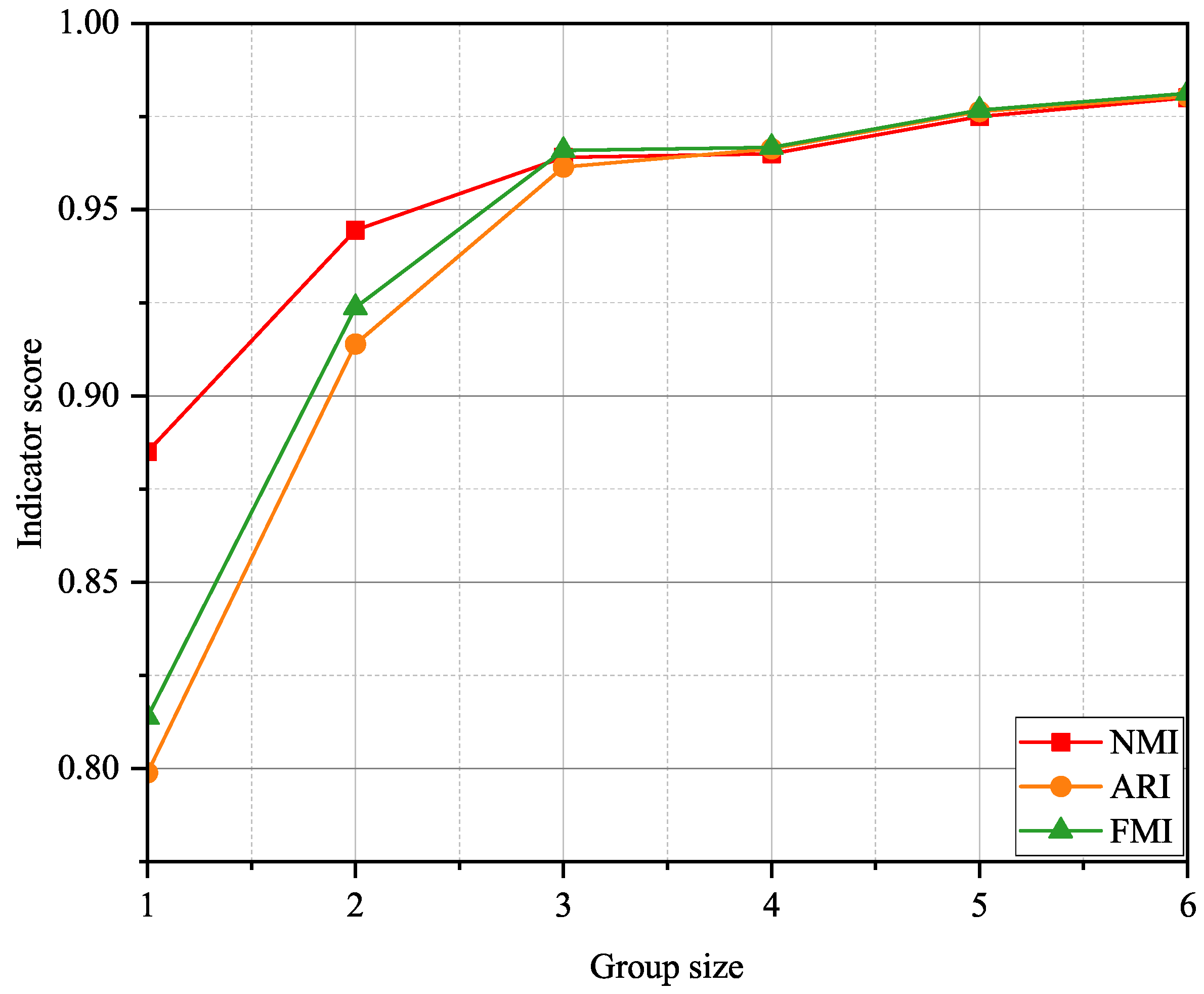
5.5. Performance Comparison of Different Group Sizes

To further validate the effectiveness of group labels in improving performance, we investigated the impact of varying the number of samples per group on performance with the CC2530 dataset. Results are presented in Figure 6. The input sample length was set to $2\times 1024$. The case in which each group contains only one sample, denoted as $m=1$, corresponds to conventional SSCL. As the number of samples per group increases, the identification performance improves, indicating a larger number of samples per group and, consequently, more positive instances, facilitating the feature extractor in bringing similar instances closer together. This observation aligns with Equation (8).

5.6. Performance Comparison Under Different SNRs

We conducted performance evaluations of GLD-CL under varying SNR conditions using nine CC2530 emitters. The input sample length was $2\times 1024$, and each group had three samples. As shown in Figure 7, GLD-CL maintains high performance, even under −10 dB. When the SNR exceeds 0 dB, the NMI of identification results remains above 90%. Furthermore, when the SNR is greater than 5dB, all performance metrics surpass 95%, indicating that the method proposed in this paper is adaptable to a wide range of SNR scenarios. This effectively extends the operational range of SEI systems.

5.7. Performance Comparison of Different Sample Lengths

In this paper, we adopt a default input sample length of $2\times 1024$. If the input sample is too short, it contains insufficient information to extract distinctive RF fingerprint features. Conversely, a long input sample would result in an excessive computational load for the feature extractor and impose high requirements on memory capacity. To validate the rationality of our chosen input sample length, we conducted experiments to assess the impact of varying input sample lengths on identification performance using the CC2530 dataset. Except for the experiment with a sample length of $2\times 2048$, where the batch size was set to 512 due to memory constraints, all other experiments were conducted with a batch size of 1024, and the number of group labels were set as three per group. The experimental results, as presented in

Table 4. Performance comparison of different sample lengths.

Sample Length	NMI	ARI	FMI
128	0.594	0.3674	0.4167
256	0.7043	0.5726	0.6714
512	0.7844	0.6397	0.7115
1024	0.964 1	0.9614	0.9659
2048	0.9504	0.9594	0.9526

¹ The bold font indicates the optimal performance.

, demonstrate that identification performance gradually improves as the input sample length increases. However, the performance slightly decreased from $2\times 1024$ to $2\times 2048$. This is because an input sample length of $2\times 1024$ already encapsulates sufficient fine-grained features. Additionally, constrained by memory capacity, we had to reduce the batch size for the $2\times 2048$ experiment. In the context of contrastive learning, a larger batch size provides more negative instances, which is beneficial for feature representation learning [35]. Therefore, we selected $2\times 1024$ as the default input sample length, as it strikes a balance between performance and memory requirements.

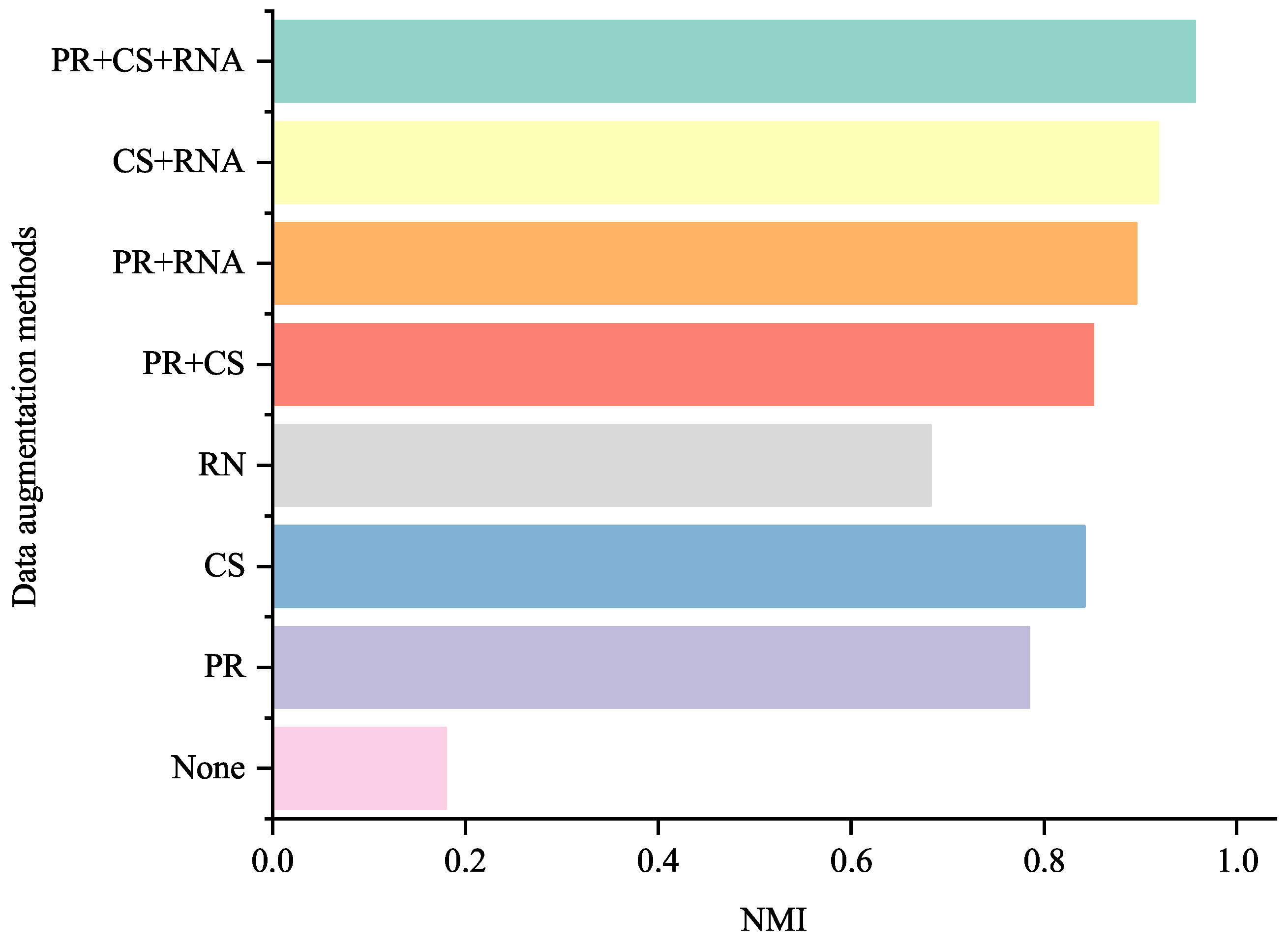
5.8. Performance Comparison of Different Data Augmentation Methods

Although GLD-CL is assisted by group labels, its effectiveness still largely depends on the use of data augmentation methods. Therefore, we conducted a thorough experimental analysis of the effectiveness of each one-dimensional data augmentation method and their combinations on the CC2530 dataset. The input sample length was $2\times 1024$, and each group had three samples. The results are shown in Figure 8.

When no data augmentation methods are employed, the two samples in a positive pair are identical, leading to poor identification performance. The identification performance is significantly improved when even a single data augmentation method is applied. Among the three data augmentation methods, CS and PR outperform RNA, with CS yielding the best results. This is because CS and PR only alter the timing relationship of the signals, with almost no loss of signal information. In contrast, RNA modifies the signal amplitude, which we believe results in information loss. Since RF fingerprints are extremely subtle features, even minor changes to the signal amplitude can impact the extraction of these fingerprints.

When multiple data augmentation methods are combined, the identification performance surpasses that of a single data augmentation method. Among the combinations of two data augmentation techniques, the combination of CS and RNA yields the best performance. When all three data augmentation techniques are used simultaneously, the optimal performance is achieved. Therefore, multiple data augmentation techniques should be employed to enhance the diversity of augmented samples and avoid the single-feature dependency that may arise from using a single data augmentation method.

6. Conclusions

In this paper, we enhanced the identification performance of unsupervised SEI based on self-supervised contrastive learning by introducing the concept of group labels, addressing the challenge of unlabeled emitter signals in non-cooperative environments. We reorganized the dataset construction approach by leveraging the prior knowledge that input samples originating from the same signal segment must share the same true label. Additionally, we improved the loss function to enable it to utilize group label information, thereby minimizing the intra-class distance and maximizing the inter-class distance of feature vectors. Extensive experiments demonstrate the high levels of robustness and effectiveness of our method, significantly outperforming existing benchmark methods.

Despite these achievements, the proposed method assumes successful signal separation, and challenges such as signal overlaps and multi-source interference remain outside the scope of the current work. Future work will focus on integrating advanced signal separation techniques to address these issues and enhance performance in dynamic RF environments. Meanwhile, our approach has limitations regarding computational efficiency. The current implementation does not fully consider the computational constraints of edge devices, which may hinder practical deployment in resource-limited scenarios. Future work should focus on incorporating model compression techniques such as pruning, quantization, and knowledge distillation to reduce the computational complexity and memory footprint of our model. This improvement would enhance the practicality of our method as a physical-layer authentication solution for IoT and other edge computing environments, where computational resources are severely constrained but security requirements remain critical. With these enhancements, we believe our approach has great potential and broad application prospects in practical wireless security systems.

References

1. Li, D.; Qi, J.; Hong, S.; Deng, P.; Sun, H. A Class-Incremental Approach with Self-Training and Prototype Augmentation for Specific Emitter Identification. IEEE Trans. Inf. Forensics Secur. 2024, 19, 1714–1727. [Google Scholar] [CrossRef]
2. Li, D.; Shao, M.; Deng, P.; Hong, S.; Qi, J.; Sun, H. A Self-Supervised-Based Approach of Specific Emitter Identification for the Automatic Identification System. IEEE Trans. Cogn. Commun. Netw. 2024, 1317–1322. [Google Scholar] [CrossRef]
3. Sauter, T.; Treytl, A. IoT-Enabled Sensors in Automation Systems and Their Security Challenges. IEEE Sensors Lett. 2023, 7, 1–4. [Google Scholar] [CrossRef]
4. Jiang, H.; Shi, W.; Chen, X.; Zhu, Q.; Chen, Z. High-Efficient Near-Field Channel Characteristics Analysis for Large-Scale MIMO Communication Systems. IEEE Internet Things J. 2025, 12, 7446–7458. [Google Scholar] [CrossRef]
5. Jiang, H.; Shi, W.; Zhang, Z.; Pan, C.; Wu, Q.; Shu, F.; Liu, R.; Chen, Z.; Wang, J. Large-Scale RIS Enabled Air-Ground Channels: Near-Field Modeling and Analysis. IEEE Trans. Wirel. Commun. 2025, 24, 1074–1088. [Google Scholar] [CrossRef]
6. Chen, Z.; Guo, Y.; Zhang, P.; Jiang, H.; Xiao, Y.; Huang, L. Physical Layer Security Improvement for Hybrid RIS-Assisted MIMO Communications. IEEE Commun. Lett. 2024, 28, 2493–2497. [Google Scholar] [CrossRef]
7. Robyns, P.; Marin, E.; Lamotte, W.; Quax, P.; Singelée, D.; Preneel, B. Physical-Layer Fingerprinting of LoRa Devices Using Supervised and Zero-Shot Learning. In Proceedings of the 10th ACM Conference on Security and Privacy in Wireless and Mobile Networks, Boston, MA, USA, 18–20 July 2017; pp. 58–63. [Google Scholar]
8. Shen, G.; Zhang, J.; Marshall, A.; Woods, R.; Cavallaro, J.; Chen, L. Towards Receiver-Agnostic and Collaborative Radio Frequency Fingerprint Identification. IEEE Trans. Mob. Comput. 2022, 23, 7618–7634. [Google Scholar] [CrossRef]
9. Shen, G.; Zhang, J.; Marshall, A.; Cavallaro, J.R. Towards Scalable and Channel-Robust Radio Frequency Fingerprint Identification for LoRa. IEEE Trans. Inf. Forensics Secur. 2022, 17, 774–787. [Google Scholar] [CrossRef]
10. Shen, G.; Zhang, J.; Marshall, A.; Valkama, M.; Cavallaro, J.R. Toward Length-Versatile and Noise-Robust Radio Frequency Fingerprint Identification. IEEE Trans. Inf. Forensics Secur. 2023, 18, 2355–2367. [Google Scholar] [CrossRef]
11. Roy, D.; Mukherjee, T.; Chatterjee, M.; Pasiliao, E. RF Transmitter Fingerprinting Exploiting Spatio-Temporal Properties in Raw Signal Data. In Proceedings of the 18th IEEE International Conference on Machine Learning and Applications (ICMLA), Boca Raton, FL, USA, 16–19 December 2019; pp. 89–96. [Google Scholar]
12. Shen, G.; Zhang, J.; Marshall, A.; Peng, L.; Wang, X. Radio Frequency Fingerprint Identification for LoRa Using Deep Learning. IEEE J. Sel. Areas Commun. 2021, 39, 2604–2616. [Google Scholar] [CrossRef]
13. Wang, Y.; Gui, G.; Gacanin, H.; Ohtsuki, T.; Dobre, O.A.; Poor, H.V. An Efficient Specific Emitter Identification Method Based on Complex-Valued Neural Networks and Network Compression. IEEE J. Sel. Areas Commun. 2021, 39, 2305–2317. [Google Scholar] [CrossRef]
14. Zha, X.; Li, T.; Gong, P. Unsupervised Radio Frequency Fingerprint Identification Based on Curriculum Learning. IEEE Commun. Lett. 2023, 27, 1170–1174. [Google Scholar] [CrossRef]
15. Shen, G.; Zhang, J.; Wang, X.; Mao, S. Federated Radio Frequency Fingerprint Identification Powered by Unsupervised Contrastive Learning. IEEE Trans. Inf. Forensics Secur. 2024, 19, 9204–9215. [Google Scholar] [CrossRef]
16. Hao, X.; Feng, Z.; Liu, R.; Yang, S.; Jiao, L.; Luo, R. Contrastive Self-Supervised Clustering for Specific Emitter Identification. IEEE Internet Things J. 2023, 10, 20803–20818. [Google Scholar] [CrossRef]
17. Roy, D.; Mukherjee, T.; Chatterjee, M.; Pasiliao, E. Detection of Rogue RF Transmitters Using Generative Adversarial Nets. In Proceedings of the IEEE Wireless Communications and Networking Conference (WCNC), Marrakesh, Morocco, 15–18 April 2019; pp. 1–7. [Google Scholar]
18. Sui, P.; Guo, Y.; Li, H.; Wang, S.; Yang, X. Frequency-Hopping Signal Radio Sorting Based on Stacked Auto-encoder Subtle Feature Extraction. In Proceedings of the 2019 IEEE 2nd International Conference on Electronic Information and Communication Technology (ICEICT), Harbin, China, 20–22 January 2019; pp. 24–28. [Google Scholar]
19. Zha, X.; Li, T.; Qiu, Z.; Li, F. Cross-Receiver Radio Frequency Fingerprint Identification Based on Contrastive Learning and Subdomain Adaptation. IEEE Signal Process. Lett. 2023, 30, 70–74. [Google Scholar] [CrossRef]
20. Wang, G.; Hu, S.; Yu, T.; Hu, J. A Novel Semi-Supervised Learning-Based RF Fingerprinting Method Using Masked-Contrastive Training. In Proceedings of the 2023 International Conference on Wireless Communications and Signal Processing (WCSP), Hangzhou, China, 2–4 November 2023; pp. 749–754. [Google Scholar]
21. Wu, Z.; Wang, F.; He, B. Specific Emitter Identification via Contrastive Learning. IEEE Commun. Lett. 2023, 27, 1160–1164. [Google Scholar] [CrossRef]
22. Zahid, M.U.; Nisar, M.D.; Shah, M.H.; Hussain, S.A. Specific Emitter Identification Based on Multi-Scale Multi-Dimensional Approximate Entropy. IEEE Signal Process. Lett. 2024, 31, 850–854. [Google Scholar] [CrossRef]
23. Ye, K.; Huang, Z.; Xiong, Y.; Gao, Y.; Xie, J.; Shen, L. Progressive Pseudo Labeling for Multi-Dataset Detection over Unified Label Space. IEEE Trans. Multimed. 2025, 27, 531–543. [Google Scholar] [CrossRef]
24. Han, L.; Zheng, K.; Zhao, L.; Wang, X.; Shen, X. Short-Term Traffic Prediction Based on DeepCluster in Large-Scale Road Networks. IEEE Trans. Veh. Technol. 2019, 68, 12301–12313. [Google Scholar] [CrossRef]
25. Xiao, Y.; Liang, F.; Liu, B. A Transfer Learning-Based Multi-Instance Learning Method with Weak Labels. IEEE Trans. Cybern. 2022, 52, 287–300. [Google Scholar] [CrossRef]
26. Wang, X.; Qi, G.J. Contrastive Learning with Stronger Augmentations. IEEE Trans. Pattern Anal. Mach. Intell. 2023, 45, 5549–5560. [Google Scholar] [CrossRef] [PubMed]
27. Zhang, T.; Xu, D.; Alfarraj, O.; Yu, K.; Guizani, M.; Rodrigues, J.J.P.C. Design of Tiny Contrastive Learning Network with Noise Tolerance for Unauthorized Device Identification in Internet of UAVs. IEEE Internet Things J. 2024, 11, 20912–20929. [Google Scholar] [CrossRef]
28. IEEE 802.15.4; IEEE Standard for Local and Metropolitan Area Networks—Part 15.4: Wireless Medium Access Control (MAC) and Physical Layer (PHY) Specifications for Low-Rate Wireless Personal Area Networks (LR-WPANs). IEEE: New York, NY, USA, 2020.
29. Fu, X.; Peng, Y.; Liu, Y.; Lin, Y.; Gui, G.; Gacanin, H.; Adachi, F. Semi-Supervised Specific Emitter Identification Method Using Metric-Adversarial Training. IEEE Internet Things J. 2023, 10, 10778–10789. [Google Scholar] [CrossRef]
30. MacQueen, J. Some Methods for Classification and Analysis of Multivariate Observations. In Proceedings of the 5th Berkeley Symposium on Mathematical Statistics and Probability, Oakland, CA, USA, 1 January 1967; pp. 281–297. [Google Scholar]
31. Schubert, E.; Sander, J.; Ester, M.; Kriegel, H.P.; Xu, X. DBSCAN Revisited, Revisited: Why and How You Should Still Use DBSCAN. ACM Trans. Database Syst. 2017, 42, 1–21. [Google Scholar] [CrossRef]
32. Chang, J.; Wang, L.; Meng, G.; Xiang, S.; Pan, C. Deep Adaptive Image Clustering. In Proceedings of the 2017 IEEE International Conference on Computer Vision (ICCV), Venice, Italy, 22–29 October 2017; pp. 5880–5888. [Google Scholar]
33. Xuan, Q.; Li, X.; Chen, Z.; Xu, D.; Zheng, S.; Yang, X. Deep Transfer Clustering of Radio Signals. arXiv 2021, arXiv:2107.12237. [Google Scholar]
34. Gong, J.; Xu, X.; Lei, Y. Unsupervised Specific Emitter Identification Method Using Radio-Frequency Fingerprint Embedded InfoGAN. IEEE Trans. Inf. Forensics Secur. 2020, 15, 2898–2913. [Google Scholar] [CrossRef]
35. Chen, T.; Kornblith, S.; Norouzi, M.; Hinton, G. A Simple Framework for Contrastive Learning of Visual Repretations. In Proceedings of the 37th International Conference on Machine Learning (ICML), Virtual, 13–18 July 2020; Volume 119, pp. 1597–1607. [Google Scholar]
Figure 1. Schematic diagram of a signal segment divided into input samples.
Electronics 14 02136 g001
Figure 2. The framework of GLD-CL.
Electronics 14 02136 g002
Figure 3. Schematic diagram of PR.
Electronics 14 02136 g003
Figure 4. Schematic diagram of CS.
Electronics 14 02136 g004
Figure 5. T-SNE cluster analysis of nine emitters by GLD-CL. (a) Raw data label distribution. (b) Real data label distribution after GLD-CL. (c) Predicted label distribution after GLD-CL.
Electronics 14 02136 g005
Figure 6. Performance comparison of different group sizes.
Electronics 14 02136 g006
Figure 7. Performance comparison under different SNRs.
Electronics 14 02136 g007
Figure 8. Performance comparison of different data augmentation methods.
Electronics 14 02136 g008