Abstract
In the advancement of wireless communication, multiple-input, multiple-output (MIMO) detection has emerged as a promising technique to meet the high throughput requirements of 6G networks. Traditionally, MIMO detection relies on conventional algorithms, such as zero forcing and minimum mean square error, to mitigate interference and enhance the desired signal. Mathematically, these algorithms operate as linear transformations or functions of received signals. To further enhance MIMO detection performance, researchers have explored the use of nonlinear transformations and functions by leveraging deep learning structures and models. In this paper, we propose a novel model that integrates the Viterbi algorithm with a graph neural network (GNN) to improve signal detection in MIMO systems. Our approach begins by detecting the received signal using the VA, whose output serves as the initial input for the GNN model. Within the GNN framework, the initial signal and the received signal are represented as nodes, while the MIMO channel structure defines the edges. Through an iterative message-passing mechanism, the GNN progressively refines the initial signal, enhancing its accuracy to better approximate the originally transmitted signal. Experimental results demonstrate that the proposed model outperforms conventional and existing approaches, leading to superior detection performance.
1. Introduction
With the advancement of 6G technology, multiple-input, multiple-output (MIMO) systems play a crucial role in enhancing data transmission speed and spectral efficiency in wireless communication. In MIMO systems, multiple signal streams are transmitted simultaneously through different antennas, significantly increasing data rates. However, at the receiver end, these overlapping signals interfere with one another, making signal separation a challenging task. Consequently, MIMO detection becomes a fundamental component of the receiver, responsible for accurately recovering transmitted signals while mitigating interference and noise. Efficient MIMO detection techniques are essential in optimizing system performance, reducing error rates, and ensuring reliable communication in next-generation networks [1].
Traditionally, MIMO detection has been implemented using methods such as sphere decoding (SD), minimum mean square error (MMSE), and zero forcing (ZF) to achieve near-optimal performance while maintaining relatively low computational complexity [2]. However, since these methods process the received signal using linear operations, their performance often deteriorates in high-interference scenarios. In contrast, maximum likelihood (ML) detection offers optimal performance by exhaustively searching for the most likely transmitted signal. However, its computational complexity increases exponentially with the number of antennas and symbols, rendering it impractical for large-scale MIMO systems.
To address these challenges, nonlinear MIMO detection techniques have been proposed. In [3], a pipelined architecture for a MIMO sphere detector was introduced to efficiently mitigate interference in subsequent signals. The Belief Propagation (BP) algorithm, proposed in [4], is an advanced approach designed to effectively handle high-antenna configurations and low inter-channel correlation. Additionally, to reduce system complexity, iterative matrix–vector multiplication techniques, such as the Neumann Series Expansion (NSE) [5], Gauss–Seidel (GS) [6], and Conjugate Gradient (CG) [7,8] techniques, have been explored. However, these iterative methods may introduce processing delays and degrade performance under fading channel conditions. Consequently, developing a MIMO detection strategy that ensures high reliability while minimizing decoding time remains a critical challenge in modern wireless communication systems [8].
Recently, with the advancement of deep learning (DL), various fields, including image processing [9,10,11], network security [12,13], storage systems [14,15], and wireless communication [16,17], have leveraged its powerful capabilities. Among these applications, deep learning models have also been increasingly explored for MIMO detection, offering promising improvements in both accuracy and efficiency [18]. Several studies have utilized model-driven DL to enhance iterative MIMO detection algorithms [19,20,21]. In [22], convolutional neural networks (CNNs) were introduced as a data-driven solution for MIMO detection, demonstrating improved detection accuracy across various channel conditions. These DL-based MIMO detection methods have exhibited superior performance compared to traditional detection techniques. More recently, graph neural networks (GNNs), which leverage graph-structured data for signal processing, have emerged as a promising DL approach. GNNs have been successfully applied in diverse domains, including image processing, network security, and wireless communication [23,24,25,26,27], making them a potential candidate for advanced MIMO detection [28].
In this study, we propose a novel MIMO detection model that integrates the Viterbi algorithm (VA) with a GNN to enhance detection efficiency. In the proposed approach, the VA is first employed to pre-detect the received signal, generating an initial estimate that serves as the input to the GNN model. Within the GNN framework, the received and initial signals are structured as a Tanner graph, forming the foundation for GNN processing. The initial signal is then iteratively refined through the message-passing operations of the GNN model. Finally, the updated signal values at the graph nodes serve as the output, which is compared with the original transmitted signal to train the GNN.
Simulation results demonstrate that the proposed model significantly improves the symbol error rate (SER) in MIMO detection compared to traditional approaches and existing deep learning-based models. The key contributions of this work are summarized as follows:
- -
- Integration of the VA with a GNN to enhance MIMO detection performance;
- -
- Utilization of the Tanner graph structure for effective processing of received signals;
- -
- Iterative signal refinement through GNN-based message-passing operations to improve detection accuracy;
- -
- Demonstration of superior performance in terms of SER through extensive simulations.
The remainder of this paper is organized as follows: Section 2 provides background information on MIMO detection, the VA, and graph neural networks (GNNs). Section 3 introduces and analyzes the proposed model in detail. Section 4 presents the simulation results and evaluates the performance of the proposed approach. Finally, Section 5 concludes the paper by summarizing the key findings and outlining potential directions for future research.
2. Background
2.1. MIMO Detection
In a MIMO system, the original signal is modulated into x using quadrature amplitude modulation (QAM), where = {s1, s2, …, sM} represents the constellation set of an M-QAM scheme and sm denotes one of the constellation points. The modulated signal (x) is then transmitted through multiple antennas. The system comprises Nt transmitting antennas and Nr receiving antennas, as illustrated in Figure 1.
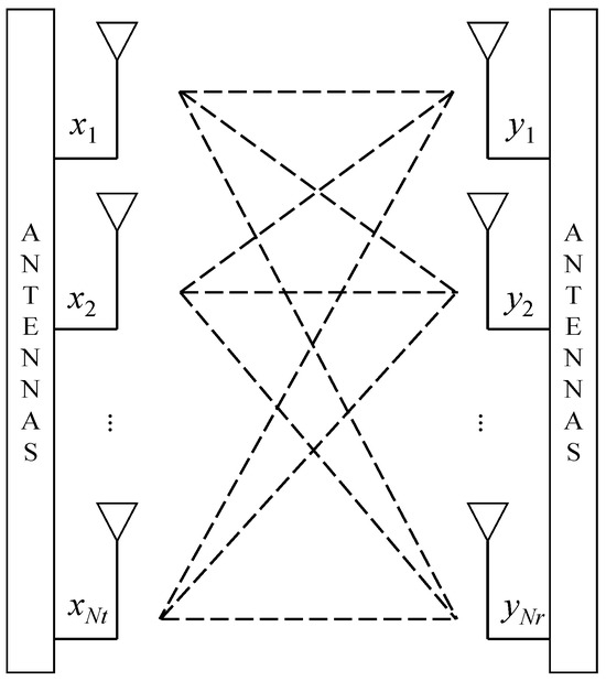
Figure 1.
Diagram of a MIMO system.
The received signal vector (y ) can be written as
In Equation (1), H represents the channel matrix, which contains the coefficients corresponding to the communication links between the transmitter and receiver. The vector expressed as x denotes the modulated or transmitted signals. Finally, w represents the additive white Gaussian noise (AWGN) with zero mean and variance (). These parameters are modeled using complex numbers to characterize a Rayleigh fading channel. However, for easier implementation in programming and coding, we transform the complex-valued model into an equivalent real-valued representation, as presented below.
With the definitions provided in Equation (2), the MIMO channel can be expressed as follows:
In Equation (3), wr has a variance of . Finally, the signal-to-noise ratio (SNR) on a dB scale is defined as follows:
where Es represents the energy per transmit antenna. The total transmit energy is normalized such that NtEs = 1. Additionally, the energy of the signal in Equation (3) is half of Es, denoted as Er = Es/2.
In traditional MIMO detection, the received signal (y) is processed using a filtering approach to mitigate interference and recover the transmitted signal (x). The filtering coefficients are designed based on the channel matrix (H) to suppress interference while minimizing the effects of noise. The general linear detection model is expressed as follows:
where W is the filtering matrix, which varies for zero-forcing (ZF) and minimum mean square error (MMSE) methods. The ZF filter is derived by applying the Moore–Penrose pseudo-inverse of the channel matrix (H):
The MMSE filter incorporates the noise variance () to balance interference suppression and noise minimization:
where I is the identity matrix and (⋅)H represents the Hermitian transpose (conjugate transpose). With the above filters, it is evident that ZF and MMSE are simple methods for detecting the original signal. However, these methods cannot match the performance of maximum likelihood (ML) detection, which is an optimal MIMO detection technique that determines the transmitted signal (x) by exhaustively searching for the candidate that best matches the received signal (y). While ML detection achieves the minimum SER, it is computationally expensive, particularly for large-scale MIMO systems. The ML detection rule finds the x that minimizes the Euclidean distance between the received signal and the expected signal (Hx):
The ML detection method evaluates all possible transmitted symbol combinations and selects the one that minimizes the error. While ML achieves the lowest SER among MIMO detection methods, its computational complexity grows exponentially with the number of transmit antennas (Nt) and the modulation order (M). Specifically, for an Nt-antenna system using M-ary modulation, the complexity is MNt, making ML detection impractical for large-scale MIMO systems.
To overcome this challenge, we propose the use of the VA to reduce complexity while maintaining near-optimal detection performance. Originally designed for the decoding of convolutional codes, the VA is a dynamic programming approach that efficiently finds the most likely transmitted sequence through a trellis-based search, avoiding the need for brute-force enumeration.
2.2. Viterbi Algorithm
In the VA for MIMO detection, the modulation order (M) determines the number of states in the trellis, while the number of receiving antennas (Nr) defines the number of state transitions at each step. This structure allows the algorithm to efficiently explore possible transmitted symbol sequences while reducing computational complexity. The trellis structure of the VA for MIMO detection is illustrated in Figure 2.
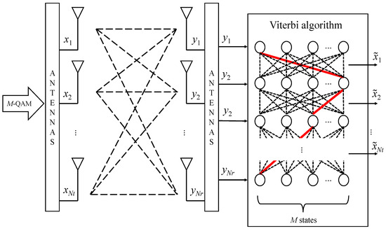
Figure 2.
Viterbi detection for MIMO systems.
In the VA, the trellis diagram represents all possible sequences of transmitted symbols (dashed lines), while the most likely path is estimated and selected (highlighted in red). Each node in the trellis corresponds to a possible state, i.e., a possible transmitted symbol combination. The branch metric is expressed as follows:
Let t = {1, 2, 3, …, Nt} represent the index of the transmitting antenna, corresponding to the t-th time step in the trellis. The branch metric at the t-th time step is denoted as dt. The matrix (Ht) consists of the first t columns of the channel matrix (H). In the symbol vector (xt) elements x(t − 1) represent the symbols from the historic path of the trellis, while the t-th element corresponds to each state in the trellis (e.g., the first state is s1, the second state is s2, and so on).
In each state, the cumulative path metric is calculated as follows:
The path metric () is initialized to zero at t = 0, i.e., . Finally, at t = Nr, the path with the minimum cumulative path metric is selected to detect the signal (x). This ensures that only the most probable sequence of symbols is retained.
2.3. GNN
Unlike other models that process data in matrix or vector formats, GNNs use a graph structure to organize the data. This structure enables GNNs to capture the relationships between elements in the dataset, allowing them to extract features more effectively than other models when working with graph-based data, such as social networks, telecommunications networks, and molecular structures. A graph is composed of nodes (representing entities) and edges (representing the connections between nodes). The primary goal of a GNN is to learn an embedding for each node that incorporates information from its neighboring nodes, reflecting the local graph structure. Once these embeddings are learned, they can be used to generate predictions or outputs related to the graph data. The GNN mechanism is illustrated simply in Figure 3.
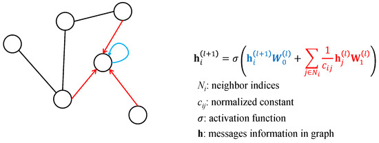
Figure 3.
Mechanism of GNN.
In Figure 3, different colors are used to correspond to the formulas that compute the messages along the arrows. In this paper, we design a GNN structure based on the MIMO configuration. Each antenna is represented as a node, and the connections between antennas are represented as edges in the GNN structure. The transmitting and receiving antennas are paired to form the Tanner graph, as shown in Figure 4. We then apply the GNN calculation mechanism to this Tanner graph.
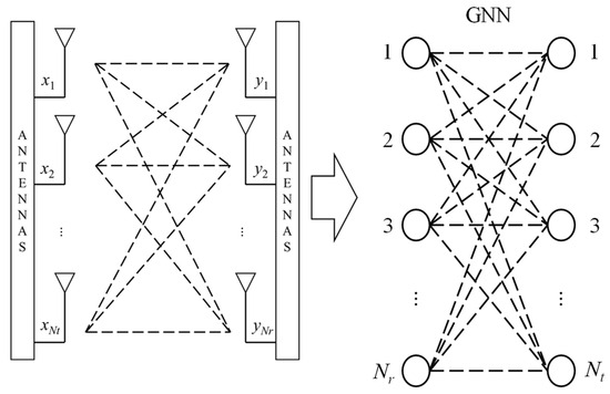
Figure 4.
GNN in MIMO detection.
3. Viterbi-GNN for MIMO Detection
In Figure 5, user data (u) are first modulated into x. The output of the MIMO channel (y) is then processed through Viterbi detection to estimate the initial transmitted signal (). Next, is passed through a GNN to update its values and enhance performance. During training, signals and y are used for message passing within the GNN model. Finally, is updated to and compared with the original x in the loss function. In the testing phase, signals and x are used to evaluate SER performance.
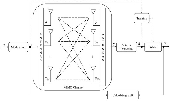
Figure 5.
Diagram of the proposed model.
The output of the VA usually takes hard values, which are not suitable as input for the GNN model. Therefore, in our proposed model, we convert the VA output into soft values. Since the VA output approximates the transmitted signal, we use the following expression to estimate the noise present in the received signal:
From (11), we create the soft output as
The (where 0 1) controls the level of the soft output. As decreases, the output approaches hard values, while as increases, the output becomes softer. However, excessively large values of can introduce noise, leading to a loss of information from the original signal. In this paper, we use = 1 based on [29]. By incorporating soft values in the inner detection process, our proposed model preserves the information of the received signal before providing it to the GNN. As a result, the soft output enhances system performance.
Next, we consider the GNN as a bipartite graph, as shown in Figure 6.
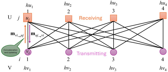
Figure 6.
Message propagations in GNN.
We implement the GNN as follows:
- -
- First, the output of Viterbi detection is input to V nodes by a linear input embedding (hvi = w, where i = 1, 2, …, Nt) and w are trainable coefficients that project the scalar () into a D-dimensional space.
- -
- The message value from V to U is calculated as
- -
- Next, the information on node uj is calculated by the following equation:
- -
- Similarly, from U to V, we can update the message value according to the following expression:
- -
- We calculate the information on node vj as follows:
- -
- The information from U to V and from V to U is updated through N loops. After decoding, the final estimate is = qThvi, where q is another trainable vector that converts hvi, which is D-dimensional, into a scalar ().
The structure of the multilayer perceptron (MLP) in the GNN consists of three layers: an input layer with D = 20 inputs based on [25] (e.g., D-dimensional in GNN structure), a hidden layer with 40 neurons, and an output layer with D outputs. We use the “tanh” function as the activation function in the MLP.
To train the GNN, we use cross-entropy as the loss function, defined as
where p(xi) represents the true probability, which is 1 for an appearing symbol and 0 for a non-appearing symbol. The estimated probability ((x)) is given by the sigmoid function as follows:
We use standard stochastic gradient descent (SGD)-based training with the Adam optimizer. The overall process of the GNN is illustrated in Figure 7.
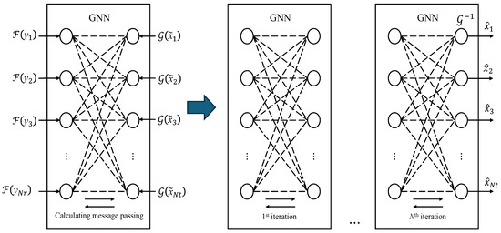
Figure 7.
GNN processing in MIMO detection.
Finally, we compare signal with x to estimate the SER performance.
In our proposed model, the VA is used as a dynamic programming approach to approximate ML detection in MIMO systems. GNNs model the MIMO system as a graph, where nodes represent transmitted symbols and edges capture interference or correlations. GNNs excel in handling high-dimensional, non-linear, and noisy data, and can adapt to varying channel conditions and imperfect channel state information.
A key limitation of GNNs is the lack of initial values for transmitting nodes in the Tanner graph. To address this, we use the VA to generate structured initializations, providing the GNN with a strong starting point. This combination leverages the VA’s sequential consistency and the GNN’s learning ability, resulting in improved detection performance over standalone methods.
4. Results and Discussion
In this section, we configure the simulation to evaluate the model shown in Figure 5. We generate 10,000 samples for each SNR, with each sample containing Nt symbols transmitted through the MIMO channel. The simulation is conducted on a computer equipped with an Intel i5-11400 CPU (2.6 GHz), a GTX 1650 GPU, 16 GB of RAM, and MATLAB 2023a. To collect training data, we generate 10,000 samples with randomly selected SNR values ranging from 9 to 15 dB. The training accuracy curve is shown in Figure 8. In addition, the training parameters are summarized in Table 1.
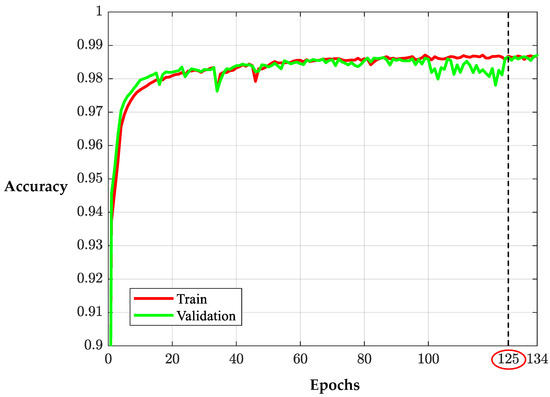
Figure 8.
Learning curves of the GNN model.

Table 1.
The parameters of the training process.
From the learning curves in Figure 8, we observe that after the epoch, the validation curve stabilizes and closely follows the training curve. This behavior indicates that the learning process has converged and reached an optimal performance point. Based on comparative examination conducted around this epoch, we select the epoch as the optimal point for training the parameters of the GNN model.
In the first experiment, we simulate the proposed model with Nr = Nt = 10 and quaternary phase-shift keying (QPSK) modulation (i.e., 4-QAM for a 10 × 10 MIMO system). The results are shown in Figure 9.
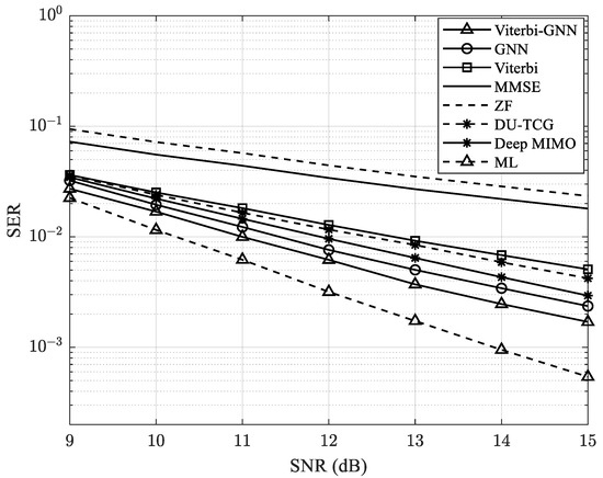
Figure 9.
SER performance of the proposed model.
In Figure 9, our proposed model, Viterbi-GNN, is compared with several baseline methods. The GNN model employs only a GNN-based approach to detect the received signal and recover the original transmitted signal, while Viterbi refers to the model described in [30]. Deep MIMO corresponds to the model introduced in [19], and DU-TCG denotes the deep-unfolded, Tikhonov-regularized conjugate gradient algorithm presented in [8].
Our results demonstrate that the proposed Viterbi-GNN model achieves improved SER performance compared to both traditional and previously proposed deep learning methods. However, it does not surpass the performance of the ML detector, which remains the optimal method for minimizing SER. The ML approach exhaustively searches for the most likely transmitted signal, offering the highest accuracy at the expense of considerable computational complexity.
In the next set of experiments, we increase the number of antennas in the MIMO system to 20 × 20 and 25 × 25 to analyze its impact on system performance. The results, as shown in Figure 10 and Figure 11, demonstrate a clear improvement in SER as the number of antennas increases. This enhancement can be attributed to the improved spatial diversity and signal processing capabilities provided by a larger antenna array, which helps mitigate interference and enhance overall transmission reliability.
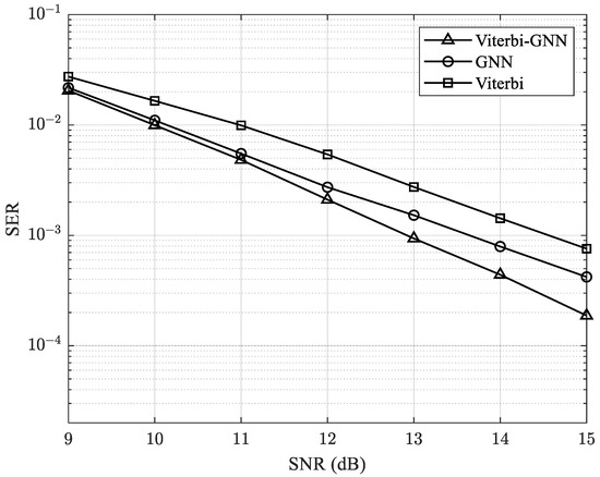
Figure 10.
SER performance of the proposed model with a 20 × 20 MIMO system.
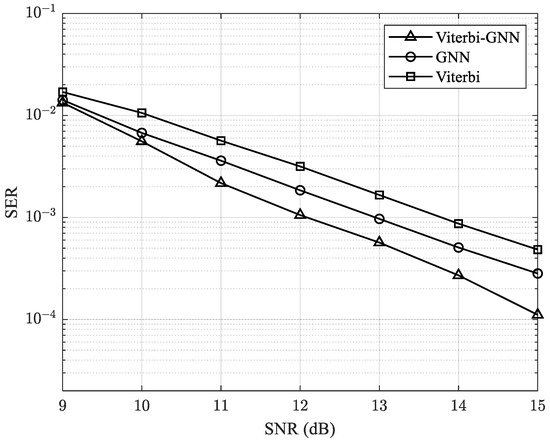
Figure 11.
SER performance of the proposed model with a 25 × 25 MIMO system.
In the next experiment, we configure the MIMO system with a 10 × 10 antenna setup and change the modulation scheme to 16-QAM. The results, presented in Figure 12, provide insights into the impact of modulation on system performance. This experiment helps illustrate how increasing the modulation order affects factors such as the SER and overall transmission efficiency.
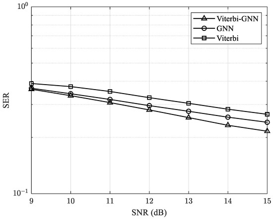
Figure 12.
SER performance of the proposed model with a 16-QAM and 10 × 10 MIMO system.
From Figure 12, it can be observed that as the modulation order (M) increases, the system experiences higher error rates due to several factors. First, the Euclidean distance between symbols decreases, making them more susceptible to noise and interference. Additionally, higher-order modulations are more sensitive to channel fading and distortion, further impacting performance. While these modulations enhance spectral efficiency, this benefit comes at the cost of a higher SER, unless offset by sufficient power and advanced error correction techniques. Nevertheless, our proposed model still outperforms traditional and previous methods, demonstrating improved performance in mitigating these challenges.
Finally, we consider the complexity by using processing time to detect one symbol with 10 × 10 4-QAM antennas. The results are presented in Table 2. We can see the trade-off between SER performance and the complexity of the models.
Table 2.
The processing time for the methods.
5. Conclusions
In this study, we propose a novel Viterbi-GNN detection model for MIMO systems that combines the VA and GNN to enhance detection performance while reducing computational complexity. The VA is used as a pre-processing step to generate an initial estimate of the transmitted signal, which is subsequently refined through a graph-based iterative learning process in the GNN model. By leveraging the Tanner graph structure, our approach effectively captures both the spatial correlations in MIMO channels and the structured dependencies of received signals. Simulation results demonstrate that the Viterbi-GNN detector achieves a lower SER compared to previous MIMO detection methods. However, compared to some previous models, our approach involves a trade-off between detection performance and processing latency.
In future work, we aim to optimize the model structure and reduce computational complexity through techniques such as model compression, pruning, and stochastic computing. We also plan to evaluate the model using real-world 5G/6G testbed datasets to assess its practical applicability. Additionally, we will explore the integration of modulation coding schemes and joint detection–decoding architectures to further enhance system performance and efficiency.
Author Contributions
Conceptualization, T.A.N., X.-T.D., O.-S.S. and J.L.; methodology, T.A.N., X.-T.D., O.-S.S. and J.L.; validation, T.A.N., X.-T.D., O.-S.S. and J.L.; investigation, T.A.N., X.-T.D., O.-S.S. and J.L.; writing—original draft preparation, T.A.N.; writing—review and editing, T.A.N., X.-T.D., O.-S.S. and J.L.; supervision, J.L.; project administration, J.L.; funding acquisition, J.L. All authors have read and agreed to the published version of the manuscript.
Funding
This work was supported by a National Research Foundation of Korea (NRF) grant funded by the Korean government (MSIT) under Grant RS-2023-00208995.
Data Availability Statement
The data presented in this study are available in the article.
Conflicts of Interest
The authors declare no conflicts of interest.
References
- Yang, S.; Hanzo, L. Fifty years of MIMO detection: The road to large-scale MIMOs. IEEE Commun. Surv. Tutor. 2015, 17, 1941–1988. [Google Scholar] [CrossRef]
- Albreem, M.A.; Juntti, M.; Shahabuddin, S. Massive MIMO detection techniques: A survey. IEEE Commun. Surv. Tutor. 2019, 21, 3109–3132. [Google Scholar] [CrossRef]
- Adeva, E.P.; Augustin, T.R.; Fettweis, G.P. Optimizing a pipelined MIMO sphere detector for energy efficiency. In Proceedings of the IEEE International Conference on Wireless Communications & Signal Processing (WCSP), Nanjing, China, 15–17 October 2015; pp. 1–6. [Google Scholar]
- Fukuda, W.; Abiko, T.; Nishimura, T.; Ohgane, T.; Ogawa, Y.; Ohwatari, Y.; Kishiyama, Y. Low-complexity detection based on belief propagation in a massive MIMO system. In Proceedings of the IEEE 77th Vehicular Technology Conference (VTC Spring), Dresden, Germany, 2–5 June 2013; pp. 1–5. [Google Scholar]
- Wu, M.; Yin, B.; Vosoughi, A.; Studer, C.; Cavallaro, J.R.; Dick, C. Approximate matrix inversion for high-throughput data detection in the large-scale MIMO uplink. In Proceedings of the 2013 IEEE International Symposium on Circuits and Systems (ISCAS), Beijing, China, 19–23 May 2013; pp. 2155–2158. [Google Scholar]
- Dai, L.; Gao, X.; Su, X.; Han, S.; Wang, Z. Low-complexity soft output signal detection based on Gauss-Seidel method for uplink multiuser large-scale MIMO systems. IEEE Trans. Veh. Technol. 2015, 64, 4839–4845. [Google Scholar] [CrossRef]
- Yin, B.; Wu, M.; Cavallaro, J.R.; Studer, C. Conjugate gradient-based soft-output detection and precoding in massive MIMO systems. In Proceedings of the 2014 IEEE Global Communications Conference, Austin, TX, USA, 8–12 December 2014; pp. 3696–3701. [Google Scholar]
- Karahan, S.N.; Kalaycıoğlu, A. Deep-unfolded tikhonov-regularized conjugate gradient algorithm for MIMO detection. Electronics 2024, 13, 3945. [Google Scholar] [CrossRef]
- Duong, M.T.; Lee, S.; Hong, M.C. Learning to concurrently brighten and mitigate deterioration in low-light images. IEEE Access 2024, 12, 132891–132903. [Google Scholar] [CrossRef]
- Ho, Q.-T.; Duong, M.-T.; Lee, S.; Hong, M.-C. EHNet: Efficient hybrid network with dual attention for image deblurring. Sensors 2024, 24, 6545. [Google Scholar] [CrossRef] [PubMed]
- Wang, W.; Wu, X.; Yuan, X.; Gao, Z. An experiment-based review of low-light image enhancement methods. IEEE Access 2020, 8, 87884–87917. [Google Scholar] [CrossRef]
- Ahmad, Z.; Khan, A.S.; Shiang, C.W.; Abdullah, J.; Ahmad, F. Network intrusion detection system: A systematic study of machine learning and deep learning approaches. Trans. Emerg. Telecommun. Technol. 2021, 32, e4150. [Google Scholar] [CrossRef]
- Tomar, K.; Bisht, K.; Joshi, K.; Katarya, R. Cyber attack detection in IoT using deep learning techniques. In Proceedings of the 2023 6th International Conference on Information Systems and Computer Networks (ISCON), Mathura, India, 3–4 March 2023; pp. 1–6. [Google Scholar]
- Nguyen, T.A.; Lee, J. Using long short-term memory to estimate the 2-D interference of bit-patterned media recording systems. IEEE Trans. Magn. 2024, 60, 1–5. [Google Scholar]
- Sayyafan, A.; Aboutaleb, A.; Belzer, B.J.; Sivakumar, K.; Aguilar, A.; Pinkham, C.A.; Chan, K.S.; James, A. Deep neural network media noise predictor turbo-detection system for 1-D and 2-D high-density magnetic recording. IEEE Trans. Magn. 2021, 57, 1–13. [Google Scholar] [CrossRef]
- Dang, X.T.; Nguyen, H.V.; Shin, O.S. Physical layer security for IRS-UAV-assisted cell-free massive MIMO systems. IEEE Access 2024, 12, 89520–89537. [Google Scholar] [CrossRef]
- Dai, L.; Jiao, R.; Adachi, F.; Poor, H.V.; Hanzo, L. Deep learning for wireless communications: An emerging interdisciplinary paradigm. IEEE Wirel. Commun. 2020, 27, 133–139. [Google Scholar] [CrossRef]
- Hu, Q.; Gao, F.; Zhang, H.; Li, G.Y.; Xu, Z. Understanding deep MIMO detection. IEEE Trans. Wirel. Commun. 2023, 22, 9626–9639. [Google Scholar] [CrossRef]
- He, H.; Wen, C.K.; Jin, S.; Li, G.Y. A model-driven deep learning network for MIMO detection. In Proceedings of the 2018 IEEE Global Conference on Signal and Information Processing (GlobalSIP), Anaheim, CA, USA, 26–29 November 2018; pp. 584–588. [Google Scholar]
- Un, M.W.; Shao, M.; Ma, W.K.; Ching, P.C. Deep MIMO detection using ADMM unfolding. In Proceedings of the 2019 IEEE Data Science Workshop (DSW), Toronto, ON, Canada, 2–5 June 2019; pp. 333–337. [Google Scholar]
- Ge, Y.; Tan, X.; Ji, Z.; Zhang, Z.; You, X.; Zhang, C. Improving approximate expectation propagation massive MIMO detector with deep learning. IEEE Wirel. Commun. Lett. 2021, 10, 2145–2149. [Google Scholar] [CrossRef]
- Baek, M.S.; Kwak, S.; Jung, J.Y.; Kim, H.M.; Choi, D.J. Implementation methodologies of deep learning-based signal detection for conventional MIMO transmitters. IEEE Trans. Broadcast. 2019, 65, 636–642. [Google Scholar] [CrossRef]
- Tran, D.-H.; Park, M. FN-GNN: A novel graph embedding approach for enhancing graph neural networks in network intrusion detection systems. Appl. Sci. 2024, 14, 6932. [Google Scholar] [CrossRef]
- Le, H.-D.; Park, M. Enhancing multi-class attack detection in graph neural network through feature rearrangement. Electronics 2024, 13, 2404. [Google Scholar] [CrossRef]
- Cammerer, S.; Hoydis, J.; Aoudia, F.A.; Keller, A. Graph neural networks for channel decoding. In Proceedings of the 2022 IEEE Globecom Workshops (GC Wkshps), Rio de Janeiro, Brazil, 4–8 December 2022; pp. 486–491. [Google Scholar]
- Shen, Y.; Zhang, J.; Song, S.H.; Letaief, K.B. Graph neural networks for wireless communications: From theory to practice. IEEE Trans. Wirel. Commun. 2023, 22, 3554–3569. [Google Scholar] [CrossRef]
- Nguyen, T.A.; Lee, J. Graph neural network (GNN) for joint detection–decoder MAP–LDPC in bit-patterned media recording systems. Electronics 2024, 13, 4811. [Google Scholar] [CrossRef]
- Xu, T.; Tan, X.; Zhang, Z.; You, X.; Zhang, C. MIMO detection based on graph neural network with belief propagation. In Proceedings of the IEEE 2023 International Conference on Wireless Communications and Signal Processing (WCSP), Hangzhou, China, 2–4 November 2023; pp. 1095–1100. [Google Scholar]
- Nguyen, T.A.; Lee, J. Serial detection with neural network-based noise prediction for bit-patterned media recording systems. Appl. Sci. 2021, 11, 4387. [Google Scholar] [CrossRef]
- Lee, J.; Park, S.-C. MIMO detector based on Viterbi algorithm. In Proceedings of the 2007 IEEE Workshop on Signal Processing Systems, Shanghai, China, 17–19 October 2007; pp. 111–115. [Google Scholar]
Disclaimer/Publisher’s Note: The statements, opinions and data contained in all publications are solely those of the individual author(s) and contributor(s) and not of MDPI and/or the editor(s). MDPI and/or the editor(s) disclaim responsibility for any injury to people or property resulting from any ideas, methods, instructions or products referred to in the content. |
© 2025 by the authors. Licensee MDPI, Basel, Switzerland. This article is an open access article distributed under the terms and conditions of the Creative Commons Attribution (CC BY) license (https://creativecommons.org/licenses/by/4.0/).