Joint Optimization of Model Partitioning and Resource Allocation for Multi-Exit DNNs in Edge-Device Collaboration

Abstract

The increasing complexity and computational demands of deep neural networks (DNNs) pose significant challenges and deployment on resource-constrained devices due to substantial latency and considerable energy consumption. Multi-exit DNNs have emerged as a promising solution, enabling simple tasks to exit early at intermediate network layers, thereby reducing inference latency and improving efficiency. However, relying solely on the computational capacity of end devices is often insufficient to meet performance requirements. Edge computing, by offloading part of the model’s computation to edge servers, has become a key solution to address this issue. Despite the potential of multi-exit DNNs in edge computing environments, two major challenges remain: model partitioning and resource allocation on edge servers. Existing research often focuses on model partitioning strategies or resource allocation strategies in isolation, neglecting the mutual optimization between the two. Moreover, energy consumption, a critical performance metric, is frequently overlooked in the optimization process. To address these issues, this paper proposes a joint optimization framework for model partitioning and resource allocation, integrating multi-exit DNNs and incorporating a deep reinforcement learning (DRL)-based optimization algorithm. Experimental results demonstrate that the proposed method significantly reduces inference costs and enhances system performance.

1. Introduction

With the rapid advancement of DNNs [1], significant breakthroughs have been achieved in fields such as computer vision and natural language processing. However, as model performance improves, the increasing depth and complexity of DNNs also lead to a notable rise in inference latency and energy consumption. This issue is particularly critical for latency- and energy-sensitive tasks, such as real-time monitoring and online interactive systems. Consequently, how to effectively reduce inference latency and energy consumption while maintaining model performance has become a crucial research topic in the field of DNNs.

In response to this challenge, multi-exit DNNs [2] have emerged as an innovative architectural design, providing a novel solution to mitigate the high computational cost and energy consumption of DNNs. By embedding multiple early exits in the intermediate layers of the network, multi-exit DNNs allow input samples to terminate inference prematurely once predefined exit conditions are met. This approach significantly reduces computational overhead and improves inference efficiency without compromising model accuracy. Such architecture is particularly suitable for scenarios with unevenly distributed task complexities, such as object recognition, video analysis, and real-time monitoring, demonstrating considerable flexibility and practicality.

Nevertheless, relying solely on the computational capacity of end devices is insufficient to meet the increasing computational demands. With the advent of edge computing, edge servers can provide powerful computational support to end devices, enabling efficient collaborative computing. End-edge collaborative inference [3] has thus emerged as a promising solution. By partitioning the multi-exit DNN into shallow and deep layers, where the shallow layers are deployed on end devices and the deep layers on edge servers, this collaborative inference framework can significantly reduce the computational burden and energy consumption of end devices while maintaining inference accuracy. Moreover, this approach effectively addresses the challenges of real-time requirements and resource-constrained environments.

Despite the promising performance advantages of multi-exit DNNs in edge computing environments, their practical deployment faces two key challenges: the model partitioning problem and the edge server resource allocation problem. First, due to differences in network structures, the optimal partitioning strategy varies significantly across different multi-exit DNNs. Additionally, heterogeneous end devices face distinct task difficulties, resulting in varying demands for edge server computational resources. Improper resource allocation may lead to resource skewness, which can degrade overall inference performance. Furthermore, the optimal model partitioning decision and resource allocation strategy are interdependent. Specifically, the partitioning position directly affects data transmission volume, edge server computation load, and end device energy consumption. Conversely, adjustments in resource allocation strategy can significantly impact inference latency, overall performance, and end device energy consumption. Consequently, optimizing a single aspect alone is insufficient to achieve optimal results in minimizing latency and energy consumption.

However, existing studies often focus on optimizing model partitioning strategies while overlooking the critical impact of resource allocation on performance. Conversely, some studies focus on optimizing resource allocation based on fixed model partitioning schemes but fail to dynamically adjust model partitioning strategies. Although a few studies have attempted joint optimization of both aspects, they often neglect the crucial factor of energy consumption.

To address these issues, this paper proposes a collaborative computing framework based on multi-exit DNNs, aiming to jointly optimize the model partitioning and resource allocation decisions. This framework effectively reduces inference latency and energy consumption while ensuring inference accuracy constraints.

The main contributions of this paper are as follows:

• We establish a joint optimization model for model partitioning and resource allocation in end–edge collaborative computing based on multi-exit DNNs.
• We design an efficient algorithm to determine the optimal partitioning points and resource allocation ratios.
• We conduct experiments to verify the proposed method’s superiority in terms of latency and energy consumption.

This paper is structured as follows: Section 2 reviews related work on end–edge collaborative inference with multi-exit DNNs. Section 3 describes the system model, detailing inference latency, energy consumption, and the corresponding optimization problem. Section 4 presents our proposed joint optimization algorithm for model partitioning and resource allocation under multi-objective constraints. Section 5 evaluates the method’s effectiveness via simulations, analyzing inference latency, energy consumption, and overall performance. Section 6 concludes the paper.

2. Related Work

Recent advancements in collaborative inference between end devices and edge servers using multi-exit DNNs have effectively harnessed the benefits of both. This approach enables early task exits while maintaining accuracy, thereby saving energy, and reduces the computational burden on local devices by fully utilizing both local and edge server resources. As a result, inference efficiency is enhanced, while latency and energy consumption are significantly reduced. However, several limitations persist in existing research. Some studies focus exclusively on model partitioning or resource allocation, overlooking their mutual optimization. Additionally, some studies optimize inference latency as the primary objective, without fully considering energy consumption, a key performance metric. Furthermore, some studies rely on fixed exit configurations for optimization, which fails to dynamically adjust the exit points based on task complexity, leading to poor adaptability.

First, existing studies have extensively explored model partitioning strategies to improve inference performance in collaborative inference systems. However, these studies largely overlook the optimization of resource allocation. For instance, some studies focus on identifying optimal partition points to balance latency, energy consumption, and model accuracy in computation offloading and task scheduling [4]. Others have proposed strategies that integrate early exit mechanisms to enhance inference efficiency [5] or introduced reinforcement learning-based mechanisms that dynamically adjust exit points in multi-access edge computing networks to maximize throughput and accuracy [6]. Additionally, some works have explored joint optimization frameworks that combine model partitioning with confidence threshold tuning [7] or determine the optimal DNN depth for edge computing based on accuracy, computational efficiency, and communication costs [8]. To enhance adaptability under dynamic conditions, some studies introduce novel schedulers that jointly optimize early exit strategies and CNN partitioning [9,10], while others propose dynamic DNN partitioning schemes that adjust to network conditions at the computational layer granularity [11]. Furthermore, some approaches select model partition points based on device load, cloud load, and network conditions [12]. Although these methods have achieved significant improvements in inference efficiency, they predominantly focus on model partitioning while neglecting the critical role of resource allocation in optimizing overall system performance. Inefficient resource allocation may lead to resource imbalance, further constraining system performance improvements.

Second, some studies have optimized resource allocation based on predetermined model partitioning schemes, neglecting the dynamic adjustment of partitioning strategies. For example, Reference [13] explored the joint allocation of communication and computational resources to meet heterogeneous user requirements for accuracy and latency. Reference [14] proposed an end-to-end cooperative computing system based on multi-exit networks, which dynamically allocates computation between front-end camera sensors and back-end mobile edge computing servers to minimize inference time under varying channel conditions.

Moreover, a considerable number of studies overlook energy consumption as a critical performance metric. While the study in [15] jointly optimizes model partitioning and resource allocation, it focuses solely on minimizing latency. Some studies [5,7,16,17] aim to optimize latency and accuracy, while others [11,14] prioritize latency reduction under accuracy constraints or focus on maximizing throughput [13,18], neglecting energy consumption in the process. In practical applications, energy consumption is a crucial factor in evaluating system performance, particularly for resource-constrained mobile and IoT devices. Ignoring energy optimization may lead to reduced battery life, ultimately compromising the system’s sustainability.

Some studies on model partitioning are based on the optimization of fixed-structure multi-exit neural networks, failing to fully exploit the flexibility of multi-exit architectures. References [4,18] conduct their research based on the multi-exit DNN structure defined by the BranchyNet framework [2], overlooking the more flexible exit placement strategies that adapt to the distribution of task complexity, which have gained popularity in recent research. The fixed exit placement strategy is unable to accommodate dynamic variations in task complexity, potentially resulting in wasted computational resources or degraded performance.

In summary, existing research exhibits limitations in model partitioning, resource allocation, and the trade-off between latency and energy consumption. Consequently, this study aims to address these challenges by proposing a more flexible and effective model partitioning and resource allocation scheme based on multi-exit DNNs, targeting multi-objective optimization with respect to latency, accuracy, and energy consumption.

3. System Model and Optimization Problem

3.1. System Model

This study focuses on the scenario of collaborative inference between heterogeneous end devices and edge computing, involving multiple heterogeneous end devices and a single edge server. We denote the set of end devices by $i=\{0,1,2,\dots ,N\}$, where N is the total number of end devices.

A multi-exit DNN consists of a backbone network and several exit branches. The backbone network typically includes convolutional layers, pooling layers, ReLU activation functions, fully connected layers, and softmax layers, while the exit branches primarily consist of classifiers. For simplification, the backbone network is abstracted as several logical layers and a final exit. Specifically, the fully connected layer and softmax layer at the model’s end are combined into the final output layer, while each convolutional layer and its subsequent pooling layers and ReLU activation functions, up to the next convolutional layer or before the final output layer, are defined as a logical layer. Exit branches are inserted after the logical layers, allowing tasks that meet the exit conditions to exit early.

When deploying a pre-trained multi-exit DNN on end devices, to accommodate the diversity in input sample complexity processed by different end devices, the structure of the multi-exit DNN deployed on each end device may vary. As shown in Figure 1, in the collaborative inference scenario between end devices and edge servers, the multi-exit DNN with $L_i$ layers of logical layers is divided into two parts: shallow layers (from layer 0 to layer $h_i$, where $h_i\in \{0,1,2,\dots ,L_i\}$) are deployed on the end device, and deep layers (from layer $h_i+1$ to layer $L_i$, where $h_i\in \{0,1,2,\dots ,L_i\}$) are offloaded to the edge server. To measure the computational overhead of model inference, we define $C_{i,j}^{\mathrm{logic}}$ and $C_{i,j}^{\mathrm{exit}}$ as the floating point operations (FLOPs) at logical layer j and at the corresponding exit, respectively. $W_i^{h_i}$ represents the amount of intermediate data generated by the multi-exit DNN on end device i at logical layer $h_i$, i.e., the size of the data transmitted from logical layer $h_i$ to logical layer $h_i+1$.

Once a task enters inference on the end device, if it satisfies the early exit conditions, it can exit early at the corresponding exit branch. For tasks that do not exit early on the end device, the intermediate results generated during inference on the end device will be offloaded to the edge server for further computation, until the task satisfies the exit condition or reaches the final output.

For image tasks, the task sequentially explores the exit branches to identify the optimal exit, which is the first exit branch where the maximum softmax output exceeds a predefined threshold. At each exit, the task compares the maximum value of the softmax output with the threshold, and if it reaches the predefined threshold, the task exits at that branch; otherwise, it continues passing deeper into the network until an exit meeting the condition is found or the final output is reached. For video tasks, we adopt the efficient exit rule proposed in reference [19], utilizing the strong correlation between adjacent video frames to predict the optimal exit for the current frame. Specifically, if the complexity of the current frame exceeds that of the previous frame, some exits are skipped, and the task begins attempting to exit from the exit used in the previous frame’s task to reduce redundant computation; otherwise, the task attempts exits sequentially, similar to image tasks.

Regardless of the exit rule used, the probability of performing computations at each logical layer and exit can be recorded, denoted by $P_{i,j}^{\mathrm{logic}},i\in \{1,2,\dots ,N\},j\in \{1,2,\dots ,L_i\}$ and $P_{i,j}^{\mathrm{exit}},i\in \{1,2,\dots ,N\},j\in \{1,2,\dots ,L_i\}$, respectively. If a logical layer j does not have an exit, then $P_{i,j}^{\mathrm{exit}}=0$.

To characterize the inference latency and energy consumption under different model partitioning schemes $H=\{h_1,h_2,\dots ,h_i,\dots ,h_N\}$ and resource allocation strategies $Y=\{y_1,y_2,\dots ,y_i,\dots ,y_N\}$, we further introduce relevant variables, and the mathematical symbols and their specific meanings are listed in

Table 1. Symbols and definitions.

Symbol	Definition
$L_i$	The number of logical layers in the complete multi-exit DNN deployed on end device i.
$C_{i,j}^{\mathrm{exit}}$	The FLOPs required to infer a task at exit branch j of the multi-exit DNN deployed on end device i.
$C_{i,j}^{\mathrm{logic}}$	The FLOPs required to infer a task at logical layer j of the multi-exit DNN deployed on end device i.
$P_{i,j}^{\mathrm{logic}}$	The probability that a task produces computation at logical layer j.
$P_{i,j}^{\mathrm{exit}}$	The probability that a task produces computation at exit branch j.
$R_i^{\mathrm{device}}$	The computational capability of end device i.
$R_{\mathrm{edge}}$	The computational capability of the edge server.
${\mathrm{pow}}_i^{\mathrm{device}}$	The power consumption of end device i.
${\mathrm{pow}}_i^{\mathrm{trans}}$	The transmission power from end device i to the edge server.
B	The bandwidth size for data transmission.
$W_i^{h_i}$	The size of intermediate data passed between layers.
$y_i$	The proportion of resources allocated by the edge server for offloading tasks from end device i.
$h_i$	The splitting point of the DNN on end device i.
${\mathrm{COS}\mathrm{T}}_i\left(YH\right)$	The overall cost function for end device i.

. Subsequently, we model the expected inference cost of the task, which consists of both latency and energy consumption. A schematic illustration of the cost components is provided in Figure 2. The modeling methods for latency and energy consumption are presented next.

3.2. Latency Model

The expected inference latency of a task comprises three components: the expected local inference latency on end device i, denoted as $T_i^{\mathrm{device}}\left(YH\right)$; the expected transmission latency for transferring intermediate data from end device i to the edge server, denoted as $T_i^{\mathrm{trans}}\left(YH\right)$; and the expected inference latency at the edge server, denoted as $T_i^{\mathrm{edge}}\left(YH\right)$. The detailed latency computations for each component are described below.

3.2.1. Expected Local Inference Latency on End Device i

The expected local inference latency on end device i is defined as the total FLOPs required to process a task within the shallow layers (from layer 0 to layer $h_i$) of the multi-exit DNN deployed on the device, divided by the computational capability of the device, as follows:

$$T_i^{\mathrm{device}}\left(YH\right)={\displaystyle \frac{{\sum }_{j=1}^{h_i}\left(P_{i,j}^{\mathrm{logic}}·C_{i,j}^{\mathrm{logic}}+P_{i,j}^{\mathrm{exit}}·C_{i,j}^{\mathrm{exit}}\right)}{R_i^{\mathrm{device}}}}.l$$

(1)

Here, $R_i^{\mathrm{device}}$ represents the computational capability of end device i, while $C_{i,j}^{\mathrm{logic}}$ and $C_{i,j}^{\mathrm{exit}}$ denote the FLOPs required to infer a task at logical layer j and at the exit corresponding to logical layer j, respectively. $P_{i,j}^{\mathrm{logic}}$ and $P_{i,j}^{\mathrm{exit}}$ represent the probabilities of performing computations at logical layer j and at the exit corresponding to logical layer j in the multi-exit DNN of device i, respectively.

3.2.2. Expected Transmission Latency

The expected transmission latency between end device i and the edge server can be expressed as the product of the intermediate data size output at partition layer $h_i$, and the probability of the task being offloaded to the edge server for further inference, divided by the available bandwidth. Specifically, it is given by

$$T_i^{\mathrm{trans}}\left(YH\right)={\displaystyle \frac{W_i^{h_i}·P_{i,h_i+1}^{\mathrm{logic}}}{B}},$$

(2)

where B denotes the network bandwidth, $W_i^{h_i}$ represents the size of the intermediate data transferred from logical layer $h_i$ to layer $h_i+1$ within the multi-exit DNN on device i, and $P_{i,h_i+1}^{\mathrm{logic}}$ is the probability that the task is offloaded to the edge server for continued inference.

3.2.3. Expected Inference Latency at the Edge Server

The expected inference latency at the edge server is computed as the total FLOPs required for processing a task within the deeper layers (from logical layer $h_i+1$ to $L_i$) of the multi-exit DNN, divided by the computational resources allocated to end device i at the edge server, as follows:

$$T_i^{\mathrm{edge}}\left(YH\right)={\displaystyle \frac{{\sum }_{j=h_i+1}^{L_i}\left(P_{i,j}^{\mathrm{logic}}{C}_{i,j}^{\mathrm{logic}}+P_{i,j}^{\mathrm{exit}}{C}_{i,j}^{\mathrm{exit}}\right)}{y_i{R}_{\mathrm{edge}}}},$$

(3)

where $R_{\mathrm{edge}}$ represents the computational capability of the edge server, and $y_i\in [0,1]$ denotes the proportion of edge server resources allocated to end device i.

3.2.4. Total Expected Inference Latency

The total inference latency of a task, from input at end device i to completion of inference, is the sum of the three aforementioned latency components, as follows:

$$T_i\left(YH\right)=T_i^{\mathrm{device}}\left(YH\right)+T_i^{\mathrm{trans}}\left(YH\right)+T_i^{\mathrm{edge}}\left(YH\right).$$

(4)

3.3. Energy Consumption Model

In the end-edge collaborative computing framework, inference tasks’ energy consumption on the edge server is negligible due to its stable and uninterrupted power supply from the electrical grid [3]. Consequently, the expected inference energy consumption is primarily composed of the local inference energy consumption on end device i, denoted as ${\mathrm{ene}}_i^{\mathrm{device}}$, and the network transmission energy consumption, denoted as ${\mathrm{ene}}_i^{\mathrm{trans}}$. The detailed energy consumption calculations for each component are described below.

3.3.1. Expected Local Inference Energy Consumption on End Device i

The local inference energy consumption on device i is given by the product of its power consumption ${\mathrm{pow}}_i^{\mathrm{device}}$ and the expected local inference latency $T_i^{\mathrm{device}}\left(YH\right)$, as follows:

$${\mathrm{ene}}_i^{\mathrm{device}}={\mathrm{pow}}_i^{\mathrm{device}}·T_i^{\mathrm{device}}\left(YH\right),$$

(5)

where ${\mathrm{pow}}_i^{\mathrm{device}}$ represents the power consumption of end device i.

3.3.2. Expected Network Transmission Energy Consumption on End Device i

The network transmission energy consumption for end device i equals the product of its transmission power ${\mathrm{pow}}_i^{\mathrm{trans}}$ and the expected transmission latency $T_i^{\mathrm{trans}}\left(YH\right)$, as follows:

$${\mathrm{ene}}_i^{\mathrm{trans}}={\mathrm{pow}}_i^{\mathrm{trans}}·T_i^{\mathrm{trans}}\left(YH\right),$$

(6)

where ${\mathrm{pow}}_i^{\mathrm{trans}}$ denotes the power consumption of end device i during the transmission of the task to the edge server.

3.3.3. Total Expected Inference Energy Consumption

The expected total energy consumption from the input of the task on end device i to the completion of inference can be expressed as the sum of the expected inference energy consumption on end device i and the expected network transmission energy consumption, as follows:

$${\mathrm{ene}}_i\left(YH\right)={\mathrm{ene}}_i^{\mathrm{device}}+{\mathrm{ene}}_i^{\mathrm{trans}}.$$

(7)

3.4. Optimization Problem

The overall cost of inference for end device i, denoted as ${\mathrm{COS}\mathrm{T}}_i\left(YH\right)$, consists of two components: the expected inference latency and the expected energy consumption, which can be expressed as follows:

$${\mathrm{COS}\mathrm{T}}_i\left(YH\right)=\mu ·T_i\left(YH\right)+\nu ·{\mathrm{ene}}_i\left(YH\right),$$

(8)

where $\mu$ and $\nu$ are weight coefficients that balance the relative importance of latency and energy consumption in the overall inference cost.

Our objective is to effectively minimize the average inference cost across all end devices by jointly optimizing the partitioning strategy $H=\{h_1,h_2,\dots ,h_i,\dots ,h_N\}$ and the resource allocation ratio $Y=\{y_1,y_2,\dots ,y_i,\dots ,y_N\}$, which can be formulated as the following optimization problem:

$$\mathrm{P}1:min{\displaystyle \frac{{\sum }_{i=1}^N{\mathrm{COS}\mathrm{T}}_i\left(YH\right)}{N}}.$$

(9)

$$\begin{array}{cc}\hfill \mathrm{s}.\mathrm{t}.\sum _{i=1}^N{y}_i& =1,y_i\in [0,1]\hfill \end{array}$$

(9a)

$$\begin{array}{cc}\hfill h_i& \in \{0,1,2,\dots ,L_i\},\forall i\in N\hfill \end{array}$$

(9b)

4. Algorithm Design

According to the system model, the partition layer $h_i$ is an integer, while the resource allocation decision $y_i$ falls within the range of $[0,1]$, making this optimization problem a mixed-integer programming problem. With the introduction of the early exit mechanism, the execution path of tasks exhibits significant diversity. Specifically, the probability $P_{i,j}^{\mathrm{logic}}$ of a task reaching logical layer j becomes discontinuous due to the introduction of exit branches, thereby transforming the original problem into a non-convex optimization problem. This makes it challenging to directly apply traditional mathematical optimization methods to solve the problem.

To tackle this challenge, we propose a DRL-based joint optimization algorithm for multi-exit DNN partitioning and resource allocation, aiming to minimize inference latency and energy consumption. The algorithm adopts the Proximal Policy Optimization (PPO) framework, a policy optimization-based reinforcement learning approach, and employs a dual neural network structure (Actor–Critic) to solve optimization problem P1.

PPO is a reinforcement learning algorithm that optimizes policies by clipping updates to ensure stability while accelerating convergence. In this problem, PPO utilizes an Actor–Critic architecture, where

• The Actor network generates the optimal actions under the current system state (i.e., model partitioning and resource allocation decisions); and
• The Critic network evaluates the value of the current state and guides policy improvement.

Below, we provide a detailed explanation of the algorithm design and implementation.

4.1. Mapping the Optimization Problem to DRL

The objective of optimization problem $P1$ is to minimize the average inference cost ${\mathrm{COS}\mathrm{T}}_i\left(YH\right)$ for all end devices, where the cost consists of both latency and energy consumption. To transform this problem into a DRL-compatible format, we define the following mapping function:

$$\Pi :\left\{P_{i,j}^{\mathrm{logic}},P_{i,j}^{\mathrm{exit}},C_{i,j}^{\mathrm{logic}},C_{i,j}^{\mathrm{exit}},R_i^{\mathrm{device}},R_{\mathrm{edge}},{\mathrm{pow}}_i^{\mathrm{device}},{\mathrm{pow}}_i^{\mathrm{trans}},B\mid j\in L_i,i\in N\right\}\to a^{*},$$

(10)

where $\Pi$ represents the mapping from the system state to the optimal action $a^{*}$.

4.2. State Space

The state space comprehensively captures all relevant system information, including task characteristics, resource availability, and network conditions. The system state at time t is defined as

$$\begin{array}{cc}\hfill s_i\left(t\right)=& \left\{P_{i,j}^{\mathrm{logic}},P_{i,j}^{\mathrm{exit}},C_{i,j}^{\mathrm{logic}},C_{i,j}^{\mathrm{exit}},R_i^{\mathrm{device}},R_{\mathrm{edge}},{\mathrm{pow}}_i^{\mathrm{device}},{\mathrm{pow}}_i^{\mathrm{trans}},B,\right.\hfill \\ \hfill & T_i^{\mathrm{device}}(t-k),T_i^{\mathrm{trans}}(t-k),T_i^{\mathrm{edge}}(t-k),T_i(t-k),{\mathrm{ene}}_i^{\mathrm{device}}(t-k),\hfill \\ \hfill & \left.{\mathrm{ene}}_i^{\mathrm{trans}}(t-k),{\mathrm{ene}}_i(t-k)\mid j\in L_i,i\in N,k<t\right\}\hfill \end{array}$$

(11)

Here, t denotes the current time step, and k represents historical time steps. We retain the latency and energy consumption data from the most recent $t-k$ time steps to enable the agent to learn from temporal trends.

4.3. Action Space

To ensure that model partitioning decision $h_i\left(t\right)$ and resource allocation decision $y_i\left(t\right)$ adhere to their respective constraints, we preprocess both actions.

Model Partitioning Decision: Since $h_i\left(t\right)$ is a discrete variable within $\{0,1,2,\dots ,L_i\}$, directly using it as an action output would result in an excessively large discrete action space. Instead, we apply rounding and mapping, as follows:

$$h_i\left(t\right)=\mathrm{round}\left(L_i·\sigma \left({\tilde{h}}_i\left(t\right)\right)\right),$$

(12)

where ${\tilde{h}}_i\left(t\right)$ is the continuous output from the policy network, and the sigmoid function $\sigma$ restricts the output to the interval $[0,1]$.

Resource Allocation Decision: Since $y_i\left(t\right)$ is a continuous variable in $[0,1]$, we use sigmoid normalization to satisfy the constraint ${\sum }_{i=1}^N{y}_i=1$, as follows:

$$y_i\left(t\right)={\displaystyle \frac{\sigma \left({\tilde{y}}_i\left(t\right)\right)}{{\sum }_{j=1}^N{y}_j\left(t\right)}},$$

(13)

where ${\tilde{y}}_i\left(t\right)$ is the continuous output from the policy network.

Thus, the action $a_i\left(t\right)$ for end device i is defined as

$$a_i\left(t\right)=[y_i\left(t\right),h_i\left(t\right)].$$

(14)

4.4. Reward Function Design

The reward function $g\left(t\right)$ is constructed to capture the relative improvement in inference performance over time. Since the primary optimization objectives are to reduce inference latency and energy consumption, the reward is defined based on the temporal change in the average inference cost, formulated as follows:

$$g\left(t\right)=-\alpha ·\left({\mathrm{COS}\mathrm{T}}_{\mathrm{ratio}}\left(t\right)-1\right),$$

(15)

where $\alpha >0$ is a coefficient that adjusts the size of the reward, and ${\mathrm{COS}\mathrm{T}}_{\mathrm{ratio}}\left(t\right)$ represents the ratio of the average inference cost at time step t to the average inference cost at the previous time step $t-1$, expressed as

$${\mathrm{COS}\mathrm{T}}_{\mathrm{ratio}}\left(t\right)={\displaystyle \frac{\mathrm{avg}\_\mathrm{COST}(t)}{\mathrm{avg}\_\mathrm{COST}(t-1)}},$$

(16)

4.5. Policy Optimization Using PPO

PPO is a policy gradient-based optimization method that maximizes an objective function to improve the policy iteratively. The core idea is clipping policy updates to avoid instability. The PPO loss function is defined as

$$L^{CLIP}\left(\theta \right)={\widehat{E}}_t\left[min\left(r_t\left(\theta \right){\widehat{A}}_t,\mathrm{clip}\left(r_t\left(\theta \right),1-ϵ,1+ϵ\right){\widehat{A}}_t\right)\right],$$

(17)

where

$$r_t\left(\theta \right)={\displaystyle \frac{Y{H}_{\theta }\left(a\left(t\right)\right|s\left(t\right))}{Y{H}_{\mathrm{old}}\left(a\left(t\right)\right|s\left(t\right))}}$$

(18)

represents the probability ratio between the current policy and the previous policy. ${\widehat{A}}_t$ denotes the advantage function, which quantifies the relative benefit of the current action compared with the average action. To mitigate variance during training, this study employs Generalized Advantage Estimation (GAE) to estimate the advantage function. The function $\mathrm{clip}(·)$ serves as a clipping mechanism to constrain the range of $r_t\left(\theta \right)$, thereby preventing excessively large updates to the policy. The parameter $ϵ$ represents the clipping threshold, which controls the extent of policy updates.

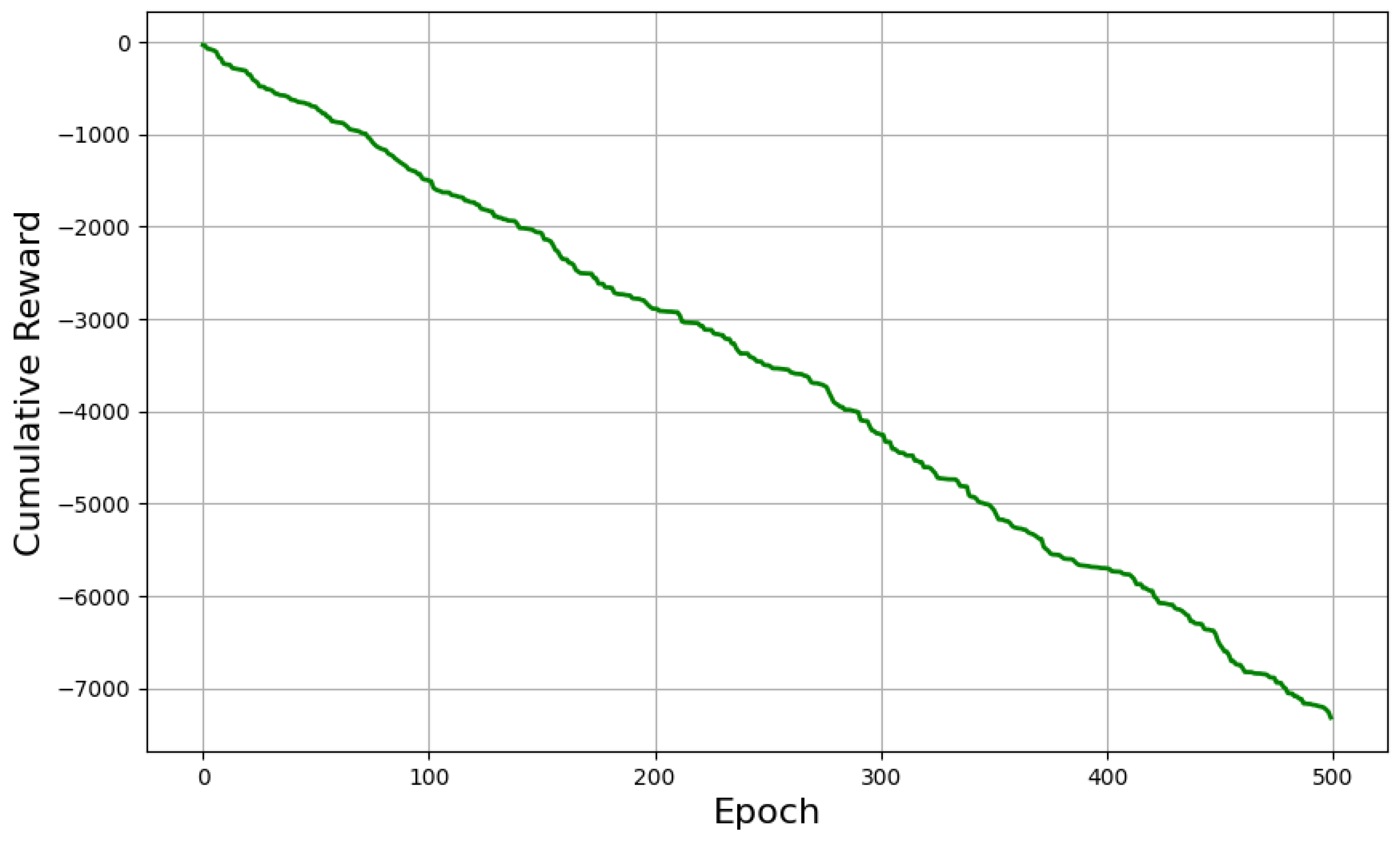
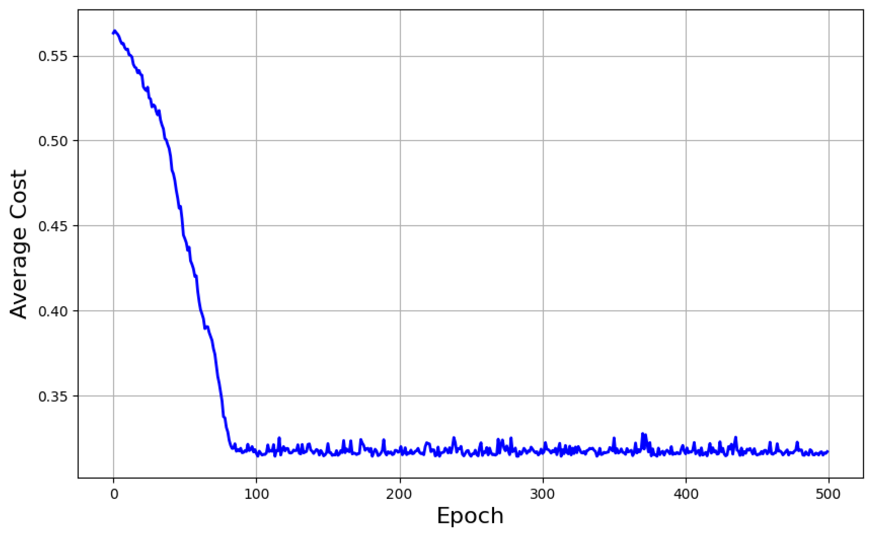
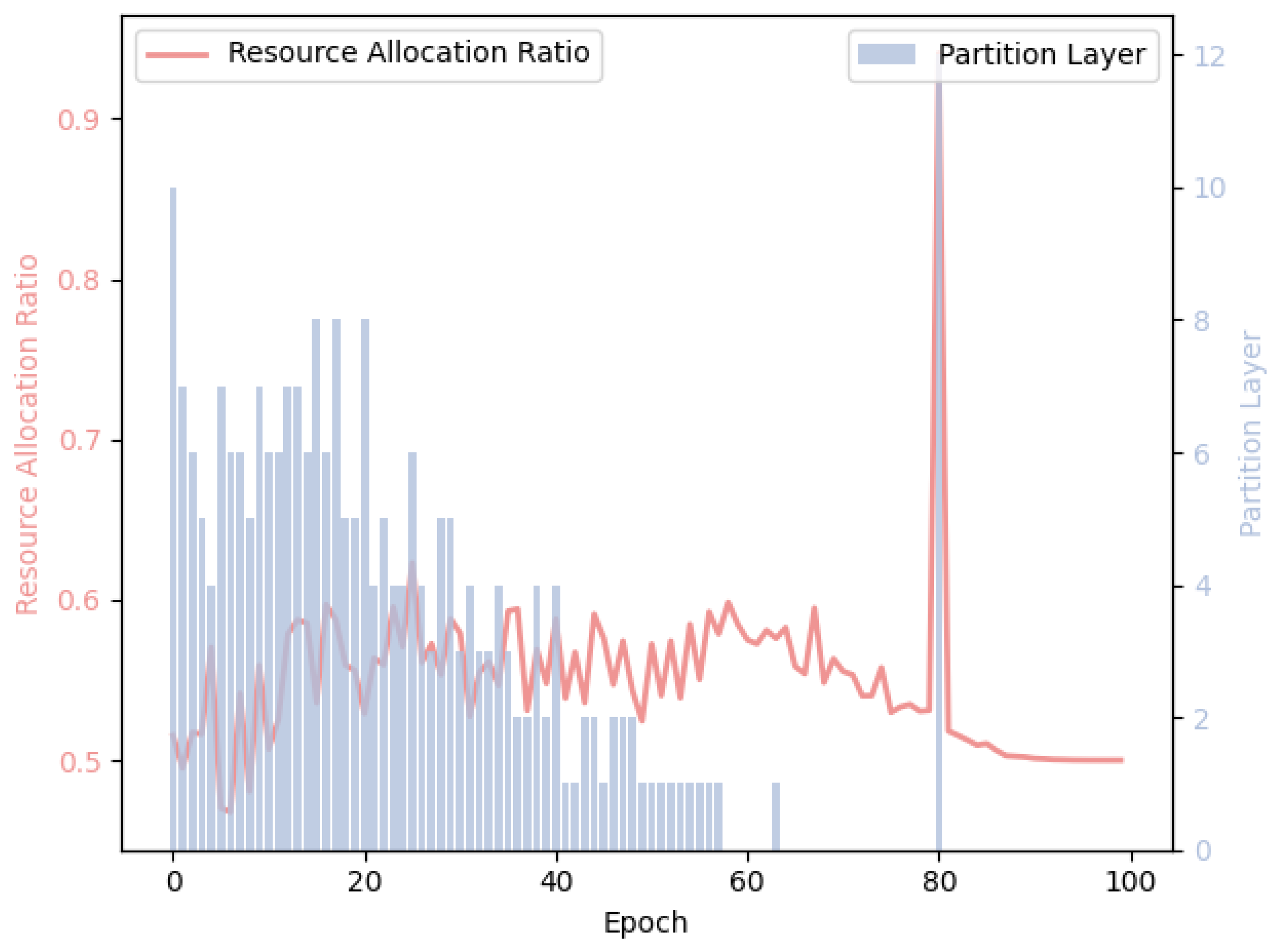
4.6. Training Process

As shown in Algorithm 1, during the training process, the parameters of the policy network and value network are first initialized. Then, in each iteration, the agent interacts with the environment to collect data, computes the reward for each state, and selects actions based on the output of the policy network. The policy is updated using the policy gradient method, while the value network is employed to evaluate the value of each state, optimizing both the policy and the value function.

Algorithm 1 DRL-Based Joint Optimization Algorithm

Input:

FLOPs of each logical layer, $C_{i,j}^{\mathrm{logic}}$; FLOPs of each exit branch, $C_{i,j}^{\mathrm{exit}}$; The computation probability of each logical layer, $P_{i,j}^{\mathrm{logic}}$; The computation probability of each exit branch, $P_{i,j}^{\mathrm{exit}}$; Number of end devices, N; Number of logical layers, $L_i$; Device computational capability, $R_i^{\mathrm{device}}$; Edge server computational capability, $R_{\mathrm{edge}}$; Bandwidth, B; Device power consumption, ${\mathrm{pow}}_i^{\mathrm{device}}$; Transmission power, ${\mathrm{pow}}_i^{\mathrm{trans}}$; Intermediate data size, $W_i^{\left(h_i\right)}$; Weights for latency $\mu$ and energy $\nu$.

Output:

Optimized model partitioning layers, $H=\{h_1,h_2,\dots ,h_N\}$; Optimized resource allocation, $Y=\{y_1,y_2,\dots ,y_N\}$.   1: Initialize actor network $YH(·)$ and critic network $V(·)$;   2: Initialize replay buffer $M\leftarrow \varnothing$;   3: Initialize hyperparameters $\alpha ,\gamma ,ϵ,\lambda$;   4: for episode $e=1$ to $\max \_\mathrm{episodes}$ do   5:        Initialize state $s_0=\mathrm{environment}.\mathrm{reset}\left(\right)$;   6:        Initialize memory buffer $M=\varnothing$;   7:        for each time step $t=1$ to $\max \_\mathrm{timesteps}$ do   8:               Select action $a_t=[y_t,h_t]$ using the actor network;   9:               Execute action $a_t$, obtain next state $s_{t+1}$, and reward $r_t$; 10:               Store $(s_t,a_t,r_t,s_{t+1})$ in memory buffer M; 11:               if episode is done then 12:                    Compute discounted returns $G_t$ for each step t in M; 13:                    for each experience $(s_t,a_t,r_t,s_{t+1})$ in M do 14:                          Compute advantage $A_t=G_t-V\left(s_t\right)$; 15:                          Compute policy loss: $L_{\mathrm{policy}}=-log\left(YH\left(a_t\right|s_t)\right)·A_t$; 16:                          Compute value loss: $L_{\mathrm{value}}={(G_t-V\left(s_t\right))}^2$; 17:                          Update actor network: 18:                          $YH(·)\leftarrow YH(·)-\alpha ·\nabla L_{\mathrm{policy}}$; 19:                          Update critic network: 20:                          $V(·)\leftarrow V(·)-\alpha ·\nabla L_{\mathrm{value}}$; 21:                    end for 22:                    Clear memory buffer $M\leftarrow \varnothing$; 23:               end if 24:        end for 25: end for 26: Return optimized segmentation layers H and resource allocation Y;

5. Experimental Evaluation

5.1. Experimental Setup

We construct and implement simulation experiments to validate the effectiveness of the proposed joint optimization method for model partitioning and resource allocation in reducing inference latency and energy consumption. The experiments first simulate the complexity distribution of input samples from different end devices and characterize the complexity of task samples based on the exit distribution in the multi-exit DNN.

Specifically, we assume that all logical layers have exits and calculate the task exit rate $P_i(\mathrm{exit}=j)$, where $j=1,2,\dots ,L_i$ for each logical layer. Based on this, we adopt the exit configuration algorithm proposed in [19] to determine the required multi-exit DNN structure for each end device.

Based on the exit configuration, we calculate the probability of computations occurring at each logical layer and exit branch, denoted as $P_{(i,j)}^{\mathrm{logic}}$ and $P_{(i,j)}^{\mathrm{exit}}$, respectively. Finally, the model partitioning and resource allocation schemes are determined, and the inference costs for different schemes are compared to assess the performances of various methods.

This study designs and implements two sets of simulation experiments. The first set focuses on image object recognition tasks, using VGG16 [20] as the backbone network. It assumes that the edge server’s computational capability is 500 GFLOPS, and the number of end heterogeneous devices, N, is set to 5.

Table 2. Image experiment parameter settings.

${\mathbf{pow}}_{\mathit{i}}^{\mathbf{device}}$ (W)	${\mathbf{pow}}_{\mathit{i}}^{\mathbf{trans}}$ (W)	${\mathit{R}}_{\mathit{i}}^{\mathbf{device}}$ (GFLOPS)	${\mathit{P}}_{\mathit{i}}(\mathbf{exit}=\mathit{j})$
0.5	0.1	50	{10%, 8%, 2%, 15%, 0%, 7%, 5%, 6%, 3%, 2%, 28%, 12%, 2%}
0.8	0.15	80	{12%, 6%, 3%, 10%, 1%, 8%, 4%, 7%, 2%, 1%, 25%, 15%, 6%}
1.2	0.2	100	{9%, 7%, 4%, 14%, 0%, 6%, 5%, 8%, 3%, 2%, 27%, 10%, 5%}
1.5	0.3	150	{11%, 5%, 2%, 13%, 1%, 9%, 4%, 6%, 3%, 1%, 26%, 14%, 5%}
2.0	0.4	200	{11%, 1%, 0%, 0%, 0%, 0%, 4%, 6%, 3%, 30%, 26%, 14%, 5%}

provides detailed information about the assumed power, transmission frequency, computational capability, and task optimal exit distribution $P_i(\mathrm{exit}=j)$ for the heterogeneous end devices.

The second set of experiments targets video object recognition tasks, allowing tasks to skip unsuitable exits based on the exit situation of the previous frame. VGG16 is used as the backbone network, with the edge server’s computational capability remaining at 500 GFLOPS, and the number of end heterogeneous devices, N, is increased to 7. It is assumed that, except for the first and last exits, the probability of a task skipping the remaining exit branches is 50% of the probability of computation occurring at the next exit $j+1$ for a given exit j.

Table 3. Video experiment parameter settings.

${\mathbf{pow}}_{\mathit{i}}^{\mathbf{device}}$ (W)	${\mathbf{pow}}_{\mathit{i}}^{\mathbf{trans}}$ (W)	${\mathit{R}}_{\mathit{i}}^{\mathbf{device}}$ (GFLOPS)	${\mathit{P}}_{\mathit{i}}(\mathbf{exit}=\mathit{j})$
0.3	0.08	30	{15%, 10%, 5%, 20%, 2%, 8%, 6%, 7%, 4%, 3%, 30%, 15%, 1%}
0.6	0.12	60	{12%, 8%, 4%, 15%, 1%, 9%, 7%, 6%, 5%, 3%, 25%, 14%, 2%}
1.2	0.2	100	{10%, 7%, 3%, 14%, 2%, 8%, 6%, 5%, 4%, 3%, 26%, 12%, 3%}
2.0	0.3	120	{9%, 6%, 2%, 13%, 1%, 10%, 5%, 7%, 4%, 2%, 27%, 13%, 3%}
3.0	0.4	200	{8%, 5%, 1%, 12%, 0%, 11%, 7%, 6%, 3%, 2%, 28%, 14%, 2%}
4.0	0.5	250	{7%, 4%, 1%, 10%, 0%, 12%, 6%, 5%, 3%, 1%, 29%, 15%, 2%}
5.0	0.6	300	{6%, 3%, 0%, 8%, 0%, 13%, 7%, 5%, 2%, 1%, 30%, 16%, 2%}

provides the corresponding power, transmission frequency, computational capabilities, and task optimal exit distributions $P_i(\mathrm{exit}=j)$ for the heterogeneous end devices.

The strategy network (Actor–Critic network) used in this experiment consists of two fully connected hidden layers, containing 128 and 64 neurons, respectively, and employs the ReLU activation function to enhance the model’s non-linear expressiveness. The strategy output (Actor) generates a continuous action vector, while the value function (Critic) outputs the state value estimation for the current state. The training process follows the procedure outlined in Algorithm 1, with a total of 500 training epochs, each containing 400 iterations. The initial learning rate is set to 0.001; the Adam optimizer is used, with a discount factor $\gamma$ set to 0.99 and a clipping threshold $ϵ$ of 0.2. In the policy selection process, a combination of the $\epsilon$-greedy strategy and Gaussian noise mechanism is applied to enhance exploration. Furthermore, the weight coefficients for latency and energy consumption are set to $\mu =4$ and $\nu =1$, respectively. In the state space $s_i\left(t\right)$, $k=5$, meaning that the energy consumption and latency information from the most recent 5 time steps is retained. The parameter $\alpha$ in the reward function $g\left(t\right)$ is set to 10 to amplify the reward signal. To evaluate the model’s adaptability under different bandwidth conditions, we adjust the bandwidth and conduct experiments at 3, 10, 20, 30, 40, 50, 60, and 70 Mbps.

5.2. Baseline Comparisons

We denote the resource average allocation strategy as “EAR” (Equal Allocation of Resources) and compare the proposed model partitioning and resource allocation scheme with the following baseline approaches:

1.

ACO-device only-EAR: The DNN exits are configured as in [19], with all tasks processed by the end devices and the resources of the edge server evenly distributed across all devices.

2.

ACO-edge only-EAR: The DNN exits are configured as in [19], with all inference tasks offloaded to the edge server for processing, and the resources of the edge server are evenly allocated among the devices.

3.

SPINN [9]-EAR: Exits are set at intervals of 15% FLOPs computation, and the model is partitioned accordingly. Since the resource allocation issue is not considered, it is assumed that the resource allocation follows an even distribution.

4.

ACO-EAR: The DNN exits are configured as in [19], with the model partitioned using the strategy proposed in [9], and the resources are evenly distributed.

5.

FP-AR (Fixed Partitioning-Resource Allocation): This method optimizes resource allocation based on a fixed model partitioning scheme (in this experiment, the partitioning layer for each model is randomly set to 6). A total of 1000 exhaustive search iterations are conducted, and the optimal resource allocation scheme is selected.

5.3. Performance Evaluation

5.3.1. Performance Evaluation of Image Experiments

Figure 3 and Figure 4 illustrate the dynamic changes in average inference cost and cumulative reward over training epochs under a bandwidth condition of 20 Mbps. The trends in the data from the figures clearly indicate that the model begins to converge after approximately 100 training epochs. Specifically, the magnitude of updates to the model parameters gradually decreases as the number of training epochs increases, and the fluctuations in performance metrics significantly narrow. These characteristics suggest that the model is approaching a relatively stable state. Meanwhile, the cumulative reward function shows a steadily decreasing trend without noticeable fluctuations or abrupt changes.

To provide a clearer understanding of the agent’s learning behavior during training, Figure 5 illustrates the evolution of action selections for Device 1 over 100 training epochs under a network bandwidth of 20 Mbps. The results indicate that, due to its limited computational capacity, Device 1 exhibits a strong reliance on edge server resources for model inference. As training progresses, the selected model split layer consistently converges to 0. This outcome implies that, within the proposed algorithmic framework, the system adaptively offloads a greater portion of the model to the edge server for low-capability devices, thereby improving overall resource utilization and system performance.

The experimental results presented in Figure 6, Figure 7 and Figure 8 illustrate the comparison of various methods in terms of total inference delay, total energy consumption, and total cost under different bandwidth conditions. The detailed analysis of the results is as follows:

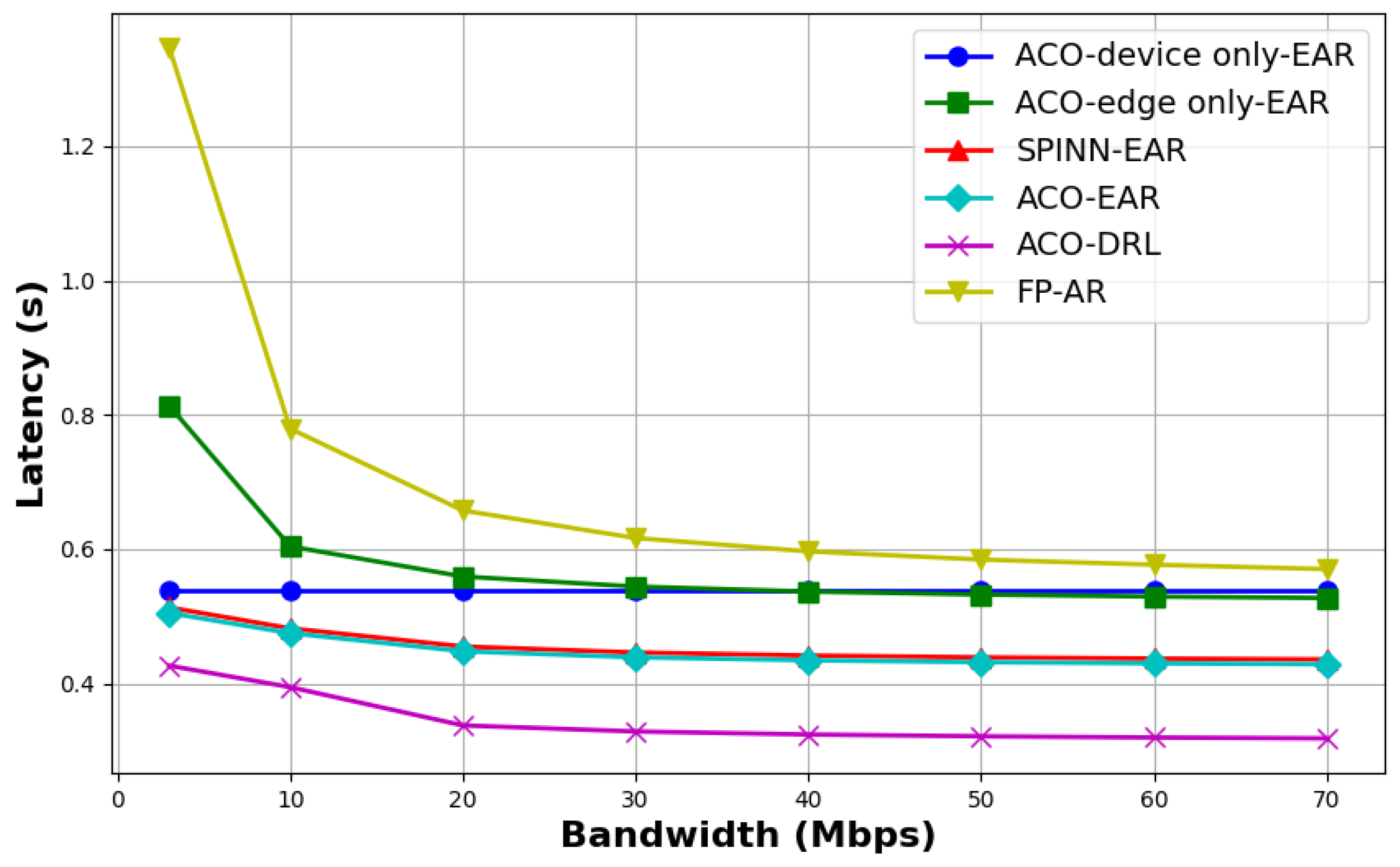
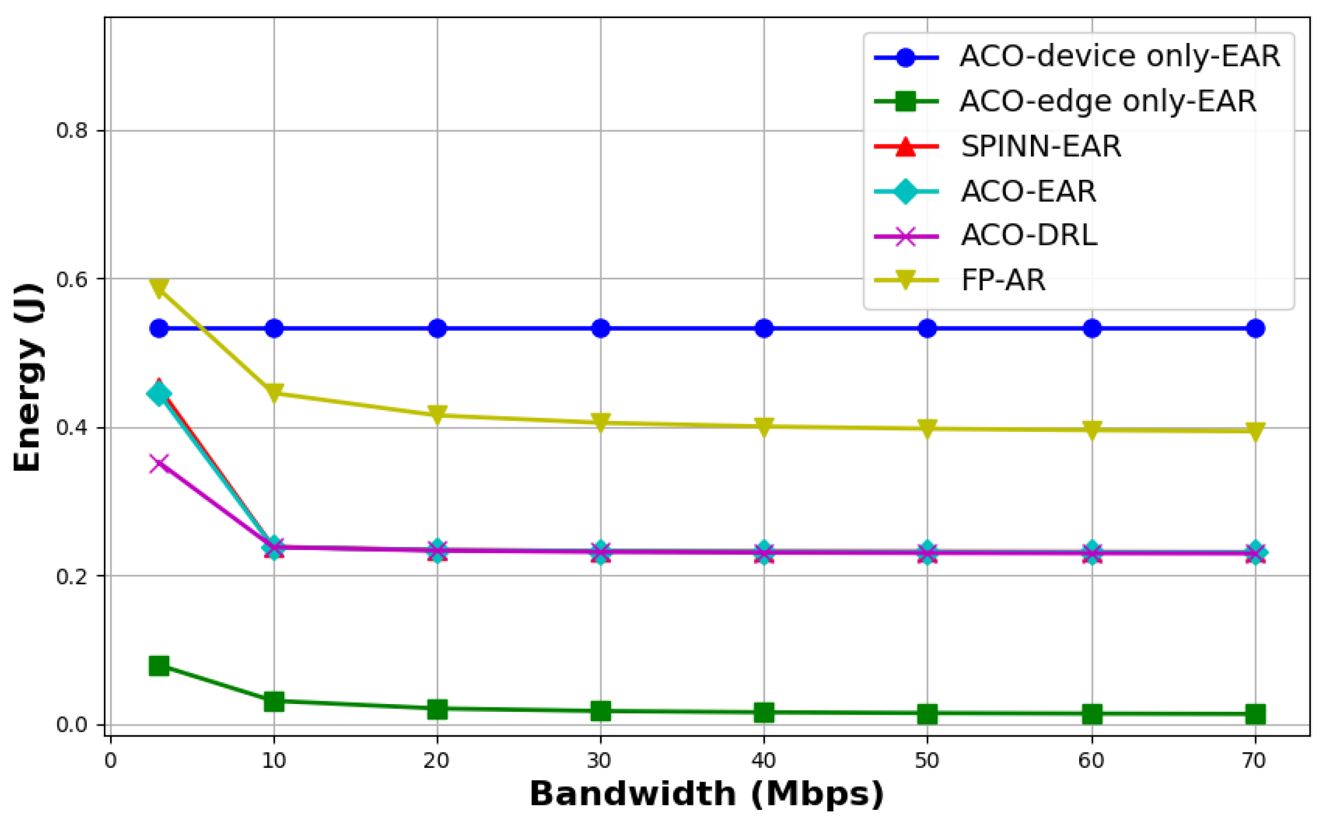
• “ACO-EAR” and “SPINN-EAR” adopt the same model partitioning strategy but are based on different exit-setting algorithms, with both employing an average resource allocation strategy. The experimental results indicate that “ACO-EAR” consistently achieves slightly lower inference delay, energy consumption, and cost compared with “SPINN-EAR”, demonstrating the impact of the exit-setting strategy on the inference performance of multi-exit DNNs.
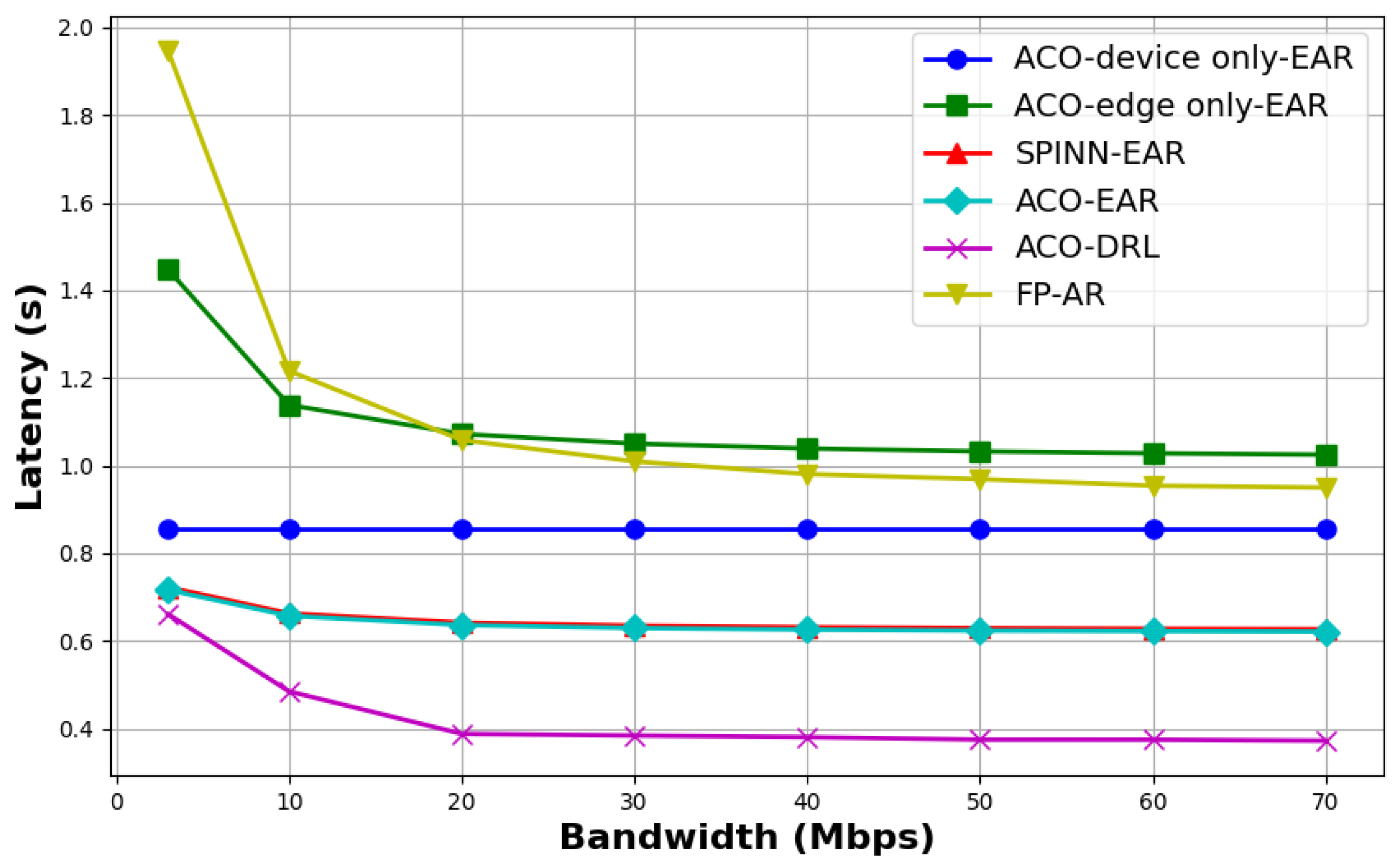
• Compared with the method adopting equal distribution of resources, “ACO-DRL” demonstrates superior performance in both inference latency and overall cost control, clearly highlighting the critical role of resource allocation strategies in enhancing inference efficiency.
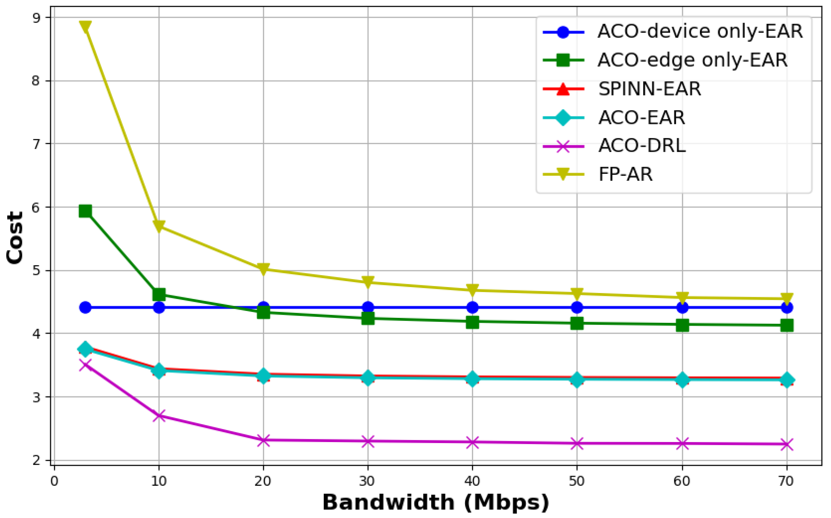
• “ACO-DRL” achieves joint optimization of both resource allocation and model partitioning strategies, whereas “FP-AR” only optimizes resource allocation based on a predefined fixed model partitioning scheme. Experimental results indicate that “ACO-DRL” consistently outperforms other methods in terms of latency and overall cost. In contrast, “FP-AR” shows inferior performance in both latency and cost control, and also exhibits higher energy consumption compared with most baseline methods. These findings validate the significant impact of model partitioning strategies on inference performance.
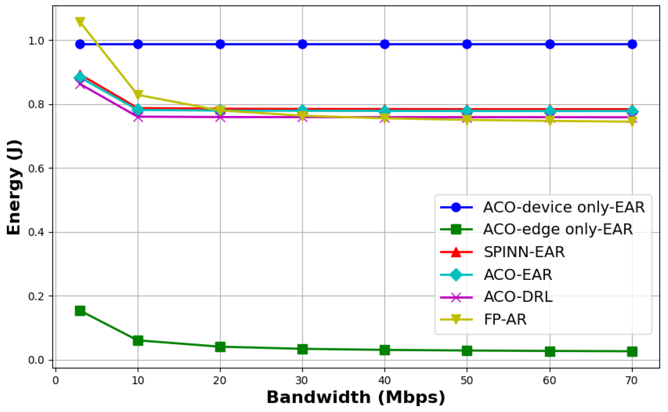
• Since “ACO-edge only-EAR” offloads all tasks to the edge server for inference, it consistently maintains the lowest energy consumption. However, under limited bandwidth conditions, this method results in considerable inference delay.
• When the bandwidth exceeds 10 Mbps, the energy consumption of “ACO-EAR” becomes comparable to that of “ACO-DRL”, suggesting that their model partitioning schemes are similar or identical. Nevertheless, since “ACO-DRL” further optimizes the resource allocation strategy, it achieves significantly better performance in terms of inference delay and overall cost than “ACO-EAR.”
• When the bandwidth exceeds 30 Mbps, the inference cost for all methods tends to stabilize. Among them, the proposed joint optimization method (“ACO-EAR”) consistently maintains the lowest inference cost, fully demonstrating the effectiveness of the proposed joint optimization algorithm for model partitioning and resource allocation.

5.3.2. Performance Evaluation of Video Experiments

Figure 9 and Figure 10 illustrate the evolution of the average inference cost and cumulative reward throughout the training process in the video-based experiment conducted under a bandwidth of 20 Mbps. Analysis indicates that the model converges after approximately 100 training episodes. Furthermore, the cumulative reward demonstrates a steadily declining trend without significant fluctuations, indicating stable learning behavior.

Under a bandwidth of 20 Mbps, Figure 11 shows the trajectory of action selection for Device 1 over the first 100 training epochs. The figure reveals that the action choices become progressively stable around the 80th epoch. Due to its limited local processing capacity, the device exhibits a clear tendency to rely on edge-side computation. This results in an increasing preference for allocating the entire inference task to the edge server, aiming to maintain stable and efficient performance during training.

The experimental results presented in Figure 12, Figure 13 and Figure 14 illustrate the performance of different methods in terms of total inference delay, total energy consumption, and total cost under varying bandwidth conditions. The detailed analysis is as follows:

• The performance of “ACO-EAR” and “SPINN-EAR” in terms of inference delay, energy consumption, and cost is comparable. However, owing to the more flexible exit-setting strategy adopted by “ACO-EAR,” it consistently achieves slightly better overall performance than “SPINN-EAR.”
• Compared with methods that do not incorporate resource optimization, “ACO-DRL” demonstrates superior performance in both inference latency and overall cost control, further confirming the significant impact of resource allocation strategies on the total system cost.
• Although the energy consumption of “FP-AR” is slightly lower than that of most methods when the bandwidth exceeds 40 Mbps, its latency is significantly higher than that of the majority of the other approaches, thereby demonstrating the critical importance of optimizing model partitioning decisions for inference performance.
• The “ACO-device only-EAR” and “ACO-edge only-EAR” methods underutilize the computational capabilities of either the edge server or the end device, respectively. As a result, their performance in terms of latency and overall cost is inferior to that of most other approaches.
• Under bandwidth-constrained conditions, the proposed method “ACO-DRL” achieves inference delay and cost comparable to or even better than other methods under sufficient bandwidth conditions. This further demonstrates the excellent adaptability of the proposed joint optimization method in varying network environments, effectively reducing inference costs and enhancing overall system performance.

6. Conclusions

In this paper, we investigate the joint optimization problem of model partitioning and resource allocation for multi-exit DNNs in an edge-device collaborative environment. We formulate a mathematical model with latency and energy consumption as the core optimization objectives and propose a joint optimization method based on DRL. Experimental results demonstrate that the proposed joint optimization algorithm significantly reduces inference costs, effectively validating its superiority in improving system performance.

References

1. LeCun, Y.; Bengio, Y.; Hinton, G. Deep Learning. Nature 2015, 521, 436–444. [Google Scholar] [CrossRef] [PubMed]
2. Teerapittayanon, S.; McDanel, B.; Kung, H.T. Branchynet: Fast Inference via Early Exiting from Deep Neural Networks. In Proceedings of the 23rd International Conference on Pattern Recognition (ICPR), Cancun, Mexico, 4–8 December 2016; pp. 2464–2469. [Google Scholar]
3. Mao, Y.; You, C.; Zhang, J.; Huang, K.; Letaief, K.B. A Survey on Mobile Edge Computing: The Communication Perspective. IEEE Commun. Surv. Tutor. 2017, 19, 2322–2358. [Google Scholar] [CrossRef]
4. Zhu, L.; Li, B.; Tan, L. A Digital Twin-based Multi-objective Optimized Task Offloading and Scheduling Scheme for Vehicular Edge Networks. Future Gener. Comput. Syst. 2025, 163, 107517. [Google Scholar] [CrossRef]
5. Ebrahimi, M.; Veith, A.D.; Gabel, M.; de Lara, E. Combining DNN Partitioning and Early Exit. In Proceedings of the 5th International Workshop on Edge Systems, Analytics and Networking, Rennes, France, 5–8 April 2022; pp. 25–30. [Google Scholar]
6. Li, N.; Iosifidis, A.; Zhang, Q. Graph Reinforcement Learning-based CNN Inference Offloading in Dynamic Edge Computing. In Proceedings of the IEEE Global Communications Conference (GLOBECOM), Rio de Janeiro, Brazil, 4–8 December 2022; pp. 982–987. [Google Scholar]
7. Xie, Z.; Xu, Y.; Xu, H.; Liao, Y.; Yao, Z. Collaborative Inference for Large Models with Task Offloading and Early Exiting. arXiv 2024, arXiv:2412.08284. [Google Scholar]
8. Bajpai, D.J.; Jaiswal, A.; Hanawal, M.K. I-splitee: Image Classification in Split Computing DNNs with Early Exits. In Proceedings of the IEEE International Conference on Communications (ICC), Denver, CO, USA, 9–13 June 2024; pp. 2658–2663. [Google Scholar]
9. Laskaridis, S.; Venieris, S.I.; Almeida, M.; Leontiadis, I.; Lane, N.D. SPINN: Synergistic Progressive Inference of Neural Networks Over Device and Cloud. In Proceedings of the 26th Annual International Conference on Mobile Computing and Networking (MobiCom), London, UK, 21–25 September 2020; ACM: New York, NY, USA, 2020; pp. 1–15. [Google Scholar]
10. Matsubara, Y.; Levorato, M.; Restuccia, F. Split Computing and Early Exiting for Deep Learning Applications: Survey and Research Challenges. ACM Comput. Surv. 2022, 55, 1–30. [Google Scholar] [CrossRef]
11. Zhou, M.; Zhou, B.; Wang, H.; Dong, F.; Zhao, W. Dynamic Path Based DNN Synergistic Inference Acceleration in Edge Computing Environment. In Proceedings of the 27th International Conference on Parallel and Distributed Systems (ICPADS), Beijing, China, 14–16 December 2021; pp. 567–574. [Google Scholar]
12. Kang, Y.; Hauswald, J.; Gao, C.; Rovinski, A.; Mudge, T.; Mars, J.; Tang, L. Neurosurgeon: Collaborative Intelligence Between the Cloud and Mobile Edge. In Proceedings of the 22nd International Conference on Architectural Support for Programming Languages and Operating Systems (ASPLOS), Xi’an, China, 8–12 April 2017; pp. 615–629. [Google Scholar]
13. Liu, Z.; Lan, Q.; Huang, K. Resource Allocation for Batched Multiuser Edge Inference with Early Exiting. In Proceedings of the IEEE International Conference on Communications (ICC), Rome, Italy, 28 May–1 June 2023; pp. 3614–3620. [Google Scholar]
14. Cao, Y.; Fu, S.; He, X.; Hu, H.; Shan, H.; Yu, L. Video Surveillance on Mobile Edge Networks: Exploiting Multi-Exit Network. In Proceedings of the IEEE International Conference on Communications (ICC), Rome, Italy, 28 May–1 June 2023; pp. 6621–6626. [Google Scholar]
15. Dong, F.; Wang, H.; Shen, D.; Huang, Z.; He, Q.; Zhang, J.; Wen, L.; Zhang, T. Multi-exit DNN Inference Acceleration Based on Multi-dimensional Optimization for Edge Intelligence. IEEE Trans. Mob. Comput. 2022, 22, 5389–5405. [Google Scholar] [CrossRef]
16. Kim, J.W.; Lee, H.S. Early Exiting-aware Joint Resource Allocation and DNN Splitting for Multi-sensor Digital Twin in Edge-cloud Collaborative System. IEEE Internet Things J. 2024, 11, 36933–36949. [Google Scholar] [CrossRef]
17. Liu, Z.; Song, J.; Qiu, C.; Wang, X.; Chen, X.; He, Q.; Sheng, H. Hastening Stream Offloading of Inference via Multi-exit DNNs in Mobile Edge Computing. IEEE Trans. Mob. Comput. 2022, 23, 535–548. [Google Scholar] [CrossRef]
18. Li, E.; Zeng, L.; Zhou, Z.; Chen, X. Edge AI: On-demand Accelerating Deep Neural Network Inference via Edge Computing. IEEE Trans. Wirel. Commun. 2019, 19, 447–457. [Google Scholar] [CrossRef]
19. Ma, Y.; Tang, B. Correlation-Aware Exit Setting for Deep Neural Network Inference. In Proceedings of the 2024 4th International Conference on Digital Society and Intelligent Systems (DSIns), Sydney, Australia, 20–22 November 2024. [Google Scholar]
20. Simonyan, K.; Zisserman, A. Very Deep Convolutional Networks for Large-Scale Image Recognition. arXiv 2014, arXiv:1409.1556. [Google Scholar]
Figure 1. An illustration of the end-edge collaborative scenario.
Electronics 14 01647 g001
Figure 2. Composition diagram of cost function.
Electronics 14 01647 g002
Figure 3. The dynamic evolution of the average cost in the image experiment (bandwidth of 20 Mbps).
Electronics 14 01647 g003
Figure 4. The dynamic evolution of the cumulative reward in the image experiment (bandwidth of 20 Mbps).
Electronics 14 01647 g004
Figure 5. Action decisions of Device 1 in 100 epochs during image experiments (bandwidth of 20 Mbps).
Electronics 14 01647 g005
Figure 6. Processing latency of different methods in image experiments.
Electronics 14 01647 g006
Figure 7. Energy consumption performance of different methods in image experiments.
Electronics 14 01647 g007
Figure 8. Cost of different methods in image experiments.
Electronics 14 01647 g008
Figure 9. The dynamic evolution of the average cost in the video experiments (bandwidth of 20 Mbps).
Electronics 14 01647 g009
Figure 10. The dynamic evolution of the cumulative reward in the video experiments (bandwidth of 20 Mbps).
Electronics 14 01647 g010
Figure 11. Action decisions of Device 1 in 100 epochs during video experiments (bandwidth of 20 Mbps).
Electronics 14 01647 g011
Figure 12. Processing latency of different methods in video experiments.
Electronics 14 01647 g012
Figure 13. Energy consumption performance of different methods in video experiments.
Electronics 14 01647 g013
Figure 14. Cost of different methods in video experiments.
Electronics 14 01647 g014