Eco-Cooperative Planning and Control of Connected Autonomous Vehicles Considering Energy Consumption Characteristics

Abstract

Cooperative driving systems can coordinate individual vehicles on the road in a platoon, holding significant promise for enhancing traffic efficiency and lowering the energy consumption of vehicle movements. For an extended period, vehicles on the road will consist of a mix of traditional gasoline and electric vehicles. To explore the economic driving strategies for diverse vehicles on the road, this paper introduces a collaborative eco-driving system that takes into account the energy consumption traits of vehicles. Unlike prior research, this paper puts forward a lane change decision-making approach that integrates energy modeling and speed prediction. This method can effectively capture the speed variations in the vehicle ahead and facilitate lane changes with energy efficiency in mind. The system encompasses three vital functions: vehicle cooperative architecture, ecological trajectory planning, and power system control. Specifically, eco-speed planning is carried out in two stages: the initial stage is executed globally, with cooperative speed optimization performed based on the energy consumption characteristics of different vehicles to determine the economical speed for vehicle platoon driving. The subsequent stage involves local speed adaptation, where the vehicle platoon dynamically adjusts its speed and makes lane change decisions according to local driving conditions. Ultimately, the generated control information is fed into the powertrain control system to regulate the vehicle. To assess the proposed collaborative eco-driving system, the algorithms were tested on highways, and the results substantiated the system’s efficacy in reducing the energy consumption of vehicle driving.

1. Introduction

As the number of registered vehicles rises and transportation demand grows, traditional traffic management and energy sustainability face substantial challenges [1,2]. To enhance energy efficiency and foster sustainable transportation, the automotive industry has been vigorously developing electric vehicles to cut down on petroleum consumption. The coexistence of electric and fuel-powered vehicles on the road has become a prevalent situation. Another way to lower fuel consumption is by optimizing vehicle dynamics to boost energy efficiency. With the help of advanced vehicle-to-everything (V2X) technologies, connected and automated vehicles (CAVs) can gather information on surrounding roads and traffic conditions. Consequently, they can operate in a coordinated fashion to improve driving safety, economic efficiency, and road capacity [3,4].

When self-driving technology is applied to vehicle formations, multiple self-driving vehicles can work together in a platoon to maintain tighter vehicle spacing, which reduces air resistance, improves driving efficiency, reduces traffic congestion, and thus improves overall energy efficiency [5,6]. For decades, researchers have made numerous attempts at vehicle formation, and experimental results have demonstrated that vehicle formation improves fuel economy by 6–10% due to reduced air resistance and unnecessary acceleration and deceleration operations [7]. As a result, interest in platoon energy consumption has increased considerably in recent years, with the research literature focusing on two main areas. One approach is to investigate platoon cruising speed planning in specific scenarios, aiming to lower vehicle energy use through speed control [8,9,10,11]. The other is to achieve energy savings at the control level by creating vehicle eco-driving controllers using vehicle energy consumption models. This enhances the platoon’s overall efficiency while maintaining tracking effectiveness [12,13,14,15]. The third is to study suitable energy management strategies to save energy from the characteristics of the vehicle powertrain [16,17].

Energy optimization is a critical aspect of decision-making and planning for self-driving vehicles. Speed planning scenarios primarily focus on key factors such as road geometry (including slope, curvature, and condition), traffic signal status, and the position of the leading vehicle. These elements significantly influence the energy efficiency of vehicle platoons in real-world driving conditions [18,19]. Many studies have been conducted to capture the gradient changes during driving through high-precision maps and gradient prediction to increase the power output when traveling uphill and reduce the power demand using gravity to improve driving economy when traveling downhill [8,20,21,22,23]. Another perspective is to adjust the vehicle headway during ramp driving to reduce the acceleration and braking demand of the vehicle on the ramp to maintain the optimal driving condition on the ramp and reduce the fuel consumption and emission [9,24]. In the case of signalized intersections, real-time planning of platoon economic speeds through algorithms such as dynamic planning allows the vehicle platoon to pass through the intersection more smoothly during the signal cycle, thus improving capacity and reducing energy consumption [10,11,25,26]. Due to the prevalence of mixed traffic on roads, optimal speeds for mixed vehicles need to be considered in an integrated manner in order to minimize the overall energy consumption based on the energy consumption characteristics of different vehicles [27,28,29]. However, eco-driving schemes for speed planning are generally more ideal, planning only the longitudinal speed of vehicles, thus making it difficult to characterize stochastic microscopic traffic conditions.

In this paper, we take a highway scenario as the object of study and consider the lane-changing behavior of a vehicle platoon that encounters interference from the vehicle in front of it, as well as the stochastic formation behavior of the vehicle platoon on the road. The merging and splitting of vehicle platoons require a unified cooperative driving framework for their description. Wang et al. developed a cooperative maneuver model for single-vehicle cruising and multi-vehicle platoon switching based on a hybrid automata architecture. They verified the framework’s effectiveness in several typical scenarios [30]. Ma et al. proposed a hybrid multimodal vehicle cooperative driving control architecture, demonstrating the simulation of vehicle platoon cruising, following, lane changing, overtaking, and entering/exiting garage functions under different traffic conditions [31]. While traveling, vehicles always seek more efficient passing or energy-saving driving by changing lanes or overtaking. Therefore, only the longitudinal speed planning of the considered vehicles is not enough. A complete lane change process consists of three parts: lane change decision, trajectory planning, and control execution. A lane change decision is a process whereby the system evaluates whether a lane change should be made based on the traffic around the vehicle, considering the impact of many factors, such as safety, driver personality, lane efficiency, and energy cost [32,33]. Effective lane-changing decisions can significantly improve the vehicle’s fuel economy [34]. Trajectory planning mainly ensures the continuity and comfort of the lane change curve [35]. In summary, existing studies mostly consider the ecological driving strategies of vehicles in specific road scenarios, and they lack trajectory planning for vehicles from the perspective of energy consumption of a mixed platoon, considering the stochastic traffic conditions on the road. In order to fill this gap, it is necessary to develop a vehicle cooperative eco-driving system that enables CAVs to flexibly handle split and merge operations between platoons, and queue speed planning by considering the energy consumption characteristics of all vehicles in a mixed platoon, as well as lane-changing operations based on stochastic traffic conditions on the road.

The primary aim of this research is to develop a vehicle cooperative eco-driving system for coordinated driving and eco-trajectory planning of CAVs in road traffic scenarios. The key contributions of this study are as follows: (1) A vehicle cooperative driving system based on hybrid automata is designed, enabling flexible switching and transition of vehicle maneuvers such as merging and dissolving. (2) An energy consumption model is established according to the energy characteristics of different vehicles, and the optimal cruising speed is determined by considering all vehicles in the CAV platoon. (3) Economical lane change decisions are provided when encountering the vehicle ahead, thus further reducing driving energy consumption. The lane change trajectory is optimized to ensure comfort and efficiency during the lane change process.

The rest of this paper is structured as follows. Section 2 outlines the overall framework of the vehicle eco-coordination system. Section 3 details the method for calculating the economic speed for vehicle platoons. Section 4 presents the driving planning approach for the vehicle platoon. Section 5 discusses the design of the vehicle platoon tracking controller. Section 6 explains the hybrid automata-based modeling technique for vehicle cooperative systems. Section 7 provides the simulation experiments and results. The conclusion is in the final section.

2. System Architecture

2.1. System Operating Environment

With the convergence of intelligent and interconnected technologies like DSRC, V2X, and others, CAVs can communicate with each other and exchange data with the road infrastructure, enabling more intelligent traffic management and vehicle control [36,37]. This information transmission and vehicle control in real time or near real time allows vehicles to more accurately perceive their surroundings, make appropriate decisions, and interact effectively with other vehicles and traffic signal systems. Consequently, the collaborative eco-driving system discussed in this paper is based on the following assumptions:

(1)

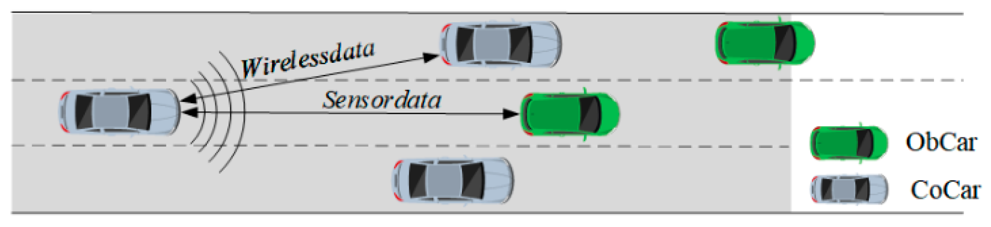
Road system: CAVs driving on roads provided with communication infrastructure. The road system communications infrastructure enables functions related to information sense, transmission, computation, storage, and control.

(2)

Information communication: CAVs can sense, transmit, and receive information about the driving environment and vehicle control in real-time with negligible delay in information communication.

(3)

Vehicle control: CAVs can accurately control the state of the CAV’s movement and are equipped with a formation system that allows them to drive in adaptive cruise control and formation with other CAVs. Vehicle platoon control is based on a distributed control framework, where each vehicle can autonomously regulate its driving behavior according to dynamic conditions.

2.2. Overall Framework

In this paper, a vehicle cooperative eco-driving system is designed based on a hybrid automata architecture, as shown in Figure 1, which consists of three main functions: (1) cooperative operation of the cooperative driving system, (2) vehicle cooperative speed planning, and (3) path tracking and vehicle control.

(1)

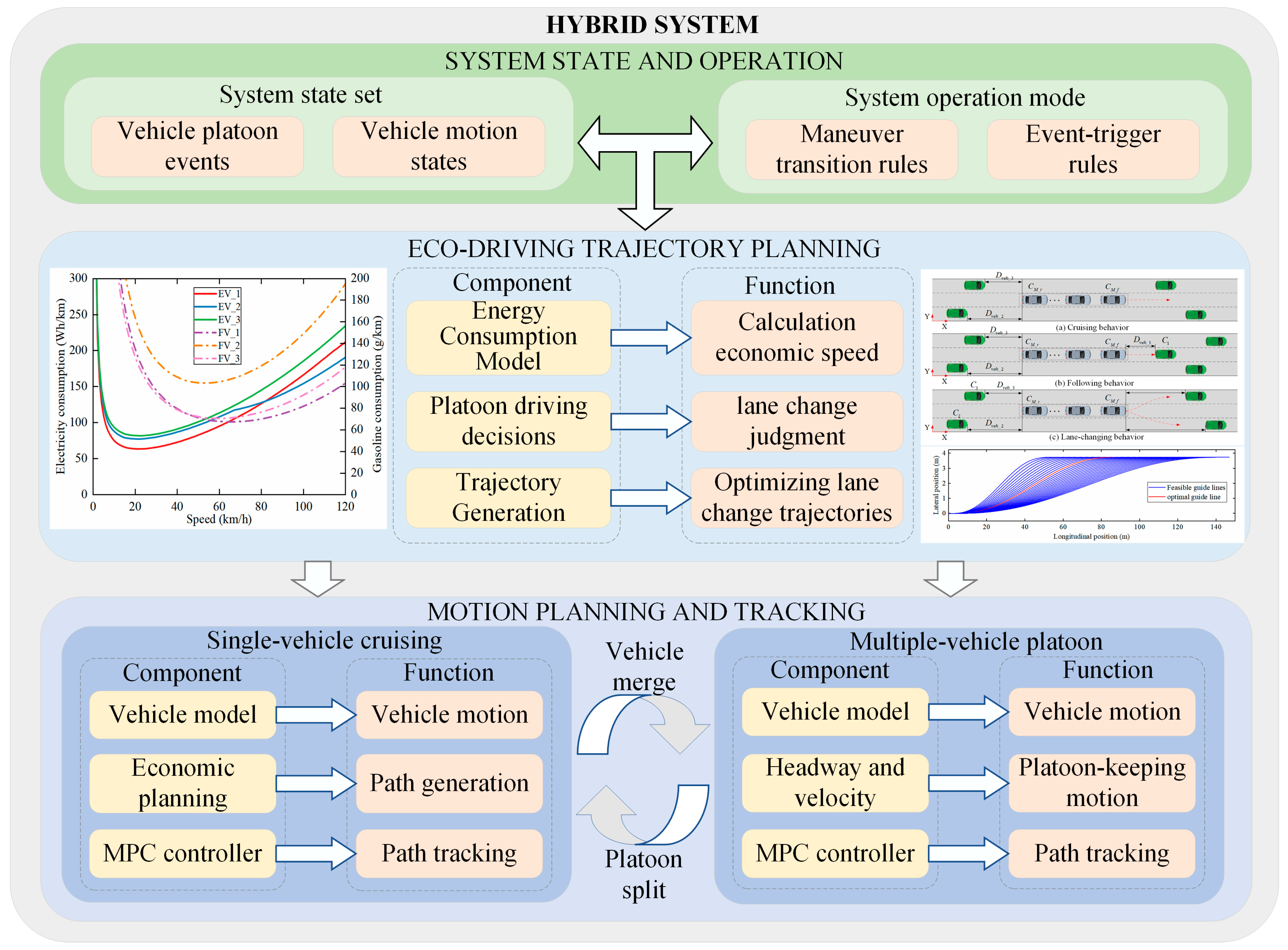
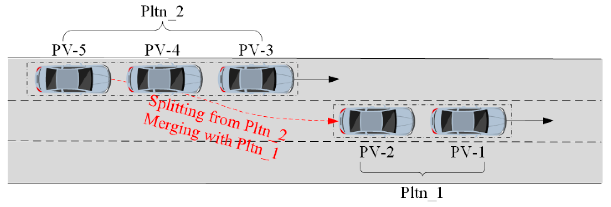
As the core of coordinating various functional modules, the cooperative driving system’s collaborative operation includes a control architecture that encompasses two key components: the state set and the operation mode. The state set characterizes the motion status and attributes of both the controlled vehicles and the surrounding environment. The operation mode outlines the transition rules for maneuvers between individual vehicle cruising and platooning, specifies the triggering mechanisms for platoon splitting and merging, and manages the formation and dissolution of vehicle groups.

(2)

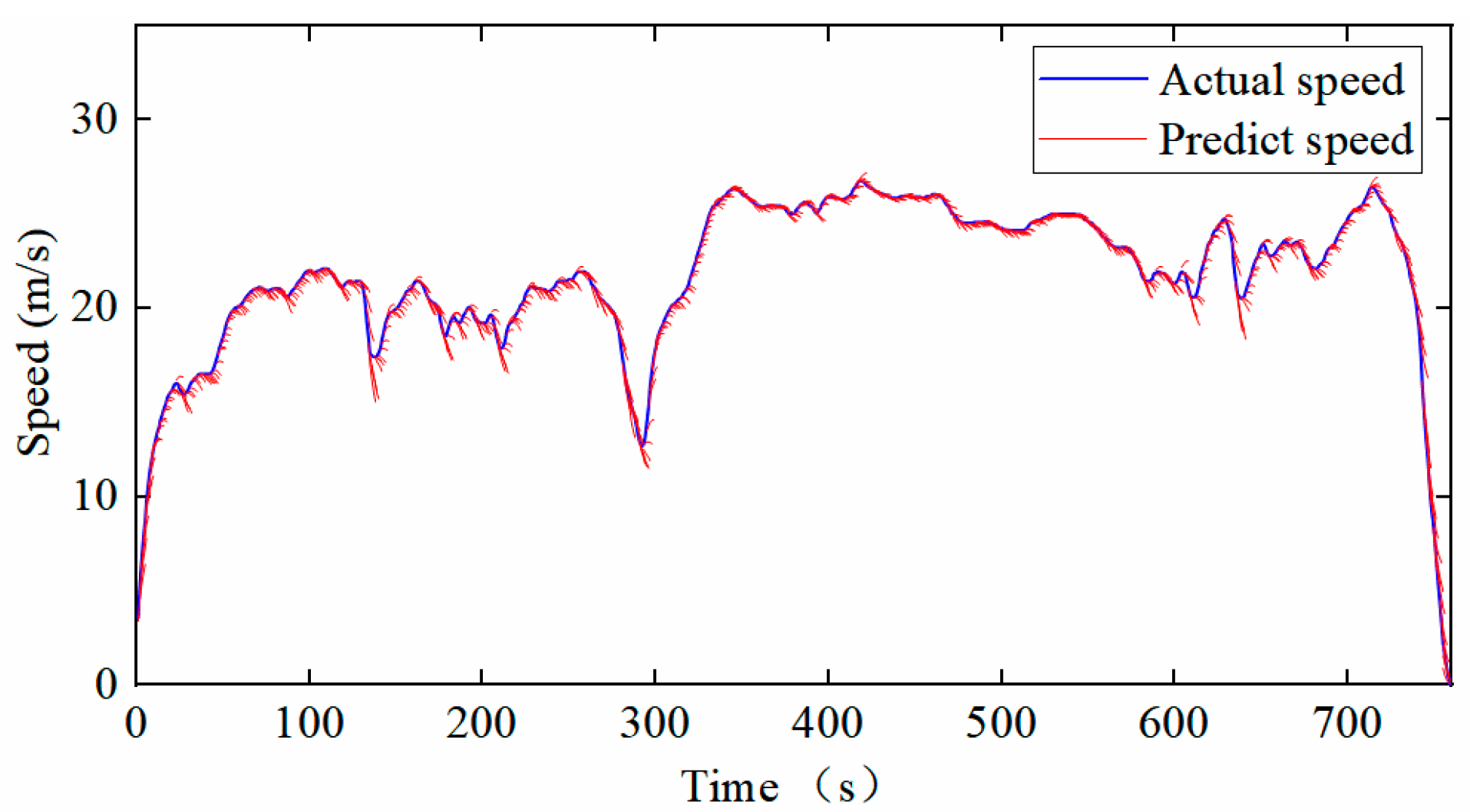
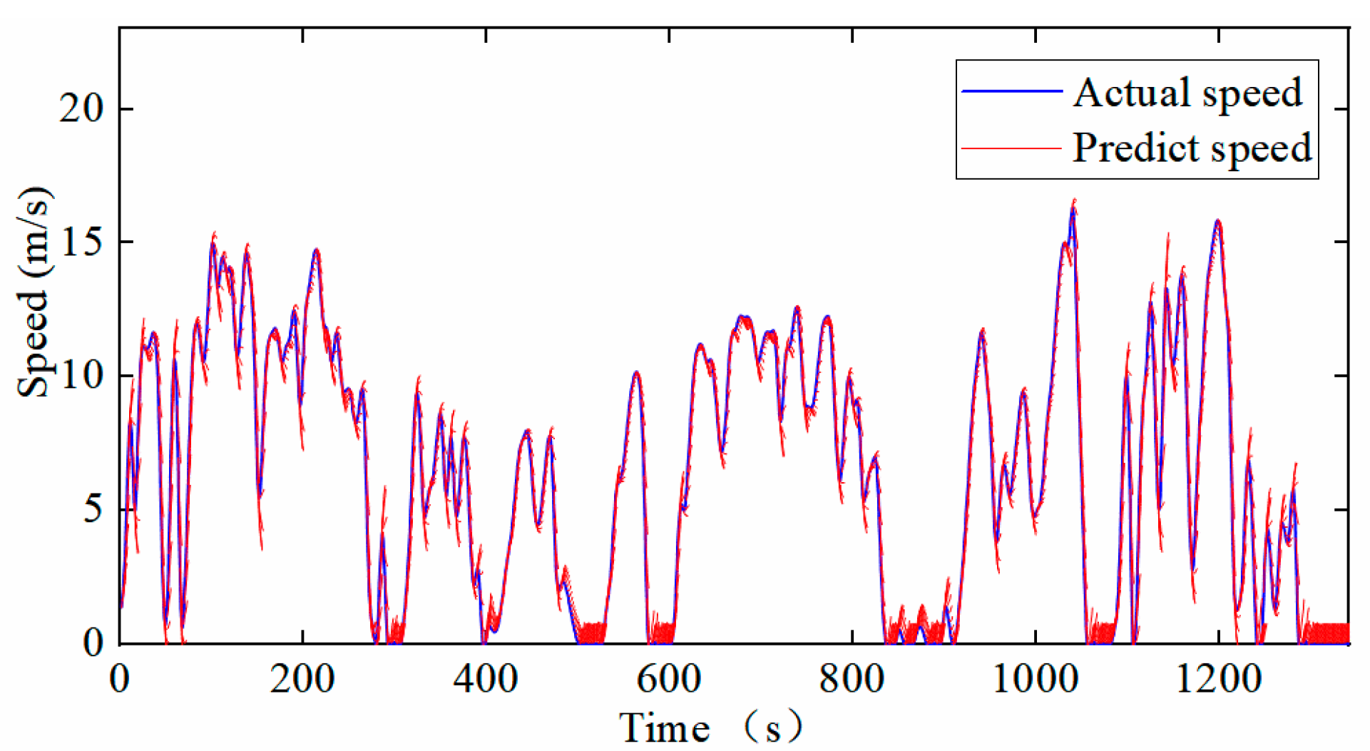
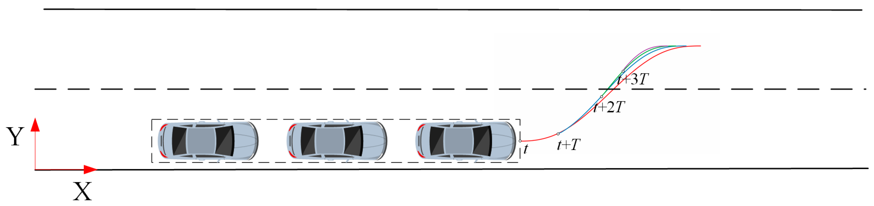
Vehicle cooperative speed planning is the core content of the cooperative eco-driving system, mainly containing two key aspects. First, the driving system plans the economic speed for cooperative driving according to the energy consumption characteristics of all vehicles in the vehicle platoon. It optimally adjusts it globally to minimize the overall energy consumption. Second, when encountering the vehicle ahead, the system will forecast the future speed of the vehicle via the RBF neural network while ensuring safety. It will then make intelligent energy-saving lane-changing decisions and optimize the lane-changing path to ensure both the efficiency of lane-changing and passenger comfort.

(3)

The aim of trajectory tracking is to ensure vehicles adhere to a pre-planned path accurately and swiftly. Within a vehicle platoon, the lead vehicle’s control goal is to track the planned reference trajectory, whereas the follower vehicle’s control goal is to track the lead vehicle’s path and maintain proper platoon spacing. In this paper, distinct controllers for the lead and follower vehicles are constructed using the MPC method to achieve vehicle following and formation maintenance based on their respective control objectives.

3. Calculation of Economic Cruising Speed Considering Energy Consumption Characteristics

Considering that a mix of traditional fuel vehicles and electric vehicles will coexist on the road for extended periods in the future, self-driving vehicles need to adapt to different vehicle types and intelligent interaction systems to ensure safe and efficient cooperative driving with various vehicles. Therefore, to perform economic driving planning for vehicle platoons, different energy consumption models are developed to forecast vehicle energy use based on the distinct energy consumption traits of traditional fuel and electric vehicles.

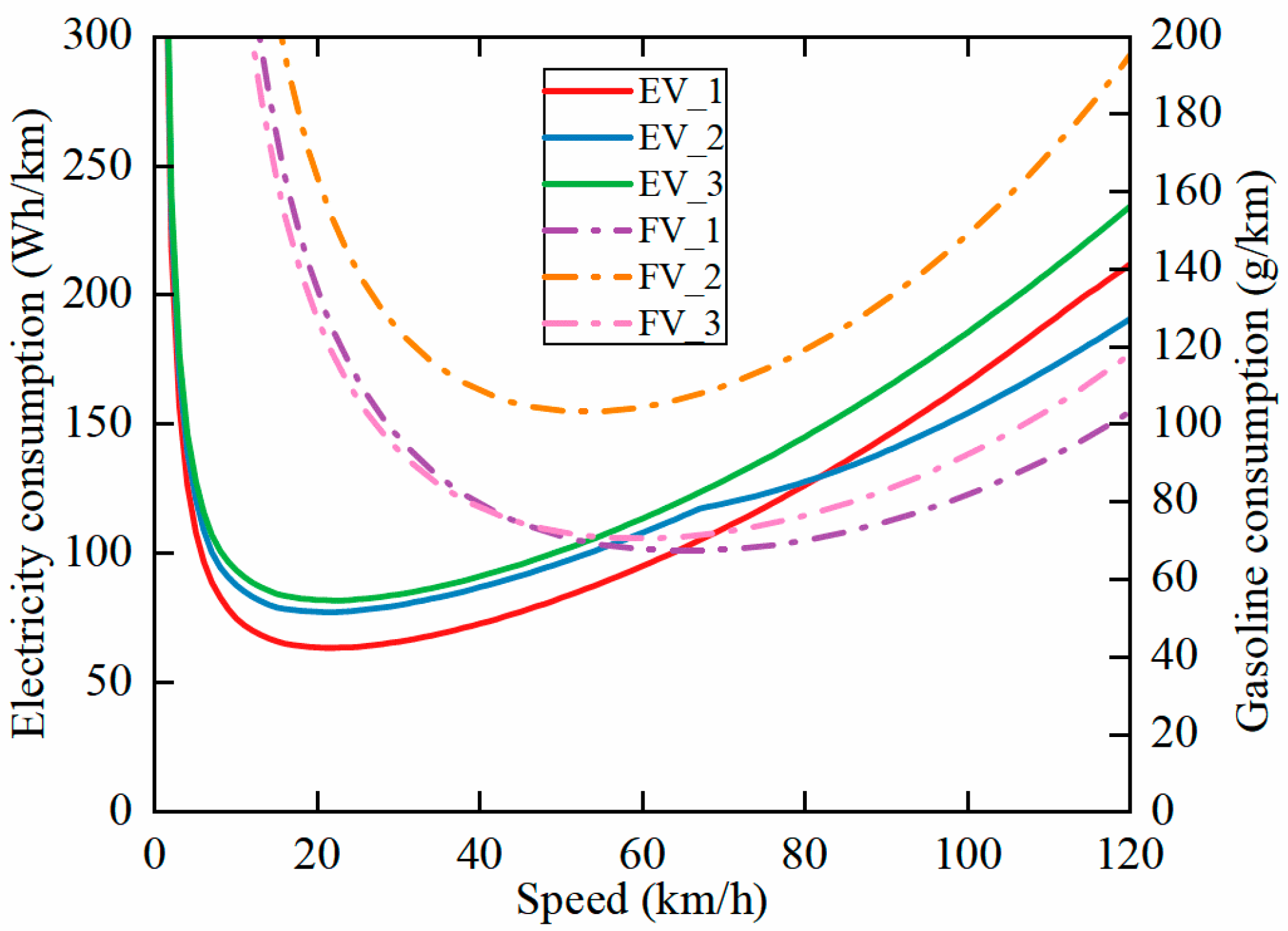
3.1. Fuel Vehicle Energy Consumption Model

The power $P_{wheel}(t)$ applied to the vehicle driveline at the wheel at the moment, $t$, is calculated by the longitudinal dynamics model:

$$P_{wheel}(t)=(mg\sin (\theta )+mgf\cos (\theta )+{\displaystyle \frac{1}{2}}\rho C_{d}A{v}^2(t)+ma(t))\cdot v(t)$$

(1)

where $m$ is the mass of the vehicle; $g$ is the acceleration due to gravity; $\theta$ is the road slope; $\rho$ is the air density; $C_d$ is the air resistance coefficient; $A$ is the windward area; $v(t)$ and $a(t)$ are the speed and acceleration of the vehicle at moment $t$, respectively; and $f$ is the rolling resistance coefficient.

The VT-CPFM-1 model was used to estimate real-time fuel consumption rates for fuel-guzzling vehicles and can be calibrated using data from city and highway fuel economy ratings published by the U.S. Environmental Protection Agency (EPA) [38]. Moreover, the required parameters are simple and can be obtained from major automotive websites, so the model was used to estimate the energy consumption of fuel vehicles:

$$FC(t)=\left\{\begin{array}{ll}{\alpha }_0+{\alpha }_1{P}_{wheel}(t)+{\alpha }_2{P}_{wheel}{(t)}^2& P_{wheel}(t)\ge 0\\ {\alpha }_0& P_{wheel}(t)<0\end{array}\right.$$

(2)

where $FC(t)$ is the fuel consumption rate (L/s) of the fuel vehicle at moment, $t$; ${\alpha }_i,i=0,1,2,3$ is a vehicle-specific model constant based on per-vehicle calibration; ${\alpha }_0$ represents the fuel consumption rate of the vehicle in the idling state, which is calibrated using the vehicle engine parameters as well as the fuel consumption in the EPA urban and highway driving cycles; ${\alpha }_2$ represents the constant related to the square of the power to ensure the calculation of energy consumption of the model under extreme conditions; and ${\alpha }_1$ ensures the linear relationship between the power and the fuel consumption.

3.2. Electric Vehicle Energy Consumption Model

The CPEM model, which was validated using data collected using the Advanced Vehicle Testing Activity (AVTA) at the U.S. Department of Energy’s Idaho National Laboratory (INL), was used to estimate the real-time energy consumption of electric vehicles [39]. The driving resistance of an electric vehicle on the road is basically the same as that of a fuel vehicle, so the power, $P_{wheel}$, at the wheels of an electric vehicle can be calculated by Equation (1), and the energy consumption, $P_{total}$, of an electric vehicle during driving can be calculated by the following equation:

$$P_{total}(t)=\left\{\begin{array}{ll}{P}_A(t)+{\displaystyle \frac{P_{wheel}(t)}{\eta }}& P_{wheel}(t)\ge 0\\ P_A(t)+P_{wheel}(t)\cdot \eta \cdot {\eta }_{rb}(t)& P_{wheel}(t)<0\end{array}\right.$$

(3)

where $P_A$ is the power consumed by the vehicle auxiliary system, such as on-board electrical equipment, air conditioning, etc., and the auxiliary system load is generally assumed to be 700 W; and $\eta$ is the series of losses experienced by the battery power when it is transmitted to the wheels through the vehicle powertrain, which is defined as the product of the vehicle transmission efficiency, the electric motor efficiency, and the battery efficiency. Moreover, ${\eta }_{rb}(t)$ is the regenerative braking recovery efficiency of the electric vehicle, which presents a characteristic similar to the exponential function with the negative acceleration of the vehicle during braking. It can be calculated from the current braking acceleration of the vehicle:

$${\eta }_{rb}(t)={\left[e^{\left({\displaystyle \frac{\alpha }{|a(t)|}}\right)}\right]}^{-1}$$

(4)

where $a(t)$ is the vehicle acceleration, and $\alpha$ is the fitting coefficient for the regenerative braking efficiency.

3.3. Calculation of Optimum Cruising Speed

The energy consumption per unit distance serves as an indicator of the vehicle’s economic cruising speed. Based on the energy consumption models established for both fuel and electric vehicles, the energy consumption per unit distance at various cruising speeds can be determined using the following equation:

$$Q=\left\{\begin{array}{l}{\displaystyle \frac{3600}{v}}({\alpha }_0+{\alpha }_1{P}_{wheel}(t)+{\alpha }_2{P}_{wheel}{(t)}^2)G_k\\ {\displaystyle \frac{3600}{v}}\left(P_A(t)+{\displaystyle \frac{P(t)}{\eta }}\right)\end{array}\right.$$

(5)

where $Q$ is the energy consumption per unit distance (kwh/km); and $G_k$ is the energy conversion ratio of gasoline to electrical energy, as specified by the EU standard, which is about 8.6 kWh for 1 L of gasoline.

In this section, three fuel and three electric vehicles are considered, and their types and parameters are shown in

Table 1. Vehicle parameters.

Type	Mass (kg)	Drag Coefficient	Frontal Area (m2)
EV_1	1417	0.29	2.38
EV_2	1794	0.26	2.36
EV_3	2124	0.28	2.54
FV_1	1500	0.28	2.424
FV_2	2190	0.31	2.911
FV_3	1453	0.30	2.32

. The energy consumption per unit distance for different types of vehicles is shown in Figure 2.

The closer proximity of the rear vehicle to the front vehicle within the vehicle platoon, which is located within the air drag zone behind the vehicle in front of it, results in a reduction in the drag area of the rear vehicle and a change in the airflow, which in turn results in the air drag coefficient that will change. In order to accurately capture this change, a correction formula is introduced [40]:

$$C_i(d)=\left\{\begin{array}{cc}{C}_d& i=1\\ C_d(1-{\displaystyle \frac{{\beta }_1}{{\beta }_2+d_i}})& i>1\end{array}\right.$$

(6)

where $C_i(d)$ represents the air resistance coefficient of the vehicle in the vehicle platoon, $C_d$ is the nominal air resistance coefficient, $i=1$ represents the leading vehicle, $i>1$ represents the following vehicle, ${\beta }_1$ and ${\beta }_2$ are the fitting constants, and $d_i$ represents the inter-vehicle distance from the preceding vehicle.

While a vehicle platoon travels on the road, the energy consumption per unit distance of each vehicle fluctuates due to variations in air resistance. The platoon shares vehicle parameter information via inter-vehicle communication and acquires road speed-limit data from the cloud. Utilizing the previously established vehicle energy consumption model, we can determine the overall energy consumption per unit distance for the platoon on the road.

$$Q_{platoon}={\displaystyle {\sum }_{i=1}^{n}Q(C_i(d))}$$

(7)

The vehicle speed limit is used as a constraint and traversed to obtain the economic driving speed of the vehicle platoon:

$$v_{eco}=find\min (Q_{platoon}(v)(v_{\lim \_\min }\le v\le v_{\lim \_\max }))$$

(8)

where $v_{\lim \_\min }$ and $v_{\lim \_\max }$ are the minimum and maximum values of the road speed limit, respectively.

4. Vehicle Platoon Driving Planning Based on Economic Cruise Speed

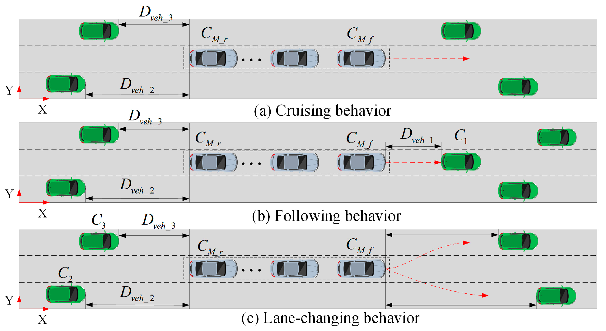
4.1. Vehicle Platoon Driving Decisions

When a vehicle platoon travels on the road, it must determine safe and cost-effective driving actions based on prevailing conditions and vehicle status, and subsequently create a reference trajectory. The decision-making procedure comprises two aspects: safety decisions and energy-saving decisions, with safety taking precedence. Only after ensuring safety are energy-efficient driving decisions made.

4.1.1. Safety Decision-Making

To ensure the vehicle platoon’s safe operation, we create a distance function linking the platoon and nearby vehicles, considering their states. Figure 3 illustrates the platoon’s typical driving scenario.

Vehicles need to obtain the critical collision distance for the surrounding vehicles by calculating the critical collision distance when changing lanes to avoid collisions. The minimum critical collision longitudinal safety distance can be determined by quadratic integration of the speed and initial speed difference between the vehicle platoon and the potentially colliding vehicles [41,42]. Assuming the driving state of the controlled vehicle formation and the surrounding vehicles remains constant for a brief period and that the vehicle formation’s integrity is maintained during the lane change, the safe distance between the vehicle formation and the surrounding vehicles can be calculated using the following equation:

$$\begin{array}{ll}MSS(C_{M\_f},C_1)=& \max \left\{{\int }_0^t{\int }_0^{\lambda }[a_{M\_f}(\tau )-a_1(\tau )]d\tau d\lambda \right.\\ & \left.+[v_{M\_f}(0)-v_1(0)]t\right\},\forall t\in [0,t_c]\end{array}$$

(9)

$$\begin{array}{ll}MSS(C_{(M\_r},C_2)=& \max \left\{{\int }_0^t{\int }_0^{\lambda }[a_{M\_r}(\tau )-a_2(\tau )]d\tau d\lambda \right.\\ & \left.+[v_{M\_r}(0)-v_2(0)]t\right\},\forall t\in [0,t_f]\end{array}$$

(10)

$$\begin{array}{ll}MSS(C_{(M\_r},C_3)=& \max \left\{{\int }_0^t{\int }_0^{\lambda }[a_{M\_r}(\tau )-a_3(\tau )]d\tau d\lambda \right.\\ & \left.+[v_{M\_r}(0)-v_3(0)]t\right\},\forall t\in [0,t_f]\end{array}$$

(11)

where $C_{M\_f}$ and $C_{M\_r}$ represent the lead vehicle and tail vehicle of the controlled vehicle platoon; $C_i(i=1,2,3\dots )$ represents surroundings vehicles, $D_{veh\_i}(i=1,2,3\dots )$ represents the actual longitudinal distance during the lane change; $a_{M\_f}$ and $v_{M\_f}$ represent the acceleration and speed of the leading vehicle of the controlled vehicle platoon; $a_{M\_r}$ and $v_{M\_r}$ represent the acceleration and velocity of the trailing vehicle of the controlled vehicle platoon; $a_i(i=1,2,3\dots )$ and $v_i(i=1,2,3\dots )$ represent the acceleration and velocity of $C_i(i=1,2,3\dots )$, respectively; $t_c$ is the collision time; and $t_f$ is the time required to change lanes and is determined in the next section.

The longitudinal safety distance model integrating the critical minimum longitudinal safety distance and vehicle execution response time is represented as follows:

$$d_{s,i}=\left\{\begin{array}{cc}MSS(C_M,C_i) ,& v_m<v_f\\ (v_M-v_f)t_{ttc}+MSS(C_M,C_i),& v_m\ge v_f\end{array}\right.$$

(12)

where $v_f$ represents the leading or trailing vehicle of the controlled vehicle $a_{M\_r}$ platoon, $v_f$ is the speed of the target vehicle, and $t_{ttc}$ is the vehicle execution response time.

$$DE{C}_{sef}=\left\{\begin{array}{cc}NO\_SEF& ,\hspace{1em}{D}_{veh\_i}<d_{s,i}\\ YES\_SEF& ,\hspace{1em}{D}_{veh\_i}\ge d_{s,i}\end{array}\right.$$

(13)

where $DE{C}_{sef}$ denotes the safety decision function, and $NO\_SEF$ and $YES\_SEF$ denote the potential safety behaviors unsatisfied and satisfied.

4.1.2. Economic Decision-Making

While a vehicle travels on the road, the driving state of the preceding vehicle impacts the host vehicle’s state, subsequently influencing the vehicle’s driving economy. Therefore, accurately predicting the speed of the preceding vehicle is crucial [43]. RBF neural networks are adept at handling nonlinear multiple-input/multiple-output problems in time-series prediction and can precisely predict the uncertainty of dynamic processes, such as speed changes [44]. Leveraging V2V and onboard sensors, this paper acquires the historical speed data of vehicles in each lane ahead and employs an RBF neural network to construct a speed prediction model to aid in lane change decision-making for the vehicle platoon.

This paper uses several combinations of standard driving cycles to create the training library, including LA92, JN1015, WLTP, US06, and HUDDS. These standard cycles represent a variety of scenarios in which vehicles are driven on urban and highway roads, and different working condition information is fully considered to ensure that the RBF neural network can adequately train and learn relevant features. The RBF neural network speed predictor’s prediction accuracy is tested using typical highway conditions (HWFET) and typical urban traffic conditions (INDIA_URBAN), and the prediction results are shown in Figure 4 and Figure 5. When the prediction time horizon is 5 s, the RMSE is 0.2571 and 0.2606 under urban mobility and highway conditions, respectively, and the prediction results are shown below. In most cases, the predicted speed can match the change rule of the actual speed, which, to a certain extent, reflects the driving speed characteristics of the vehicle in the future period.

One of the key factors influencing vehicle driving economy is the slow speed or significant speed fluctuation of the preceding vehicle, which necessitates frequent speed adjustments for the following vehicle, thereby increasing energy consumption. The established RBF speed prediction model forecasts the speed of the preceding vehicle and assesses its speed level and fluctuation based on historical and predicted speed data. An evaluation index reflecting energy consumption cost and speed fluctuation is developed based on the vehicle platoon’s economic cruising speed to decide whether the platoon should follow the preceding vehicle. The objective function for evaluating vehicle platoon lane changes can be expressed as follows:

$$J_{lc}={\omega }_e\cdot {\displaystyle \frac{{\displaystyle {\sum }_{i=0}^n{Q}_i}}{n}}+{\omega }_v\cdot \left|v_{\max }-v_{\min }\right|+{\omega }_a\cdot {{\displaystyle {\sum }_{i=0}^n\Delta v}}^2$$

(14)

where $J_{lc}$ is the lane change evaluation function; n represents the count of sample time points within the speed prediction interval; $v_{\max }$ and $v_{\min }$ are the maximum and minimum values of the speed in the prediction time domain, respectively, which are used to characterize the degree of speed change in the prediction time domain; $\Delta v$ is the amount of speed change in the predicted time domain; and ${\omega }_e$, ${\omega }_v$, and ${\omega }_a$ denote the weights of the energy cost, the degree of speed change, and the amount of speed change, respectively. Additionally, $Q_i$ is the predicted energy cost derived from speed predictions using the energy consumption model, with the economic cruising speed serving as the energy consumption evaluation index, which can be expressed as follows:

$$Q_i=\left\{\begin{array}{ll}Q(v_{eco})& v_i\ge v_{eco}\\ Q(v_i)& v_i<v_{eco}\end{array}\right.$$

(15)

Therefore, the lane change energy-saving decision can be constructed as follows:

$$DE{C}_{eco}=\left\{\begin{array}{ll}NO\_ECO& J_{lc\_t\arg e}<J_{lc\_host}-\epsilon \\ YES\_ECO& J_{lc\_t\arg e}\ge J_{lc\_host}-\epsilon \end{array}\right.$$

(16)

where $DE{C}_{eco}$ is the energy-saving decision function; $J_{lc\_t\arg e}$ and $J_{lc\_host}$ are the values of the lane-changing evaluation function for the target lane and the home lane, respectively; and $\epsilon$ is the lane-changing relaxation factor, which varies with the relative distances between the front vehicle in the target lane and the host vehicle.

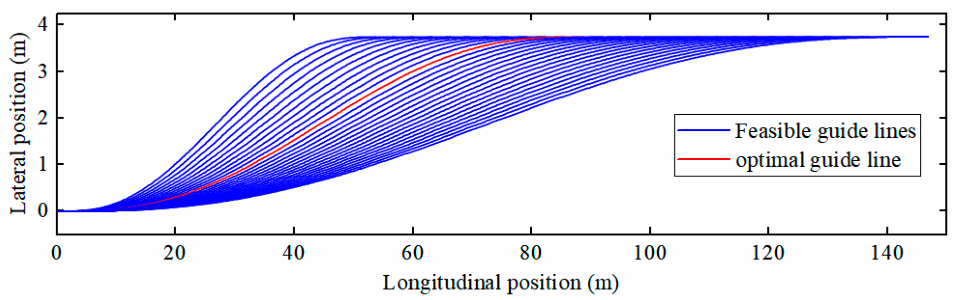
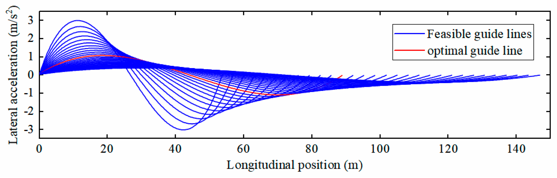
4.2. Vehicle Platoon Trajectory Generation

Geometry-based trajectory planning usually uses parameterized curves to describe the trajectory, which is intuitive and accurate and enables flexible control of the trajectory shape by adjusting the parameters of the curves. Compared with other complex trajectory planning methods, the parametric curve description is easily understood and implemented, and the computation volume is relatively small, which is suitable for real-time vehicle control systems. Therefore, in this paper, the fourth- and fifth-degree polynomials about time, t, are utilized to characterize the longitudinal and lateral movements, respectively, and the trajectory equations are as follows:

$$\left\{\begin{array}{c}x={\displaystyle \sum _{i=0}^4}{a}_i{t}^i\\ y={\displaystyle \sum _{i=0}^5}{b}_i{t}^i\end{array}\right.$$

(17)

where $x$ and $y$ are the longitudinal and lateral movements of the host vehicle at the moment $t$, $t\in [t_0,t_f]$; $t_0$ is the starting moment of the vehicle lane change; and $a_i$ and $b_i$ are the coefficients of the vehicle lane change trajectory equation, respectively.

Since the trajectory equation is a function of time, $t$, the longitudinal and transverse velocities, $v_x$ and $v_y$, and the longitudinal and lateral accelerations, $a_x$ and $a_y$, of the vehicle at each moment can be obtained by taking the first and second derivatives of the equation, and thus the boundary conditions corresponding to the lane-changing trajectory are as follows:

$$\left\{\begin{array}{l}x(t_0)=x_0,\dot{x}(t_0)=v_{x0},\ddot{x}(t_0)=a_{x0},\\ y(t_0)=y_0,\dot{y}(t_0)=v_{y0},\ddot{y}(t_0)=a_{y0},\\ \dot{x}(t_f)=v_{xf},\ddot{x}(t_f)=a_{xf},\\ y(t_f)=y_f,\dot{y}(t_f)=v_{yf},\ddot{y}(t_f)=a_{yf},\end{array}\right.$$

(18)

where $(x_0,v_{x0},a_{x0})$ are the motion state at the initial moment of the host vehicle lane change, and $(v_{xf},a_{xf})$ and $(y_f,v_{yf},a_{yf})$ are the motion state at the end of the host vehicle lane change.

Since the initial state $(x_0,v_{x0},a_{x0},y_0,v_{y0},a_{y0})$ and the lateral displacement, $y_f$, at the end of the lane change are known, we want the vehicle to be in a stable state with uniform speed as much as possible at the end of the lane change, and set the lateral velocity, $v_{yf}$ and the longitudinal and lateral accelerations, $a_{xf}$ and $a_{yf}$, at the end of the lane change to be 0. Therefore, the lane change trajectory problem is transformed into an optimization problem for solving $t_f$ and $v_{xf}$.

Based on the statistical analysis of human drivers’ lane-changing behavior, the time horizon of lane changing is set to $t_f\in [1.5,13.2]$, and $v_{xf}$ is the speed that the vehicle wishes to reach in the target lane at the end of the lane change. If no vehicle is in front of the target lane, $v_{xf}$ is set to the economic speed; otherwise, $v_{xf}$ is set to the speed of the vehicle in front.

Here, $v_e$ is the economic speed of the vehicle, and $v_F$ is the speed of the vehicle in front of the target lane.

To achieve the optimal lane-changing trajectory, this paper presents the lane-changing trajectory evaluation function, $J$, to optimize the lane-changing time, considering the vehicle’s safety, comfort, and driving efficiency. In order to simplify the calculation, the maximum lateral acceleration and lane-changing time in the vehicle driving process are taken as the optimization variables. Considering the dynamic constraints of the vehicle in the lane changing process, as well as to ensure the stability of the lane-changing process, the lateral velocity, $v_y$; the lateral acceleration, $a_y$; and the vehicle’s transverse angular velocity, $\phi$, need to be constrained, and the optimization function and constraints are as follows:

$$\min J(a_y,t_f)={\omega }_1{\displaystyle \frac{\left|a_{y\max }\right|}{a_{y\max }^{all}}}+{\omega }_2{\displaystyle \frac{t_f}{t_{f\max }}}$$

(19)

$$st.\left\{\begin{array}{l}{v}_{y\min }<v_y<v_{y\max }\\ a_{y\min }<a_y<a_{y\max }\\ {\phi }_{\min }<\phi <{\phi }_{\max }\end{array}\right.$$

(20)

where ${\omega }_1$ and ${\omega }_2$ are the weights occupied by each evaluation index; ${\omega }_1+{\omega }_2=1$. $a_{y\max }^{all}$ is the maximum lateral acceleration of the vehicle in the lane-changing trajectory; $a_{y\max }$ is the maximum lateral acceleration that the vehicle can achieve; and $t_{f\max }$ is the maximum lane-changing time required by the vehicle.

The MATLAB 2022b optimization function, fmincon, is used to optimally solve the multi-objective cost function, resulting in optimized lane change trajectories and lateral accelerations, as shown in Figure 6 and Figure 7.

Traditional lane change trajectory planning studies usually assume that the surrounding vehicles maintain a constant motion state. However, in case of unexpected conditions, such as emergency braking by the vehicle in front of the target lane, continuing to track the initial planning trajectory will lead to a significant increase in the probability of collision, thus constituting a potential safety hazard. To address this key issue, this study proposes a dynamic window-based lane change trajectory adjustment method, which is schematically shown in Figure 8. Through real-time sensing and motion prediction, the lane change trajectory is dynamically updated at regular intervals to improve driving safety in complex situations effectively.

5. Trajectory Tracking Control Based on MPC

5.1. Construction of Vehicle Kinematics Model

Trajectory tracking control is designed to swiftly and precisely follow a reference trajectory. In this paper, a linear two-degrees-of-freedom vehicle kinematic model is employed to verify vehicle alignment control.

As shown in the Figure 9, in the inertial system XOY, (x,y) represents the coordinates of the center of the rear axle of the vehicle, $\phi$ is the heading angle, $\delta$ is the front wheel angle of rotation, $v$ is the velocity of the midpoint of the rear axle, and $l$ is the wheelbase.

The vehicle kinematic model can be expressed by the following equation:

$${\left.\dot{\chi }=\left[\begin{array}{ccc}\dot{x}& \dot{y}& \dot{\phi }\end{array}\right.\right]}^T={\left[\begin{array}{ccc}\cos \phi & \sin \phi & {\displaystyle \frac{1}{l}}\tan \delta \end{array}\right]}^{T}v$$

(21)

The longitudinal position, lateral position, and orientation angle are used as system state quantities to obtain the discrete vehicle system as follows:

$$\chi (k+1)=\left[\begin{array}{c}x(k+1)\\ y(k+1)\\ \phi (k+1)\end{array}\right]=\left[\begin{array}{c}x(k)+\mathsf{\Delta }t\cdot v(k)\cos \left(\phi (k)\right)\\ y(k)+\mathsf{\Delta }t\cdot v(k)\sin \left(\phi (k)\right)\\ \phi (k)+\mathsf{\Delta }t\cdot v(k)/l\cdot \tan \left(\delta (k)\right)\end{array}\right]$$

(22)

where $\Delta t$ is the discrete time step, and $x(k+1)$ denotes the system state the (k + 1) moment. In order to constrain the control increments in the MPC, Equation (22) should be transformed as follows:

$$\left.\xi \left(k+1\right)=\left[\begin{array}{c}x(k+1)\\ y(k+1)\\ \phi (k+1)\\ v(k+1)\\ \delta (k+1)\end{array}\right.\right]=\left[\begin{array}{c}x(k)+\mathsf{\Delta }t\cdot v(k)\cos \left(\phi (k)\right)\\ y(k)+\mathsf{\Delta }t\cdot v(k)\sin \left(\phi (k)\right)\\ \phi (k)+\mathsf{\Delta }t\cdot v(k)/l\cdot \tan \left(\delta (k)\right)\\ v(k)+\mathsf{\Delta }v(k+1)\\ \delta (k)+\mathsf{\Delta }\delta (k+1)\end{array}\right]$$

(23)

where $\mathsf{\Delta }u=u(k)-u(k-1)$ denotes the control increment, ${[\mathsf{\Delta }v(k),\mathsf{\Delta }\delta (k)]}^T$, which represents the acceleration and front wheel steering angle increment of the vehicle at moment k, respectively.

5.2. Objective Function and Constraint Setting for MPC

In cooperative control systems, a cost function must be established in line with the control objective to guarantee the controller’s effectiveness. This cost function should reflect how well the vehicle tracks the desired trajectory and speed, and it should also ensure a comfortable ride for the driver. The cost function comprises a weighted combination of tracking error and control increment. In addition, the MPC controller should also consider the relevant dynamics constraints of the actuator, where the primary considerations are the speed of the vehicle, $v$; acceleration, $a$; and the limit value of the front wheel angle, $\delta$. The cost function and constraints can be expressed in the following equation:

$$\begin{array}{ll}\min J_{leader}\left(k\right)=& {\displaystyle \sum _{i=1}^{Np}}{w}_x{‖e_{x1}\left(i\right)‖}^2+{\displaystyle \sum _{i=1}^{Np}}{w}_y{‖e_{y1}\left(i\right)‖}^2\\ & +{\displaystyle \sum _{i=1}^{Np}}{w}_v{‖e_{v1}\left(i\right)‖}^2+{\displaystyle \sum _{i=1}^{Nc-1}}{w}_u{‖\Delta u(k+1|k)‖}^2\end{array}$$

(24)

$$\begin{array}{ll}\min J_{follower}\left(k\right)=& {\displaystyle \sum _{i=1}^{Np}}{w}_x{‖e_{x2}\left(i\right)-S‖}^2+{\displaystyle \sum _{i=1}^{Np}}{w}_y{‖e_{y2}\left(i\right)‖}^2\\ & +{\displaystyle \sum _{i=1}^{Np}}{w}_v{‖e_{v2}\left(i\right)‖}^2+{\displaystyle \sum _{i=1}^{Nc-1}}{w}_u{‖\Delta u(k+1|k)‖}^2\end{array}$$

(25)

$$s.t \left\{\begin{array}{l}0\le v\le v_{\max }\\ a_{\min }\le a\le a_{\max }\\ -{\delta }_{\max }\le \delta \le {\delta }_{\max }\\ -{\dot{\delta }}_{\min }\le \dot{\delta }\le {\dot{\delta }}_{\max }\end{array}\right.$$

(26)

where $J_{leader}$ and $J_{follower}$ are the cost functions for the lead and follower vehicles within the platoon, respectively; $e_{x1}\left(i\right)$, $e_{y1}\left(i\right)$, and $e_{v1}\left(i\right)$ are the longitudinal, lateral, and velocity errors of the predicted trajectory of the leading vehicle with respect to the reference trajectory in the prediction time domain, respectively; $e_{x2}\left(i\right)$, $e_{y2}\left(i\right)$, and $e_{v2}\left(i\right)$ are the longitudinal, lateral, and velocity discrepancies between the follower vehicle and the anticipated path of the preceding vehicle over the prediction horizon, respectively $w_x$, $w_y$, $w_v$, and $w_u$ are different weighting factors of MPC controller different weight factors for optimization; $N_p$ and $N_c$ are the prediction step size and control step size; $\Delta u(k+1|k)$ denotes the control increment to be minimized; and $S$ is the vehicle spacing between two neighboring vehicles in the platoon.

6. Vehicle Cooperative System Modeling Based on Hybrid Automata

Vehicle cooperative control can be viewed as a combination of continuous vehicle motion control and discrete maneuvering transition rules, requiring a cooperative mechanism for their flexible transition and operation. Hybrid automata, a formal tool for modeling time-ordered dynamical systems, combines finite state machines and continuous state variables to describe complex system behaviors, including discrete and continuous behaviors. Therefore, this section employs the hybrid automaton framework to construct the collaborative system, facilitating the coordination and transitions between platoon mergers and splits.

Construct the tuple, $H$, for the collaborative control system according to the syntax of the hybrid automata:

$$H=<Q,Var,Con,Event,Edge,Act,Inv,Init>$$

(27)

where $Q=\{Q_1,Q_2\}$ represents a limited collection of control modes for the cooperative system; $Q_1$ represents a vehicle in a leading state or a single-vehicle cruising state; $Q_2$ represents a vehicle in a following state; Var and Con represent the control vectors of the system, comprising acceleration and steering angle; $Event=\{\mathrm{MERGE},\mathrm{SPLIT}\}$ represents the set of events for the system transitions, consisting of vehicle merging and splitting; and $Edge,Act,Inv,Init$ represent the discrete maneuvering successive control subsystems, operation constraints, initial conditions, and transition processes.

6.1. Vehicle and Environmental Status Definitions

To make driving behavior decisions based on the vehicle’s current status and the surrounding environment, we define a set of vehicle attributes to depict the controlled vehicle’s condition and the sensed status of nearby vehicles.

As shown in Figure 10, the surrounding vehicles are categorized into communicable vehicles equipped with V2V systems and obstacle vehicles without communication capabilities, and the collected information is categorized into information collected by onboard sensors and information acquired by V2V.

$$\begin{array}{cc}Car=& [ID,Carparameter,CarState,\hfill \\ & Platoondata,Sensordata,Wirelessdata]\end{array}$$

(28)

$$ObCar=[ID,CarState,Sensordata]$$

(29)

where $ID$ represents the vehicle identifier on the road, which is equivalent to the vehicle’s license plate; $Carparameter$ is the vehicle’s parameter information, including the vehicle’s mass, transmission system parameters, wind resistance coefficient, etc.; $CarState$ is the current motion state of the vehicle, including the position, speed, acceleration, the angle of the front wheels at the current moment, etc.; and $Platoondata$ represents the parameters related to the vehicle platooning, including the platoon number, platoon length, and willingness of formations.

$Sensordata$ is the surrounding vehicle information sensed by the vehicle sensor, which contains only the vehicle’s motion state information and has a specific distance limitation. $Wirelessdata$ is the vehicle information of the road section acquired by the V2V communication, which contains the vehicle’s motion state information, the vehicle’s parameter information, platoon information, and all other information.

6.2. Event Triggering Rules

Merging and splitting of platoons are essential issues in cooperative control systems. This section details how to model these two events in a hybrid automaton. Figure 11 depicts the modeling process of merging and splitting of platoons.

Merge event: Any vehicle within the detection range of the platoon’s front and rear is deemed a potential member for integration into the platoon. The platoon under control constantly tracks the movement status of these potential members. If such a member satisfies the specified speed and spacing requirements and consents to join the platoon, a merge signal is activated to incorporate this member into the platoon.

Split event: During the splitting event, the controlled vehicle platoon continuously monitors the motion state within the platoon and changes in the surrounding environment. When the platoon is no longer suitable for following, or the vehicles in the platoon have the need to leave the platoon voluntarily, a separation signal will be activated, the target vehicle will be removed from the current platoon, and its motion state will be adjusted to detach from the platoon.

Table 2. Change in discrete states before and after platoon merging.

VehID	Transition	PltnEn	PlatoonID	PrecedID	PltnNum	PltnLength	Manv
PV-1	Before	1	Pltn-1	0	1	2	Cruising
	After	1	Pltn-1	0	1	3	Cruising
PV-2	Before	1	Pltn-1	PV-1	2	2	Platooning
	After	1	Pltn-1	PV-1	2	3	Platooning
PV-3	Before	1	Pltn-3	0	1	3	Cruising
	After	1	Pltn-3	0	1	2	Cruising
PV-4	Before	1	Pltn-3	PV-3	2	3	Platooning
	After	1	Pltn-3	PV-3	2	2	Platooning
PV-5	Before	1	Pltn-3	PV-3	3	3	Platooning
	After	1	Pltn-1	PV-1	3	3	Platooning

provides details on the changes in vehicle motion states prior to and following the split.

7. Simulation Test

7.1. Platoon Stability Verification

In real V2X communication scenarios, non-ideal factors such as channel noise and time-varying delay can seriously affect the robustness of the system. To enhance the practical applicability of the model, we establish a state compensation mechanism: when the system detects successive packet losses or communication delays, we reconstruct the current state using historical state data and estimate the current state in conjunction with model predictions. In order to model accurate communication lag data, we build simulation experiments using measurements from the literature to verify the string stability and internal stability of the platoon in performing various operations [45,46,47].

7.1.1. String Stability

A platoon of five self-driving cars is traveling on the road, and the input communication time-lag noise is shown in Figure 12, and a step response is applied to the acceleration of the pilot car. Figure 13a–d show the control effects with and for the state compensation mechanism, respectively, from which it can be seen that the model predictive controller with the state compensation mechanism effectively reduces the control perturbation caused by the communication time lag and ensures the string stability of the platoon while traveling.

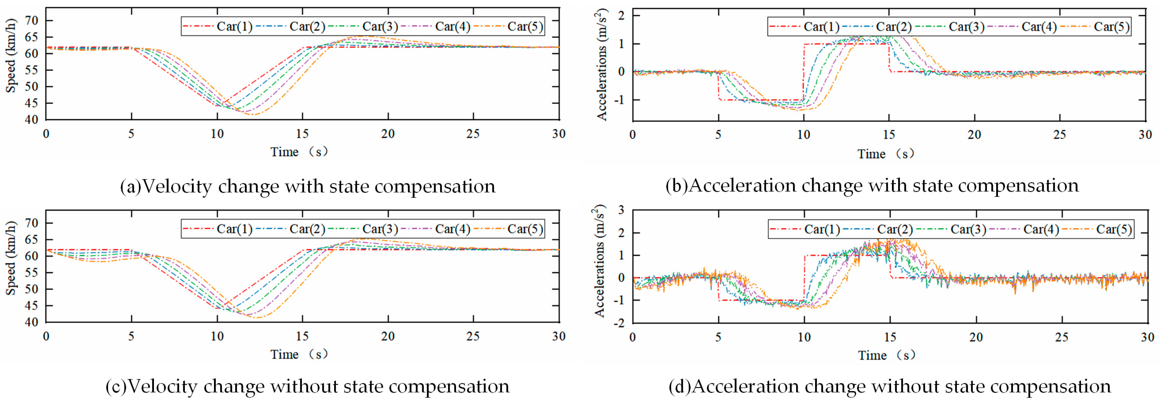
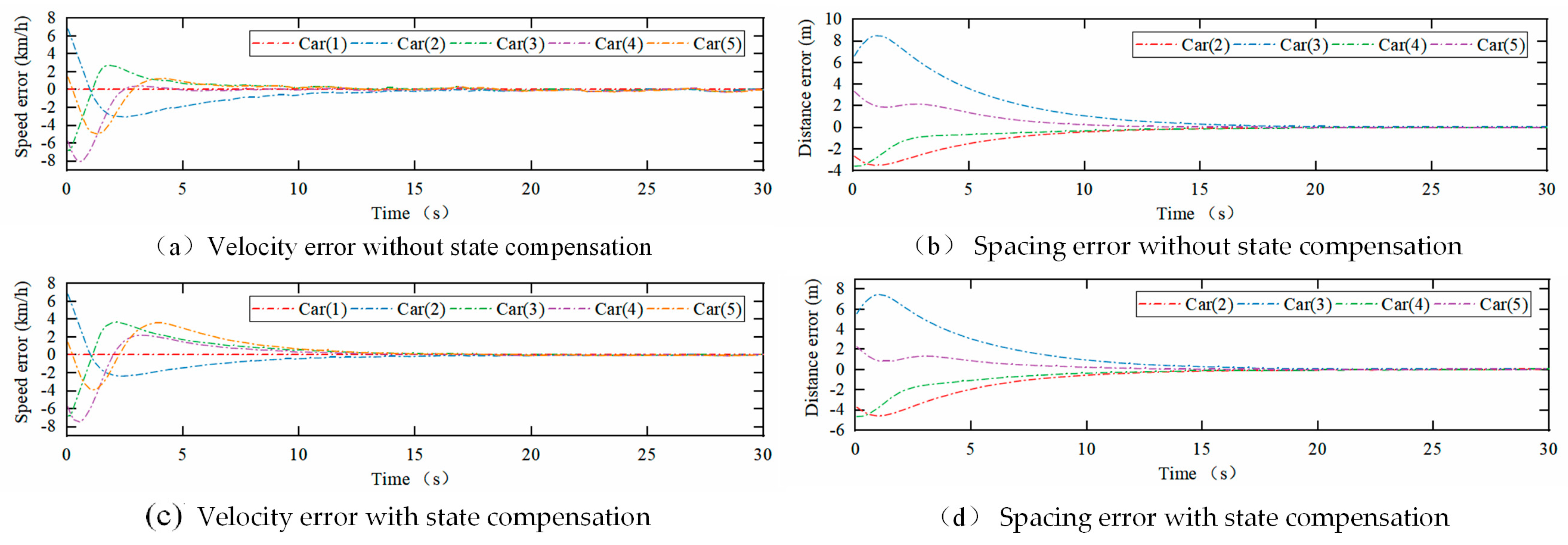
7.1.2. Internal Stability

In order to verify the internal stability of the platoon, the leading vehicle was set to travel at a constant speed, and the distance, speed, and acceleration errors were set so that the platoon was in an unstable state at the beginning. Figure 14a,b show the changes in speed error and spacing error without setting the state compensation mechanism, and Figure 14c,d show the changes in speed error and spacing error with setting the state compensation mechanism. From the simulation results, it can be seen that the MPC controller with the compensation mechanism set can effectively reduce the fluctuation of the fleet’s spacing adjustment process, which improves the system’s robustness to a certain extent.

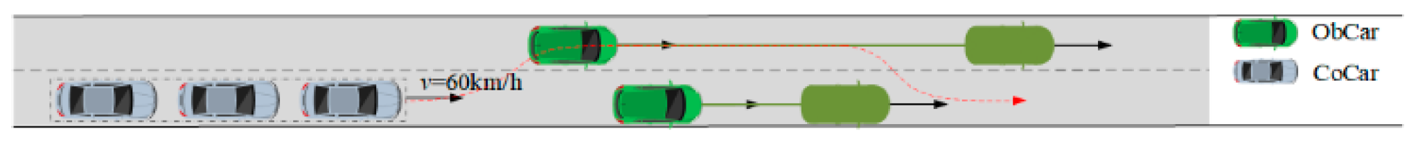
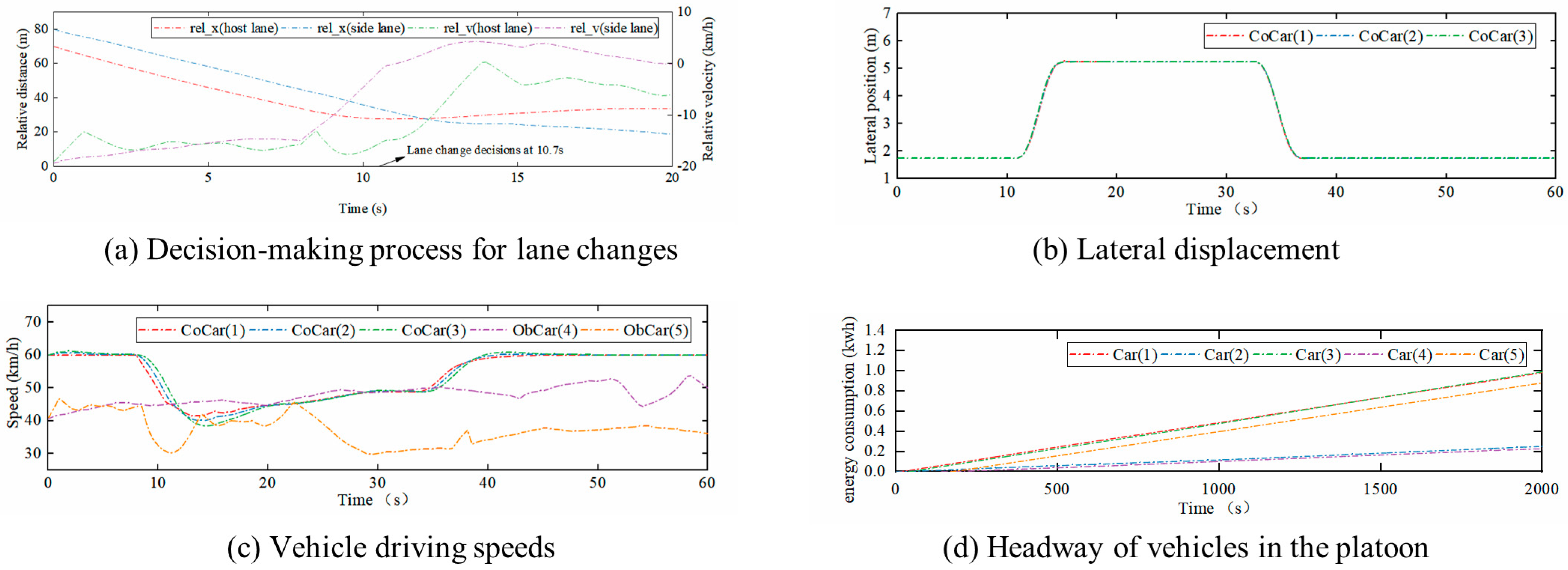
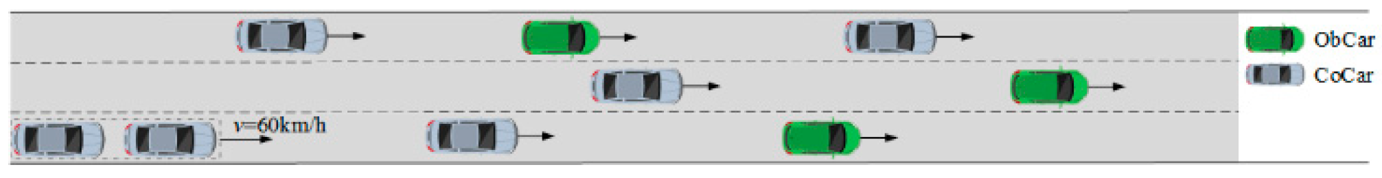
7.2. Vehicle Platoon Lane Change Verification

To verify the effectiveness of vehicle platoon lane changing, the test environment is constructed by extracting the actual speed information of the surrounding vehicles over a certain period from the dataset [48]. The average computation time for each time-step optimization problem is 0.0102 s. This was achieved using a personal computer equipped with an Intel Core i5-12400 CPU @ 2.50 GHz, 16 GB RAM, and 512 GB SSD (Intel Corporation, Santa Clara, CA, USA). Given that the step size is 0.02 s, the optimization problem can be solved in real time.

As shown in Figure 15, the platoon travels on the road at an economical speed of 60 km/h. There are obstacle vehicles in both the primary and side lanes, and the platoon needs to decide on changing lanes according to the status of the vehicles in front of different lanes. From Figure 16a, it can be seen that at the beginning of the two lanes, the speed level of the vehicle in front of the platoon is comparable. The platoon did not choose to carry out the lane change; it chose to decelerate to change lanes to maintain a safe distance from the vehicle in front of the platoon until 10.7 s. The central lane is that of the vehicle in front of the apparent deceleration tendency, and at this time, having the conditions of safe change into the side lane, the platoon choose to carry out the lane change. From Figure 16b–d, it can be seen that the platoon always keeps driving closely during the driving process, and the spacing within the platoon is also kept within a reasonable range.

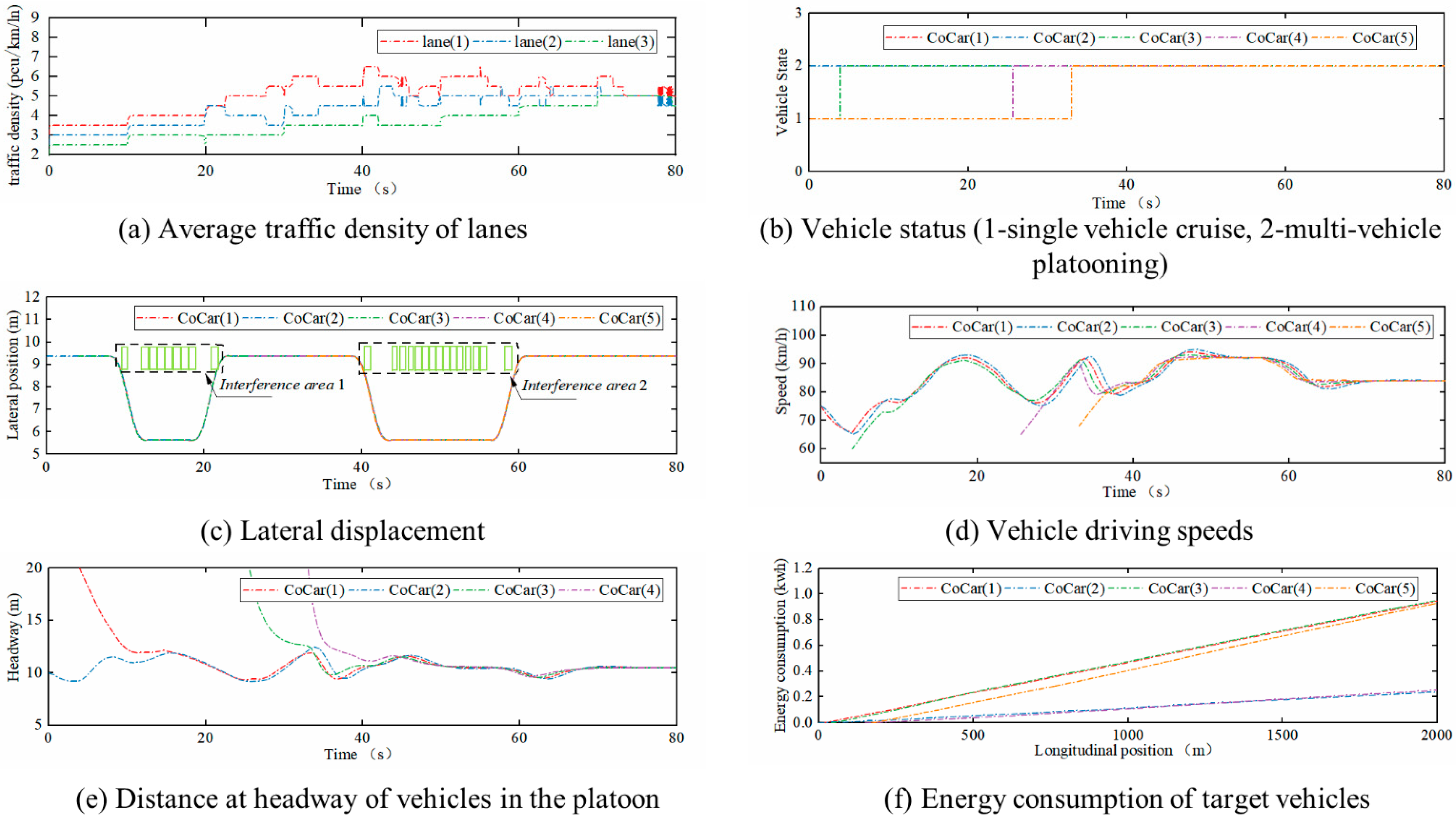
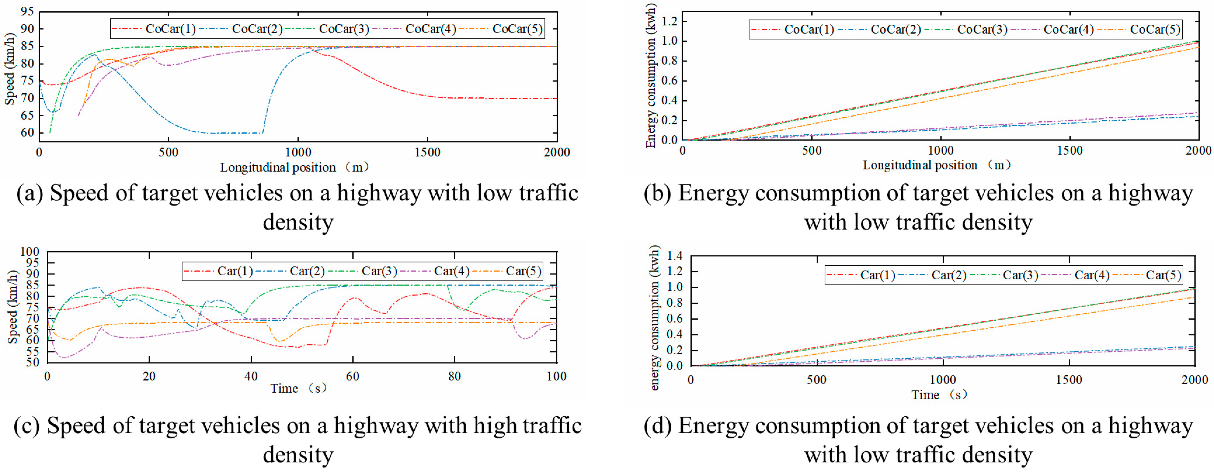
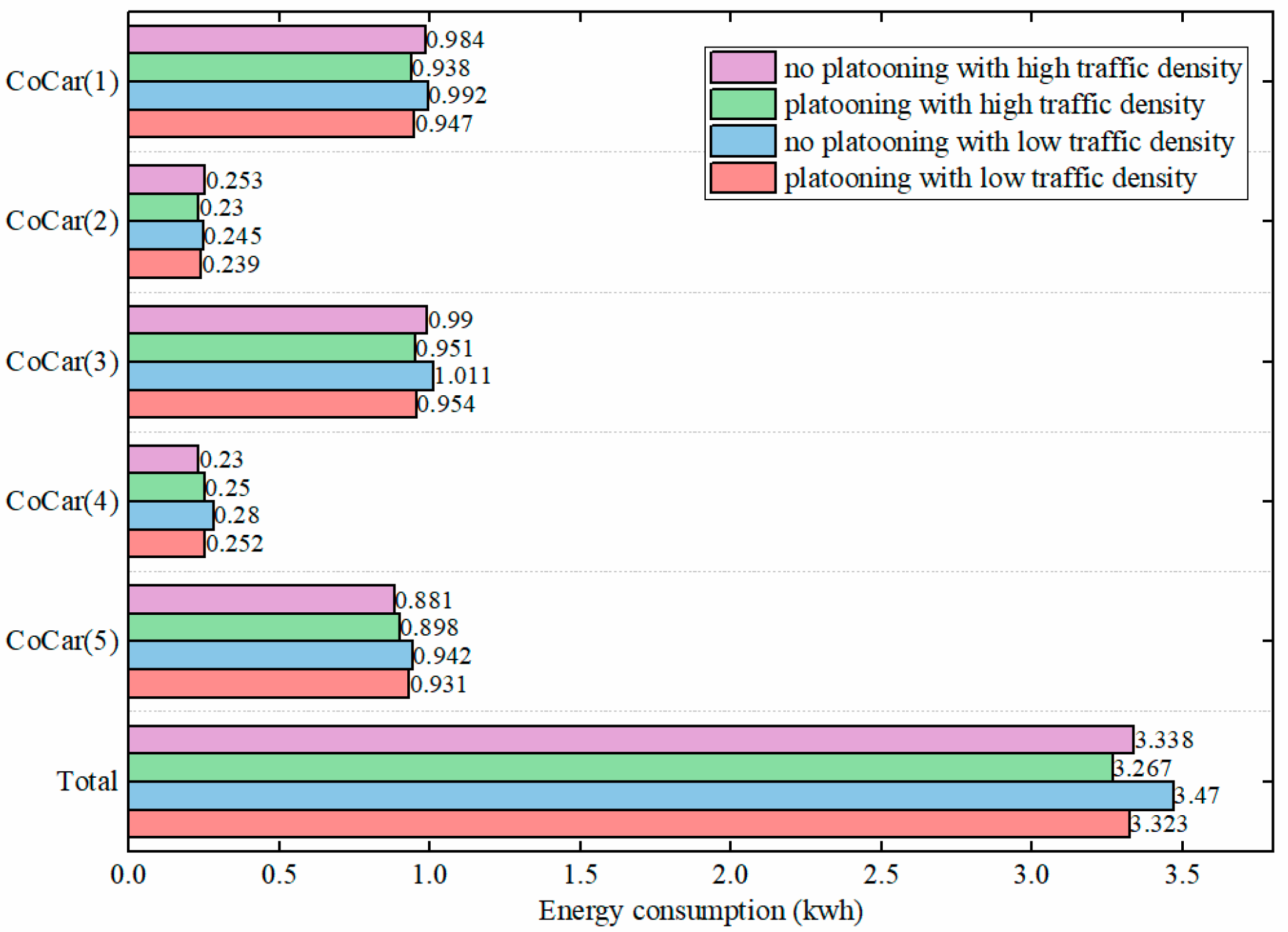
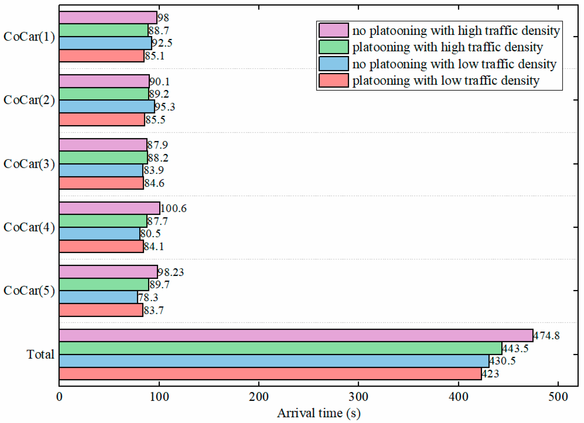
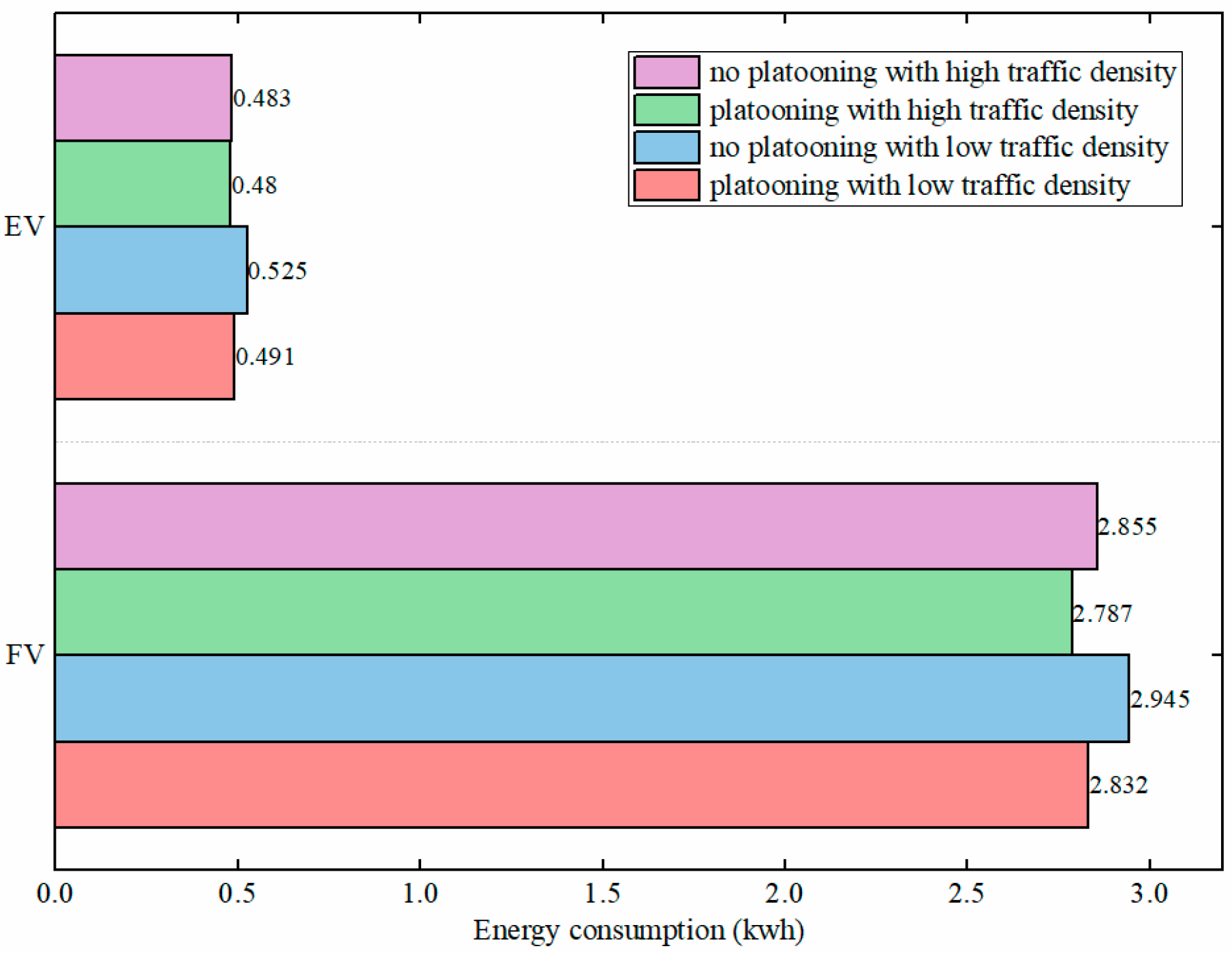
7.3. Energy Efficiency Verification

In order to verify the effectiveness and applicability of the proposed algorithm, this paper evaluates its energy-saving performance by simulating it in the constructed highway scenario, and the simulation parameters are set as shown in

Table 3. Simulation Parameters.

	Initial Number of Vehicles	Vehicle Generation Time	Speed Range
Low traffic density	20	10 s	60–90 km/h
High traffic density	60	3 s	60–90 km/h

. The Intelligent Driver Model (IDM) simulates the driving behavior of vehicles operating independently, while a probabilistic lane-changing model replicates lane changes when vehicles approach preceding vehicles [49]. To investigate energy savings across varying traffic densities, vehicles are systematically introduced at road entrances at set intervals, and traffic density is regulated by adjusting these intervals. There are two main methods for vehicle platoon merging: when the target vehicle and the platoon share the same lane, the inter-vehicle distance is adjusted for direct merging; when they are in different lanes, the target vehicle is programmed to join the platoon from the rear to minimize impact on the platoon’s overall driving efficiency.

As depicted in Figure 17, a standard three-lane highway in one direction is constructed, with the speed limit established in accordance with the specifications of China’s national road standards. Each lane is 3.75 m wide, and the total length of the road segment is 2000 m. The road gradient is relatively smooth because of the gradient of the highway, and because the slope of the highway is relatively gentle, this paper does not consider the road gradient for the time being. In order to simulate the driving environment of vehicles in different traffic densities, different numbers of vehicles are initialized. At the same time, three vehicles are initialized at the entrance of the road at regular intervals to simulate the dynamic driving environment of the highway.

As shown in Figure 18a, the traffic density is set to be a low-traffic-density environment not exceeding 7 pcu/km/ln. The platoon, composed of two vehicles, starts to drive on the road at 75 km/h. As shown in Figure 18b, the vehicle in front of this lane joins the platoon from the front at 3.9 s, 25.6 s, and 33 s, respectively, and the platoon chooses to change lanes in the face of the obstacle vehicle in front of the platoon at 7.9 s and 38.8 s. Since the economic speed of the platoon is below 90 km/h, to satisfy the highway lane’s speed limit, the platoon needs to accelerate to overtake the vehicle in front of it and then change back to this lane. From Figure 18c,e, we can see that the whole process meets the requirements of the road speed limit, and the queue spacing is also kept within a reasonable range. Meanwhile, Figure 18c,d show that the platoon is less affected by the surrounding vehicles by actively changing lanes to follow the economic cruising speed.

As shown in Figure 19a, the traffic density is set to a high traffic density environment of 20 pcu/km/ln. As shown in Figure 19b, at 3.9 s and 30 s, the vehicle ahead in this lane joins the platoon from the front, and at 69.5 s, the vehicle from the adjacent lane merges into the platoon from the rear. At 7.3 s, confronted with the obstacle vehicle ahead, the platoon opts for a lane change. Subsequently, due to the hindrance posed by the surrounding vehicle, the vehicle decides to follow the one ahead. As illustrated in Figure 19c,d, to preserve the platoon’s integrity in dense traffic, it becomes challenging for the platoon to adhere to the economic cruising speed through frequent lane changes. Therefore, it chooses to follow the vehicle ahead, which is more influenced by the surrounding vehicles.

In order to evaluate the energy consumption performance of vehicles traveling in formation, the speed and energy consumption curves of vehicles traveling discretely in different traffic densities are shown in Figure 20. As shown in Figure 21 and Figure 22, for different traffic densities on the highway, the total energy consumption of the target vehicles is reduced by 2.13% and 4.24%, respectively, without increasing the travel time, even though the energy consumption of individual vehicles has increased. Therefore, the proposed strategy reduces the speed fluctuations on the highway to a certain extent, decreases the air resistance, and thus reduces the energy consumption of vehicles during driving. Figure 23 compares vehicles with different energy consumption characteristics. Regarding the energy-saving rate, the percentages of energy consumption reduction for fuel vehicles and electric vehicles are roughly the same, which are 3.12% and 3.67%, respectively. In terms of the total amount of energy consumption reduction, due to their energy consumption characteristics, the energy consumption reduction of fuel vehicles is approximately five times that of electric vehicles. In addition, in order to improve the reliability of the experimental results further, we conducted 10 simulations under different traffic densities. The average energy-saving rate and the standard deviation are shown in

Table 4. Average Energy Saving Rate and Standard Deviation Data.

	Average Energy Efficiency Rate	Standards Deviation
Low traffic density	2.86%	0.39%
High traffic density	3.25%	0.31%

. The results show that the energy-saving cooperative driving strategy proposed in this paper can effectively combine the vehicles driving discretely on the road into platoons and effectively reduce driving energy consumption.

8. Conclusions

In this paper, we propose a vehicle eco-co-driving system considering energy consumption characteristics that realizes the cooperative operation of vehicle formations, speed planning, and vehicle control. Firstly, a vehicle cooperative driving architecture was designed based on hybrid automata to establish the maneuver rules for vehicle merging and disbanding. Then, the energy consumption model was established and based on the energy consumption characteristics of different vehicles to obtain the optimal cruising speed of the vehicle platoon, provide economical lane change decision in case of encountering the vehicle ahead, and optimize the lane change trajectory. For the control problems of leading and following vehicles in the platoon, different control objectives were used as the cost function to control them, respectively. Finally, a three-lane highway scenario in the same direction was established, and the algorithms were tested by setting up environmental vehicles. The results show that the proposed vehicle ecological cooperative driving system can flexibly complete the formation merging operation, and the controller can ensure the stability of the vehicle platoon during the driving process. Vehicle merging and speed planning reduce the speed fluctuation in the road environment to a certain extent and improve the economy of the vehicle driving process. However, the shortcoming is that the lane-changing strategy in this paper is implemented based on guaranteeing platoon integrity, and the optimal timing of lane-changing may be missed in the case of high traffic density.

Therefore, in our future work, we will consider the long-term dynamic evolution of platooning on high-speed roads, and develop an energy consumption model considering battery degradation to study more complex energy optimization techniques for vehicle platoon [50]. We will further investigate how to implement vehicle splitting, merging, and lane-changing strategies based on road traffic density to adapt to the dynamically changing traffic environment through artificial intelligence methods such as reinforcement learning. At the same time, it is necessary to establish road scenarios considering road curvature, slope, and road surface adhesion coefficient based on real high-speed road data, validate the algorithms by using high-precision vehicle dynamics models, and conduct real road tests to further verify the experimental results.

References

1. Zahoor, A.; Mehr, F.; Mao, G.; Yu, Y.; Sápi, A. The carbon neutrality feasibility of worldwide and in China’s transportation sector by E-car and renewable energy sources before 2060. J. Energy Storage 2023, 61, 106696. [Google Scholar] [CrossRef]
2. Rehman, F.U.; Islam, M.; Miao, Q. Environmental sustainability via green transportation: A case of the top 10 energy transition nations. Transp. Policy 2023, 137, 32–44. [Google Scholar] [CrossRef]
3. Matin, A.; Dia, H. Impacts of Connected and Automated Vehicles on Road Safety and Efficiency: A Systematic Literature Review. IEEE Trans. Intell. Transp. Syst. 2023, 24, 2705–2736. [Google Scholar] [CrossRef]
4. Wang, B.; Su, R. A Distributed Platoon Control Framework for Connected Automated Vehicles in an Urban Traffic Network. IEEE Trans. Control Netw. Syst. 2022, 9, 1717–1730. [Google Scholar] [CrossRef]
5. Pi, D.; Xue, P.; Wang, W.; Xie, B.; Wang, H.; Wang, X.; Yin, G. Automotive platoon energy-saving: A review. Renew. Sustain. Energy Rev. 2023, 179, 113268. [Google Scholar] [CrossRef]
6. Hussein, A.A.; Rakha, H.A. Vehicle Platooning Impact on Drag Coefficients and Energy/Fuel Saving Implications. IEEE Trans. Veh. Technol. 2022, 71, 1199–1208. [Google Scholar] [CrossRef]
7. Stegner, E.; Ward, J.; Siefert, J.; Hoffman, M.; Bevly, D.M. Experimental Fuel Consumption Results from a Heterogeneous Four-Truck Platoon; SAE Technical Paper: Warrendale, PA, USA, 2021. [Google Scholar] [CrossRef]
8. Zhai, C.; Luo, F.; Liu, Y.; Chen, Z. Ecological Cooperative Look-Ahead Control for Automated Vehicles Travelling on Freeways with Varying Slopes. IEEE Trans. Veh. Technol. 2019, 68, 1208–1221. [Google Scholar] [CrossRef]
9. Jia, Y.; Nie, Z.; Wang, W.; Lian, Y.; Guerrero, J.M.; Outbib, R. Eco-driving policy for connected and automated fuel cell hybrid vehicles platoon in dynamic traffic scenarios. Int. J. Hydrogen Energy 2023, 48, 18816–18834. [Google Scholar] [CrossRef]
10. Ma, F.; Yang, Y.; Wang, J.; Li, X.; Wu, G.; Zhao, Y.; Wu, L.; Aksun-Guvenc, B.; Guvenc, L. Eco-driving-based cooperative adaptive cruise control of connected vehicles platoon at signalized intersections. Transp. Res. Part D Transp. Environ. 2021, 92, 102746. [Google Scholar] [CrossRef]
11. Wu, S.; Chen, Z.; Shen, S.; Shen, J.; Guo, F.; Liu, Y.; Zhang, Y. Hierarchical cooperative eco-driving control for connected autonomous vehicle platoon at signalized intersections. IET Intell. Transp. Syst. 2023, 17, 1560–1574. [Google Scholar] [CrossRef]
12. Liu, H.; Yan, S.; Shen, Y.; Li, C.; Zhang, Y.; Hussain, F. Model predictive control system based on direct yaw moment control for 4WID self-steering agriculture vehicle. Int. J. Agric. Biol. Eng. 2021, 14, 175–181. [Google Scholar] [CrossRef]
13. Su, Z.; Chen, P. Cooperative Eco-driving Controller for Battery Electric Vehicle Platooning. IFAC-Pap. 2022, 55, 205–210. [Google Scholar] [CrossRef]
14. Lacombe, R.; Gros, S.; Murgovski, N.; Kulcsár, B. Distributed Eco-Driving Control of a Platoon of Electric Vehicles Through Riccati Recursion. IEEE Trans. Intell. Transp. Syst. 2023, 24, 3048–3063. [Google Scholar] [CrossRef]
15. Hu, M.; Li, C.; Bian, Y.; Zhang, H.; Qin, Z.; Xu, B. Fuel Economy-Oriented Vehicle Platoon Control Using Economic Model Predictive Control. IEEE Trans. Intell. Transp. Syst. 2022, 23, 20836–20849. [Google Scholar] [CrossRef]
16. Zhu, Z.; Zeng, L.; Chen, L.; Zou, R.; Cai, Y. Fuzzy Adaptive Energy Management Strategy for a Hybrid Agricultural Tractor Equipped with HMCVT. Agriculture 2022, 12, 1986. [Google Scholar] [CrossRef]
17. Zhu, Z.; Yang, Y.; Wang, D.; Cai, Y.; Lai, L. Energy Saving Performance of Agricultural Tractor Equipped with Mechanic-Electronic-Hydraulic Powertrain System. Agriculture 2022, 12, 436. [Google Scholar] [CrossRef]
18. Li, A.; Xu, Z.; Li, W.; Chen, Y.; Pan, Y. Urban signalized intersection traffic state prediction: A spatial–temporal graph model integrating the cell transmission model and transformer. Appl. Sci. 2025, 15, 2377. [Google Scholar] [CrossRef]
19. Ala, M.V.; Yang, H.; Rakha, H. Modeling Evaluation of Eco–Cooperative Adaptive Cruise Control in Vicinity of Signalized Intersections. Transp. Res. Rec. J. Transp. Res. Board 2016, 2559, 108–119. [Google Scholar] [CrossRef]
20. Zhai, C.; Luo, F.; Liu, Y. Cooperative Power Split Optimization for a Group of Intelligent Electric Vehicles Travelling on a Highway with Varying Slopes. IEEE Trans. Intell. Transp. Syst. 2022, 23, 4993–5005. [Google Scholar] [CrossRef]
21. Jia, C.; Liu, W.; He, H.; Chau, K. Deep reinforcement learning-based energy management strategy for fuel cell buses integrating future road information and cabin comfort control. Energy Convers. Manag. 2024, 321, 119032. [Google Scholar] [CrossRef]
22. Jia, C.; Zhou, J.; He, H.; Li, J.; Wei, Z.; Li, K. Health-conscious deep reinforcement learning energy management for fuel cell buses integrating environmental and look-ahead road information. Energy 2024, 290, 130146. [Google Scholar] [CrossRef]
23. Li, K.; Zhou, J.; Jia, C.; Yi, F.; Zhang, C. Energy sources durability energy management for fuel cell hybrid electric bus based on deep reinforcement learning considering future terrain information. Int. J. Hydrogen Energy 2024, 52, 821–833. [Google Scholar] [CrossRef]
24. Zhang, H.; Chen, J.; Zhu, C.; Zhang, H. Deep Learning-Based Energy-Efficient Spacing Policy and Platooning Control Co-Design for Connected and Automated Vehicles on Inclined Roads. IEEE Trans. Veh. Technol. 2024, 73, 14486–14498. [Google Scholar] [CrossRef]
25. Wang, P.; Wang, X.; Ye, R.; Sun, Y.; Liu, C.; Zhang, J. Eco-driving-based mixed vehicular platoon control model for successive signalized intersections. Phys. A Stat. Mech. Its Appl. 2024, 639, 129641. [Google Scholar] [CrossRef]
26. Jiang, X.; Zhang, J.; Shi, X.; Cheng, J. Learning the Policy for Mixed Electric Platoon Control of Automated and Human-Driven Vehicles at Signalized Intersection: A Random Search Approach. IEEE Trans. Intell. Transp. Syst. 2023, 24, 5131–5143. [Google Scholar] [CrossRef]
27. Ma, Y.; Li, Z.; Malekian, R.; Zheng, S.; Sotelo, M.A. A Novel Multimode Hybrid Control Method for Cooperative Driving of an Automated Vehicle Platoon. IEEE Internet Things J. 2021, 8, 5822–5838. [Google Scholar] [CrossRef]
28. He, X.; Wu, X. Eco-driving advisory strategies for a platoon of mixed gasoline and electric vehicles in a connected vehicle system. Transp. Res. Part D Transp. Environ. 2018, 63, 907–922. [Google Scholar] [CrossRef]
29. Bichiou, Y.; Rakha, H. Vehicle Platooning: An Energy Consumption Perspective. In Proceedings of the 2020 IEEE 23rd International Conference on Intelligent Transportation Systems (ITSC), Rhodes, Greece, 20–23 September 2020; pp. 1–6. [Google Scholar] [CrossRef]
30. Yang, J.; Zhao, D.; Lan, J.; Xue, S.; Zhao, W.; Tian, D.; Zhou, Q.; Song, K. Eco-Driving of General Mixed Platoons with CAVs and HDVs. IEEE Trans. Intell. Veh. 2023, 8, 1190–1203. [Google Scholar] [CrossRef]
31. Wang, S.; Li, Z.; Wang, B.; Li, M. Collision Avoidance Motion Planning for Connected and Automated Vehicle Platoon Merging and Splitting with a Hybrid Automaton Architecture. IEEE Trans. Intell. Transp. Syst. 2024, 25, 1445–1464. [Google Scholar] [CrossRef]
32. Wang, Y.; Wang, L.; Guo, J.; Papamichail, I.; Papageorgiou, M.; Wang, F.-Y.; Bertini, R.; Hua, W.; Yang, Q. Ego-efficient lane changes of connected and automated vehicles with impacts on traffic flow. Transp. Res. Part C Emerg. Technol. 2022, 138, 103478. [Google Scholar] [CrossRef]
33. Yao, J.; Chen, G.; Gao, Z. Target Vehicle Selection Algorithm for Adaptive Cruise Control Based on Lane-changing Intention of Preceding Vehicle. Chin. J. Mech. Eng. 2021, 34, 135. [Google Scholar] [CrossRef]
34. Huang, C.; Li, L.; Fang, S.; Cheng, S.; Chen, Z. Energy saving performance improvement of intelligent connected PHEVs via NN-based lane change decision. Sci. China Technol. Sci. 2021, 64, 1203–1211. [Google Scholar] [CrossRef]
35. Kou, Y.; Ma, C. Dual-objective intelligent vehicle lane changing trajectory planning based on polynomial optimization. Phys. A Stat. Mech. Appl. 2023, 617, 128665. [Google Scholar] [CrossRef]
36. Huang, Z.; Chu, D.; Wu, C.; He, Y. Path Planning and Cooperative Control for Automated Vehicle Platoon Using Hybrid Automata. IEEE Trans. Intell. Transp. Syst. 2019, 20, 959–974. [Google Scholar] [CrossRef]
37. Scholte, W.J.; Zegelaar, P.W.; Nijmeijer, H. Gap Opening Controller Design to Accommodate Merges in Cooperative Autonomous Platoons. IFAC-Pap. 2020, 53, 15294–15299. [Google Scholar] [CrossRef]
38. Rakha, H.A.; Ahn, K.; Moran, K.; Saerens, B.; Van Den Bulck, E. Virginia Tech Comprehensive Power-Based Fuel Consumption Model: Model development and testing. Transp. Res. Part D Transp. Environ. 2011, 16, 492–503. [Google Scholar] [CrossRef]
39. Fiori, C.; Ahn, K.; Rakha, H.A. Power-based electric vehicle energy consumption model: Model development and validation. Appl. Energy 2016, 168, 257–268. [Google Scholar] [CrossRef]
40. Guo, H.; Liu, J.; Dai, Q.; Chen, H.; Wang, Y.; Zhao, W. A Distributed Adaptive Triple-Step Nonlinear Control for a Connected Automated Vehicle Platoon with Dynamic Uncertainty. IEEE Internet Things J. 2020, 7, 3861–3871. [Google Scholar] [CrossRef]
41. Wang, Z.; Zhao, X.; Chen, Z.; Li, X. A dynamic cooperative lane-changing model for connected and autonomous vehicles with possible accelerations of a preceding vehicle. Expert Syst. Appl. 2021, 173, 114675. [Google Scholar] [CrossRef]
42. Xu, M.; Luo, Y.; Yang, G.; Kong, W.; Li, K. Dynamic Cooperative Automated Lane-Change Maneuver Based on Minimum Safety Spacing Model. In Proceedings of the 2019 IEEE Intelligent Transportation Systems Conference (ITSC), Auckland, New Zealand, 27–30 October 2019. [Google Scholar] [CrossRef]
43. Pan, C.; Li, Y.; Wang, J.; Liang, J.; Jinyama, H. Research on multi-lane energy-saving driving strategy of connected electric vehicle based on vehicle speed prediction. Green Energy Intell. Transp. 2023, 2, 100127. [Google Scholar] [CrossRef]
44. Hou, J.; Yao, D.; Wu, F.; Shen, J.; Chao, X. Online Vehicle Velocity Prediction Using an Adaptive Radial Basis Function Neural Network. IEEE Trans. Veh. Technol. 2021, 70, 3113–3122. [Google Scholar] [CrossRef]
45. Zhai, C.; Chen, C.; Zheng, X.; Han, Z.; Gao, Y.; Yan, C.; Luo, F.; Xu, J. Ecological Cooperative Adaptive Cruise Control for Heterogenous Vehicle Platoons Subject to Time Delays and Input Saturations. IEEE Trans. Intell. Transp. Syst. 2023, 24, 2862–2873. [Google Scholar] [CrossRef]
46. Won, M. L-platooning: A protocol for managing a long platoon with DSRC. IEEE Trans. Intell. Transp. Syst. 2022, 23, 5777–5790. [Google Scholar] [CrossRef]
47. Liu, S.; Yu, B.; Tang, J.; Zhu, Y.; Liu, X. Communication challenges in infrastructure-vehicle cooperative autonomous driving: A field deployment perspective. IEEE Wirel. Commun. 2022, 29, 126–131. [Google Scholar] [CrossRef]
48. Krajewski, R.; Bock, J.; Kloeker, L.; Eckstein, L. The highD Dataset: A Drone Dataset of Naturalistic Vehicle Trajectories on German Highways for Validation of Highly Automated Driving Systems. In Proceedings of the 2018 21st International Conference on Intelligent Transportation Systems (ITSC), Maui, HI, USA, 4–7 November 2018; pp. 2118–2125. [Google Scholar] [CrossRef]
49. Wang, Y.; Cao, X.; Ma, X. Evaluation of Automatic Lane-Change Model Based on Vehicle Cluster Generalized Dynamic System. Automot. Innov. 2022, 5, 91–104. [Google Scholar] [CrossRef]
50. Guo, J.; Li, Y.; Pedersen, K.; Stroe, D.-I. Lithium-ion battery operation, degradation, and aging mechanism in electric vehicles: An overview. Energies 2021, 14, 5220. [Google Scholar] [CrossRef]
Figure 1. Control framework for vehicle cooperative systems based on hybrid automata.
Electronics 14 01646 g001
Figure 2. Energy consumption per unit of vehicle at different cruising speeds.
Electronics 14 01646 g002
Figure 3. Typical vehicle platoon driving behavior.
Electronics 14 01646 g003
Figure 4. Vehicle speed prediction results under HWFET conditions.
Electronics 14 01646 g004
Figure 5. Vehicle speed prediction results under INDIA_URBAN conditions.
Electronics 14 01646 g005
Figure 6. Optimized lane change trajectories.
Electronics 14 01646 g006
Figure 7. Optimized lateral acceleration.
Electronics 14 01646 g007
Figure 8. Dynamic lane change trajectory update chart.
Electronics 14 01646 g008
Figure 9. Illustration of the vehicle kinematics model.
Electronics 14 01646 g009
Figure 10. Schematic diagram of vehicle information acquisition.
Electronics 14 01646 g010
Figure 11. Schematic diagram of platoon merging and splitting triggers.
Electronics 14 01646 g011
Figure 12. Simulated 5G communication delays.
Electronics 14 01646 g012
Figure 13. The evolution of velocity and acceleration in the platoon.
Electronics 14 01646 g013
Figure 14. The evolution of tracking deviations in position, speed, and acceleration for follower vehicles in the platoon.
Electronics 14 01646 g014
Figure 15. Schematic diagram of platoon lane change process.
Electronics 14 01646 g015
Figure 16. Platoon lane change process.
Electronics 14 01646 g016
Figure 17. Schematic diagram of vehicles driving in formation under highway.
Electronics 14 01646 g017
Figure 18. Vehicle driving process in formation on a highway with low traffic density.
Electronics 14 01646 g018
Figure 19. Vehicle driving process in formation on a highway with high traffic density.
Electronics 14 01646 g019
Figure 20. Vehicle driving process without formation.
Electronics 14 01646 g020
Figure 21. Energy consumption comparison for target vehicles.
Electronics 14 01646 g021
Figure 22. Driving time comparison for target vehicles.
Electronics 14 01646 g022
Figure 23. Energy consumption comparison for vehicles with different consumption characteristics.
Electronics 14 01646 g023