Article

A Safe Navigation Algorithm for Differential-Drive Mobile Robots by Using Fuzzy Logic Reward Function-Based Deep Reinforcement Learning

by
Mustafa Can Bingol
Department of Electrical-Electronics Engineering, Faculty of Engineering-Architecture, Burdur Mehmet Akif Ersoy University, 15100 Burdur, Türkiye
Electronics 2025, 14(8), 1593; https://doi.org/10.3390/electronics14081593
Submission received: 11 March 2025 / Revised: 4 April 2025 / Accepted: 11 April 2025 / Published: 15 April 2025
(This article belongs to the Special Issue Reinforcement Learning Meets Control: Theories and Applications)

Abstract

:
Researchers are actively exploring advanced algorithms to enhance robots’ ability to navigate complex environments while avoiding obstacles. Four different environments were designed in the Webots simulator, including a mobile robot, a goal, a static obstacle, and one or two dynamic obstacles. The robot’s state vector was determined based on its position, the goal, and sensor variables, with all elements randomly placed in each learning and test step. A multi-layer perceptron (MLP) agent was trained for 1000 episodes in these environments using classical and fuzzy logic-based reward functions. After the training process was completed, the agents trained with the fuzzy logic-based reward function were tested for each environment. As a result of the test, while the robot’s arrival rate was 100% in the first three environments, it was measured as 91% in the fourth environment. In the last environment, the rate of crashing into a wall or dynamic obstacle was observed to be 7%. In addition, the agent trained in the fourth environment was found to successfully reach the target in multi-robot environments. The agent trained fuzzy logic-based reward function obtained the best result for four different environments. Based on these results, a fuzzy logic-based reward function was proposed to address the tuning problem of the classical reward function. It was demonstrated that a robust fuzzy logic-based reward function was successfully designed. This study contributed to the literature by presenting a reinforcement learning-based safe navigation algorithm incorporating a fuzzy logic-based reward function.

1. Introduction

Mobile robots are robotic systems capable of moving within a specific environment and performing various tasks autonomously or via tele-operated control. The robots can have wheeled or legged structures. Mobile robots have a wide range of applications such as factory automation, cleaning tasks, personal assistance, and security operations [1,2,3]. They can effectively navigate dynamic environments by using LiDAR, cameras, ultrasonic sensors, and artificial intelligence-based algorithms to perceive their surroundings and make decisions.
Artificial intelligence learning methods can be separated into three sub-fields such as supervised, unsupervised, and reinforcement learning (RL) methods. Many sectors such as automotive [4], control [5], and finance [6] use RL methods. RL is a frequently used tool for steering mobile robots without hitting dynamic or static obstacles [7,8]. RL consists of two main components: an agent and an environment. In this process, the agent is trained based on the reward information received from the environment. Reward information is typically defined as a function.
Fuzzy logic (FL), a calculation method that can deal with uncertainty and imprecise data, is used in many different fields such as image processing [9], metallurgy industry [10], robotics [11], etc. FL is a valuable tool in robotics, offering solutions to control and navigation challenges by managing uncertainties and nonlinearities.
This study aims to use an RL-based method to enable a mobile robot to reach a predefined target without colliding with static or dynamic obstacles. One of the main challenges in RL is determining the reward function. A FL-based reward function is designed to overcome this challenge in this study. Additionally, the goal is to reduce the size of the sensors on the robot, thereby making the artificial neural network architecture more compact. As a result, the training time of the neural network will be shortened, and the robot’s response time while running this network will be reduced.

Related Works

Mobile robots need to provide safe travel without hitting obstacles in the environment. Therefore, path planning, collision avoidance, and safe navigation in mobile robot applications are being studied by many researchers to overcome these problems. For example, the pure pursuit algorithm has been used so that the mobile robot could follow the determined path point [12]. A new approach that is based on particle-swarm optimization and Bezier curve has been developed to plan a path [13]. A path-planning process for mobile robots has been realized by using an enhanced ant-colony algorithm [14]. Adaptive ant-colony-algorithm-based path-planning optimization for mobile robots methods has been achieved [15]. Similarly, path planning and optimization have been realized to navigate a mobile robot in multi-obstacle environments [16]. In another study, a collision-less navigation algorithm that depends on a grid environment has been developed [17]. The collision avoidance problem of mobile robots has been solved by virtual agents and a differential game [18]. In other work, a sensor network has been designed so as to help mobile robots safely navigate industrial environments [19]. In this study, a reinforcement learning-based algorithm was developed in addition to existing path-planning methods. This algorithm not only plans the path but also controls the robot’s motors. Furthermore, since it is trained directly with the robot model, the planned path incorporates the robot’s dynamic information.
RL is a more suitable learning method to control robots because it does not require any dataset. Also, RL generates robust control output according to unpredictable environmental changes. For example, RL-based welding operation has been realized by using an industrial robot [20]. The inverse kinematics of a 5-DoF endoscopic instrument has been solved by utilizing RL [21]. In another study, an autonomous navigation algorithm for a multi-robot system has been developed by using RL [22]. RL could be integrated into value- and policy learning. There are many value- and policy-learning methods, like deep q network (DQN), deep deterministic policy gradient (DDPG) and proximal policy optimization (PPO). The PPO algorithm has been used in many studies. An assistant laparoscopy robot-training system has been realized utilizing generative adversarial imitation learning and PPO algorithms [23]. A human-motion capture system that is based on the PPO algorithm has been achieved using aerial robots [24]. In another study, a PPO-based guided constrained control algorithm for quadrupedal robot locomotion was developed [25]. PPO is preferred for its stable convergence and strong performance in continuous action spaces, particularly in complex navigation tasks. Studies show that PPO outperforms DDPG in mobile robot navigation due to its enhanced stability and optimization [26]. PPO stands out for its fast convergence, efficient sample utilization, and strong algorithmic stability. Compared to asynchronous advantage actor–critic (A3C), it offers a more stable training process while maintaining adaptability. While soft actor–critic (SAC) excels in high-dimensional path planning with robust parameter adjustments, PPO remains competitive due to its balanced efficiency and reliability. However, PPO requires careful parameter selection and sufficient training samples, making it crucial to optimize these factors for best performance. Overall, its stability and efficiency make PPO a strong candidate for reinforcement learning tasks [27]. PPO and RL with human feedback (RLHF) are important approaches in artificial intelligence and machine learning. PPO is a policy-optimization algorithm that makes the learning process of agents more stable and efficient. RLHF, on the other hand, guides the agent’s learning process with human feedback. Thus, it helps the agent to understand its environment faster and more accurately and to make decisions. RHLF enables successful performance on complex tasks such as large language models [28,29]. The fuzzy logic-based reward function approach presented in this paper can improve the performance of these methods. Thus, PPO, the RL algorithm, was used in this study. The PPO algorithm was trained with a fuzzy logic-based reward function instead of classical reward functions. It has been shown that the fuzzy logic-based reward function makes the parameter-adjustment process easier compared to classical reward functions. Additionally, this function not only simplifies parameter tuning but also makes the training process more effective and robust.
The combination of FL with other intelligent systems, such as genetic algorithms and particle-swarm optimization, has further enhanced robotic performance. In educational settings, fuzzy logic also aids in teaching control systems [30]. Its versatility and integration with other techniques make it an essential component in advancing robotic autonomy and intelligence. Particularly, when FL was examined in mobile robot control, a mobile robot was navigated to a target in an environment featuring static obstacles by FL [31]. In another study, a FL-based mobile robot controller that goes to the target without hitting the obstacles has been designed [32]. A FL-based controller has been designed to control the tilting angle of a two-wheeled mobile robot and track trajectory [33]. A mobile robot was controlled by a neuro-fuzzy system in Mishra et al.’s study [11]. In another study combining different disciplines, a mobile robot was controlled by a combination of FL and a kinematic model [34]. The integration of FL and RL has gained prominence due to their complementary strengths in handling uncertainty and decision making in complex environments. Recent studies highlighted their combined effectiveness in various applications. Karaduman et al. demonstrated how fuzzy logic improves adaptability in dynamic cyber–physical systems and IoT by addressing uncertainties [35]. Developed fuzzy reinforcement learning (FRL) method was accelerated decision making, particularly in challenging environments [36]. There are also robotic studies using these two methods in the literature [37,38,39,40,41,42]. For example, the chattering effects of the 3-rigid-link robotic manipulator control have been solved by Q-learning-based fuzzy logic inference [37]. In another study, a fuzzy logic-based actor has been used in RL methods so as to control a nonlinear system [38]. The trajectory tracking problem of rotary steerable systems has been solved utilizing FL and RL algorithms [39]. FL and RL algorithms have been used in order to vehicular fog computing [40]. The autonomous driving issue has been studied utilizing FL-based DQN [41]. The developed probabilistic FL-based RL method tested on different systems has proven to be more successful than classical methods [42]. When examining the methods combining FL and RL in the literature, it has been observed that FL has not been used as a reward mechanism in the studies conducted. FL has generally been used as a mechanism that generates policies or produces outputs in response to state inputs. In this study, as a contribution to the literature, a fuzzy logic-based reward function is proposed, considering that adjusting the classical reward function is a challenging task.
There are many studies in the literature that use the classical reward function [43,44,45,46,47,48,49,50]. For example, Chen et al. developed a single-legged robot based on beaver-like inspiration and the robot has been controlled RL using classical reward function [43]. In another study, the mobile robot used in this study was trained with the classical reward function-based RL algorithm to avoid collisions with obstacles [45]. The policy learning-based RL algorithm combined with kinematic analysis and immune optimization enables mobile robots to perform path planning. In this study, the classical coefficient reward function was used [47]. A reconfigurable policy-based RL algorithm with a classical coefficient reward function was used to move the mobile robot in an unknown environment [48]. The current work is about a mobile robot controlled by a deep RL-based neural network. In this study, it is aimed to reach a determined target point without obstacle collision by using neural networks for differential-drive mobile robots. There are some studies that are similar to the current study in the literature. For example, a Turtlebot mobile robot simulator has been formed and recursive neural network-based pulse with modulation controller has been designed by using this simulator. Linear and curvilinear trajectories have been tracked utilizing the recursive neural network by the Turtlebot mobile robot [51]. Collision-free trajectory generation for mobile robots has been realized by using value learning that is a method of RL [52]. In another study, a new RL algorithm which rely on value learning has been formed by experience replay after a mobile robot navigator has been developed [53]. In similar other work, an optimal path-planning algorithm has been progressed by developing value learning [54]. Collision-free harvesting robot software that has been formed by using DDPG [55]. In other works, genetic network programming and RL-based mobile robot software has been developed, meaning the robot can continue to move even if its sensors fail [56]. The skidding and slipping problem of mobile robots has been solved using adaptive neural network-trained gradient descent RL methods [57]. There are three main contributions of the presented study to the field of robotics and RL.
A new fuzzy logic-based reward function was designed for the mobile robot to navigate safely. The problem of adjusting the coefficients in the classical reward functions has been resolved with this designed reward function. By leveraging fuzzy logic, the system can dynamically adjust rewards based on environmental conditions, improving adaptability and robustness. The size of the network and the training time have been minimized by reducing the sensor size, leading to a more efficient learning process. This approach not only optimizes computational resources but also enhances the robot’s real-time decision-making capabilities, making it more suitable for practical applications in dynamic environments. Furthermore, the proposed reward function could be generalizable for other mobile robot navigation tasks.

2. Methodology

In RL, federal learning processes all the data in one place, making the learning process more consistent and controlled. Federal learning maintains data integrity, eliminating synchronization problems and communication delays. Federal learning allows for the direct control and refinement of discovery policies, resulting in coherent and efficient discovery, which can be difficult to achieve in distributed learning. Due to these advantages, this study uses federal learning fed from a single robot. RL consists of two main components, namely agent and environment. These components consist of state ( S ( k ) ), reward ( R ( k ) ), and action ( A ( k ) ) which are used to communicate, learn, and control. The block diagram of the RL and proposed system is given in Figure 1.
In this study, multi-layer perceptron (MLP) was used as an agent. TurtleBot3 Burger mobile robots were used as the environment of the RL by using Webots robot simulator, which can provide realistic simulation environments for robotic applications.

2.1. Environment Structure

An environment was created by using the Webots simulator, as shown in Figure 2. Simulator parameters were chosen as default and these parameters were given in Table 1. The simulation of the Turtlebot3 Burger robot, a differential-drive mobile robot, on the Webots simulator has been used. The simulator includes a 360-degree Laser Imaging Detection and Ranging (LiDAR) distance sensor and two motors that provide wheel movement. The work has been carried out solely in a simulation environment, but the training scenarios have been designed to reflect challenges that might be encountered in the real world. The robot reaches the target after encountering dynamic or static obstacles during all test and training stages. This demonstrates the robustness and resilience of the proposed system. Cylinder obstacles with dimensions of 0.2 × 0.4 m (radius × height) were placed on the 8 × 8 m rectangle area (5). The red obstacle was a static obstacle (3). Also, the dynamic obstacle (4) was illustrated in a green color. In Figure 2, the robot (1), goal (2), static obstacle (3), dynamic obstacle (4), and workspace (5) were labeled from 1 to 5, respectively. The robot and the target were placed randomly in the environment each learning and test steps. The static obstacle was placed in the middle of the target with the robot. The dynamic obstacle followed the defined circular trajectory centered on the static obstacle or goal position in Environments 2–4. In Environment 2, the dynamic obstacle moves by centering on the static obstacle position, while in Environment 3 it uses the target position as the center. In Environment 4, there are dynamic obstacles around both static obstacles and the target. The designed trajectory formulation of dynamic obstacle was given in Equations (1) and (2).
x d y ( k ) = x s t + r 1 c o s π k 128 128
y d y ( k ) = y s t + s i g n r 2 0.5 r 1 s i n π k 128 128
where ( x d y ,   y d y ) and ( x s t ,   y s t ) were typified positions of the dynamic obstacle and the center of the circle on the x-y axes, respectively. Also, r 1 = [ 0.5 ,   1 ] and r 2 = [ 0 ,   1 ] were random numbers. The discrete-time index was illustrated as k. The total sample time step was determined as 512 for each episode.
S ( k ) and R ( k ) are the output signals of the environment block. The determined S ( k ) = [ P o s i t i o n ( k ) ,   V e l o c i t y ( k ) ,   S e n s o r ( k ) ] consists of the position, velocity, and the sensor vectors of the robot as given in Equations (3)–(5).
P o s i t i o n ( k ) = [ Δ E x ( k ) ,   Δ E y ( k ) ,   Δ E ( k ) ,   Θ 1 ( k ) ,   Θ 2 ( k ) ]
V e l o c i t y ( k ) = [ V x ( k ) ,   W z ( k ) ]
S e n s o r ( k ) = [ S e n s o r 1 ( k ) ,   S e n s o r 2 ( k ) ,   S e n s o r 3 ( k ) ,   S e n s o r 4 ( k ) ]
The position vector given in Equation (3) includes the locations of the robot and the target relative to each other. Components of the position vector are calculated by using Equations (6)–(8). x t a r g e t ( k ) , y t a r g e t ( k ) , x r o b o t ( k ) , and y r o b o t ( k ) denote the target and robot position on the x-y axes. Θ 2 ( k ) ,   V x ( k ) ,   W z ( k ) were represented as the orientation angle on the z-axis, linear velocity on the x-axis, and angular velocity on the z-axis of the robot, respectively. The velocity vector was composed utilizing V x ( k ) and W z ( k ) . There is a LiDAR sensor mounted on the TurtleBot3 Burger mobile robot. This sensor produces 360 data which have a resolution of 1 ° in the range of 120–3500 mm. Sending all the sensor data to the neural network will cause the neural network to expand. Thus, this situation will result in high hardware requirements and long training time. For these reasons, the sensor data were first saturated at 500 mm. This value is used as the maximum value that the robot detects how close it is to the obstacle. This value should be increased if the robot needs to detect at a greater distance from the obstacle, and vice versa. Then, 360 sensor data were reduced to 4 sensor data, by calculating the minimum of each 90 sequential data.
Δ E x ( k ) = x t a r g e t ( k ) x r o b o t ( k ) ,   Δ E y ( k ) = y t a r g e t ( k ) y r o b o t ( k )
Δ E ( k ) = Δ E x ( k ) 2 + Δ E y ( k ) 2
Θ 1 ( k ) = t a n 1 ( Δ E y ( k ) / Δ E x ( k ) )
Another output of the environment is R ( k ) . Two different R ( k ) , classical ( R C l a s s i c ( k ) ) and fuzzy logic ( R P r o p o s e d ( k ) ), were used in this study.

2.1.1. Classical Reward Function

Classical reward function ( C R ( k ) ) was given in Equation (9).
R C l a s s i c ( k ) = 1500 : if Δ E ( k ) < 0.2 1000 : if γ ( k ) > 0.85 C R ( k ) = α 1 Δ E ( k ) γ ( k ) α 2 α 3 θ ( k ) : otherwise
Here, the first condition symbolizes that the robot arrives at to target. The second condition represents the robot colliding with any obstacle or wall. C R ( k ) was given as the last term. C R ( k ) consists of three terms. The distance between the robot and the target is shown Δ E ( k ) . This expression allows the robot to approach the target. Another term is γ ( k ) , involving the distance between the robot and obstacle or wall. This term enables the robot to run away from the obstacle or wall. The orientation term is calculated by utilizing θ ( k ) = Θ 2 ( k ) Θ 1 ( k ) . This term enables the robot to go directly (without turning) to the target. γ ( k ) is obtained from Equation (10).
γ ( k ) = 1 S e n s o r 2 : if V x ( k ) > 0   a n d   W z ( k ) > 0 1 S e n s o r 3 : if V x ( k ) > 0   a n d   W z ( k ) 0 1 S e n s o r 4 : if V x ( k ) 0   a n d   W z ( k ) > 0 1 S e n s o r 1 : if V x ( k ) 0   a n d   W z ( k ) 0
Here, the sensor values were subtracted from 1 to reduce the reward as the robot approached obstacles or walls. The value that is important according to the sensor placement and robot movement figures out the γ ( k ) . Lastly, α 1 , α 2 , and α 3 in Equation (9) represents weight coefficients.

2.1.2. Fuzzy Logic Reward Function

The reward function that was added the fuzzy logic term is given in Equation (11).
R P r o p o s e d ( k ) = 1500 : if Δ E ( k ) < 0.2 1000 : if γ ( k ) > 0.85 F u z z y L o g i c ( d e ( k ) ,   d γ ( k ) ,   d θ ( k ) ) : otherwise
where Δ E ( k ) < 0.2 and γ ( k ) > 0.85 expressed arrival at the target and obstacles/walls with which the robot has collided. The arrival and collision ratios were determined as fixed coefficients (1500, −1000) after numerous trial-and-error processes. Tests showed that when the arrival value was set too low (close to the fuzzy logic output), the robot prioritized reducing its velocity and moved in minimal steps rather than reaching the target. On the other hand, when the collision weight was equal to or greater than the arrival weight, the robot prioritized avoiding collisions instead of reaching the target. Therefore, the arrival weight was set to be greater than the collision weight. However, when the arrival weight was excessively increased, the robot ignored obstacles and moved directly toward the target. Fuzzy logic input terms were shown as d e ( k ) = s w i t c h ( Δ E ( k ) Δ E ( k 1 ) )   d γ ( k ) = s w i t c h ( γ ( k ) γ ( k 1 ) ) and d θ ( k ) = s w i t c h ( θ ( k ) θ ( k 1 ) ) . The switch function was created to investigate whether the data obtained as a result of the robot’s movements in two sequential time intervals are suitable for the desired purpose. The function was given in (12). Thus, the accuracy of the motion performed by the robot is given as an input to the reward function.
s w i t c h ( i n p u t ) = 99 : if i n p u t > 0 99 : otherwise
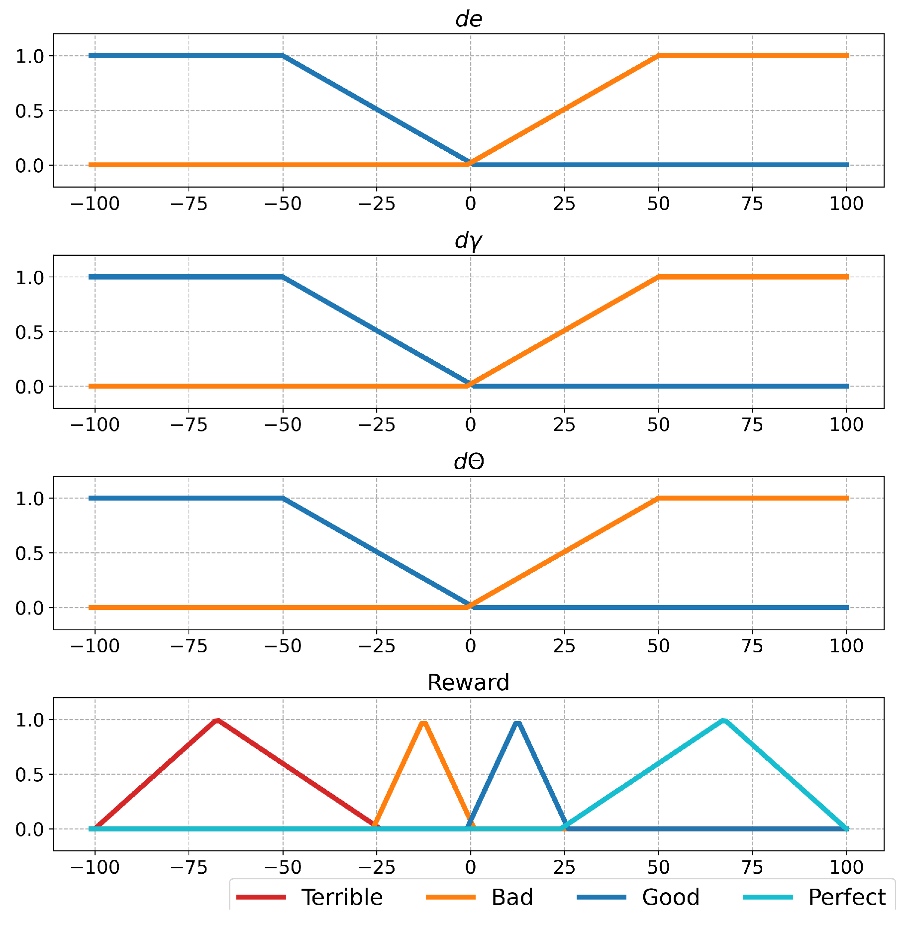
The output of this process is provided to the fuzzy logic function, which evaluates the robot’s proximity to the target, nearby obstacles, and whether its orientation has been corrected. The F u z z y L o g i c ( ) function was designed by using the Mamdani method. Input membership functions are defined for the outputs of the switch functions, and output membership functions are designed symmetrically, as shown in Figure 3. A key consideration in the output functions is creating a balanced scale (e.g., good–bad or perfect–terrible). If negative values (bad–terrible) are prioritized, the robot will focus more on avoiding obstacles than reaching the target. Conversely, if positive values (good–perfect) are prioritized, reaching the target becomes more important than avoiding obstacles. In the first case, the robot may remain stationary, while in the second, it may repeatedly collide with obstacles while heading toward the target. This method consists of the fuzzification of inputs, rule evaluation, aggregation, and defuzzification. Hence, the inputs and output membership functions were given in Figure 3. After this step, the rules were determined, as shown in Table 2. The rule table was created with a focus on the robot’s approach to the target, its movement away from obstacles, and the correction of its orientation.
The aggregation process was carried out after membership functions and the rule table were determined. The result of the aggregation process was evaluated by defuzzification steps and the F u z z y L o g i c ( ) function was formed.

2.2. Agent Structure

The agent making decisions based on rewards is another block of RL. A MLP structure is shown in Figure 4 was used as an agent in the current study.
The MLP structure includes input, hidden, and output cells. The size of input cells equals the size of S ( k ) vector. In the structure, four hidden layers were used and each of hidden layer cells was determined as 2048. Also, rectified linear units (ReLU) were utilized as activation function. These hyper-parameters were chosen according to previous studies [58,59]. Outputs of MLP structure were A ( k ) = [ Δ V x ( k ) ,   Δ W z ( k ) ] . Δ V x ( k ) and Δ W z ( k ) were symbolized as the change in linear and angular velocities. Also, Δ V x ( k ) and Δ W z ( k ) were limited to the range of −0.05 and 0.05. V x ( k ) and W z ( k ) were obtained by using these outputs and Equations (13) and (14).
V x ( k ) = V x ( k 1 ) + Δ V x ( k )
W z ( k ) = W z ( k 1 ) + Δ W z ( k )
After the linear and angular velocities of a robot were obtained, the angular velocity of left ( w l ) and right ( w r ) wheels was calculated by using the kinematic equations given in Equation (15).
V x W z = D 2 D 2 D L D L w l w r
D and L indicate the wheel diameter and wheelbase of a differential-drive mobile robot. D and L parameters of TurtleBot3 Burger robots, that were used in this study, are D T u r t l e B o t = 0.066 m and L T u r t l e B o t = 0.160 m.
RL could be separated into two sub-fields, namely value (Q) and policy ( π ) learning. Policy could be described as π : S P ( A ) function. The main purpose of this function is to generate Markov decision process between state-space ( S ) and action-space ( A ). This process is formed by using current-state ( s t ), action ( a t ), and reward ( r t ) values. These values are used in Equation (16) which shows the discounted reward ( R t ) equation.   
R t = i = t T ς i t r s i ,   a i ,   ς 0 ,   1
where ς represents discount factor. The main purpose of policy-learning RL is that maximizes initial expected distribution J = E [ R 1 ] . Bellman equation is often used in RL as seen in Equation (17).
Q π ( s t ,   a t ) = E r t + ς E Q π s t + 1 ,   a t + 1
Target policy can be described as μ : S A and Q μ ( s t ,   a t ) was given in Equation (18).
Q μ ( s t ,   a t ) = E r t + ς E Q μ s t + 1 ,   μ s t + 1
Loss function depends on Q-learning [60] and can be defined as in Equation (19).
L ( θ Q ) = E Q s t ,   a t θ Q y t 2
y t = r t + ς Q s t + 1 ,   μ s t + 1 θ Q
Function parameters represent θ Q in Equations (19) and (20). PPO, that is, policy-learning methods, were used in this study.

Proximal Policy Optimization Algorithm (PPO)

The PPO algorithm is formed by improving trust-region policy optimization and only first-order optimization is used in this improvement process. The optimization process is realized by utilizing the surrogate function ( L ). L is given in Equation (21).
L ( θ ) = E ^ t m i n R t θ A ^ T ,   c l i p R t θ ,   1 ϵ ,   1 + ϵ A ^ T
R t ( θ ) = π θ a t s t π θ o l d a t s t
The probability ratio is shown as R t in Equation (22). A ^ 1 , , T denotes the advantage estimates. The PPO algorithm is shown in Algorithm 1 for actor–critic network and detailed information about the algorithm can be found in [61].
Algorithm 1 Proximal Policy Optimization Algorithm.
for episode: 1 → M do
       Initialize B a t c h
       Reset environment and obtain s 1
       for iteration: 1 → T do
             a t = π ( s t θ π ) + N t
            Get r t   s t + 1 according to a t
             B a t c h [ s t ,   a t ,   r t ,   s t + 1 ]
            Compute A ^ 1 ,   ,   A ^ T
       end for
       Compute new weight by optimizing surrogate L
       Update networks
end for
In Algorithm 1, the batch and environment restart. The actor network generates an action output according to the state and the noise parameter is added to the action output. This action output is applied to the environment then the next state and reward are calculated. State, action, next state, and reward are stored batch. The advantage A ^ 1 , , T is calculated according to reward and prediction values. The proposed reward function based on fuzzy logic was calculated in response to the action taken by the agent in Algorithm 1 and included in the process as a reward function.Then networks are optimized according to L , which is given in Equation (21).

3. Results and Discussion

In the current study, the first-proposed MLP architecture was trained by using classic and fuzzy logic reward functions using different environments. The determined neural networks were trained during 10 3 episodes and the training process performance of the algorithms can be seen in Table 3. In this table, the α 1 , α 2 , and α 3 were given in Equation (9). C x , A x , and S x ( A x C x ) were shown to be the robot colliding with an obstacle/wall, the robot arriving at the target during training processes, and the score of this sequence, respectively. A l l , L 100 , and B e s t represent the entire training process, the last 100 episodes of the training process, and the best 100 episodes of the training process, respectively. In Table 3, α 1 = 8 , α 2 = 20 , and α 3 = 15 values were found by the trial-and-error method. We tested whether there were better values than these values by increasing or decreasing these values by 25%. These results of the increasing or decreasing process are given in Table 3. The R P r o p o s e d ( k ) function based on fuzzy logic generated a better score than the classic reward function. Also, Table 3 presents the mean ( X ¯ ) and standard deviation ( S D ) calculated over 100-step windows for the last 900 steps, respectively.
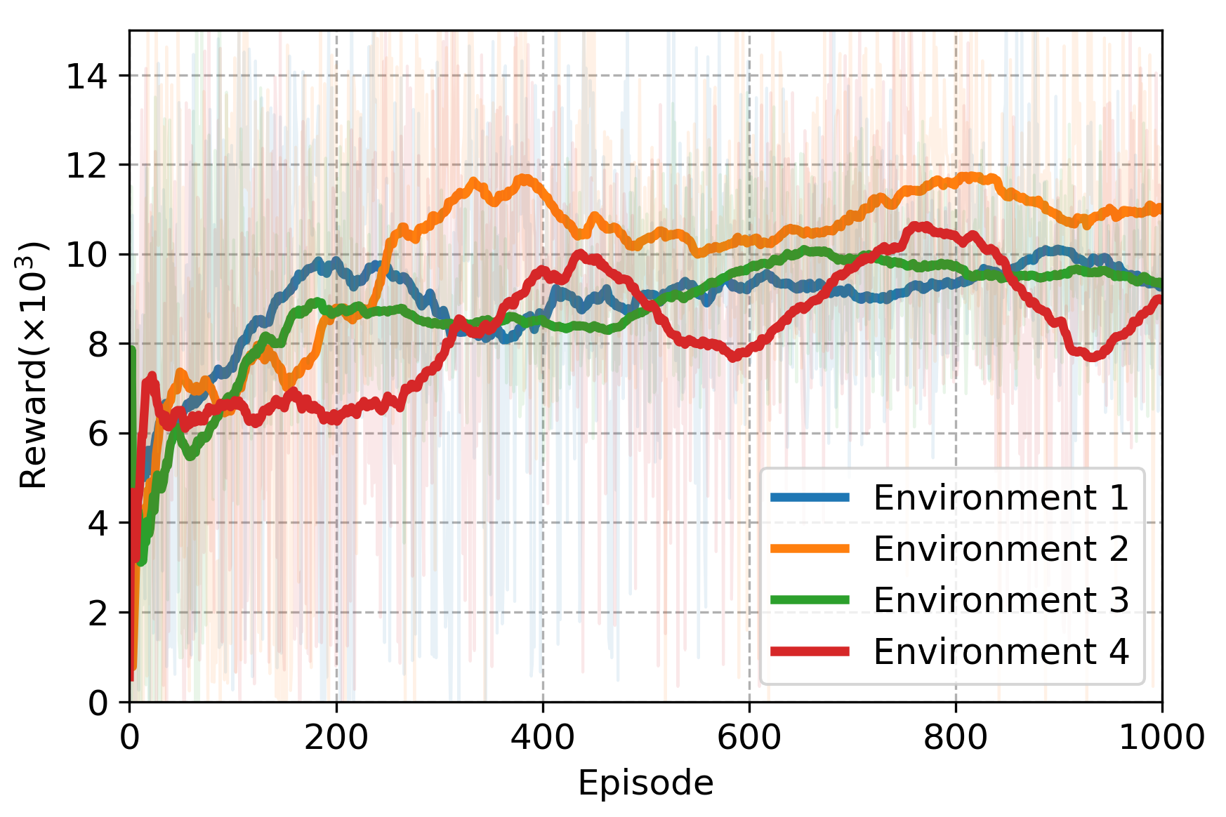
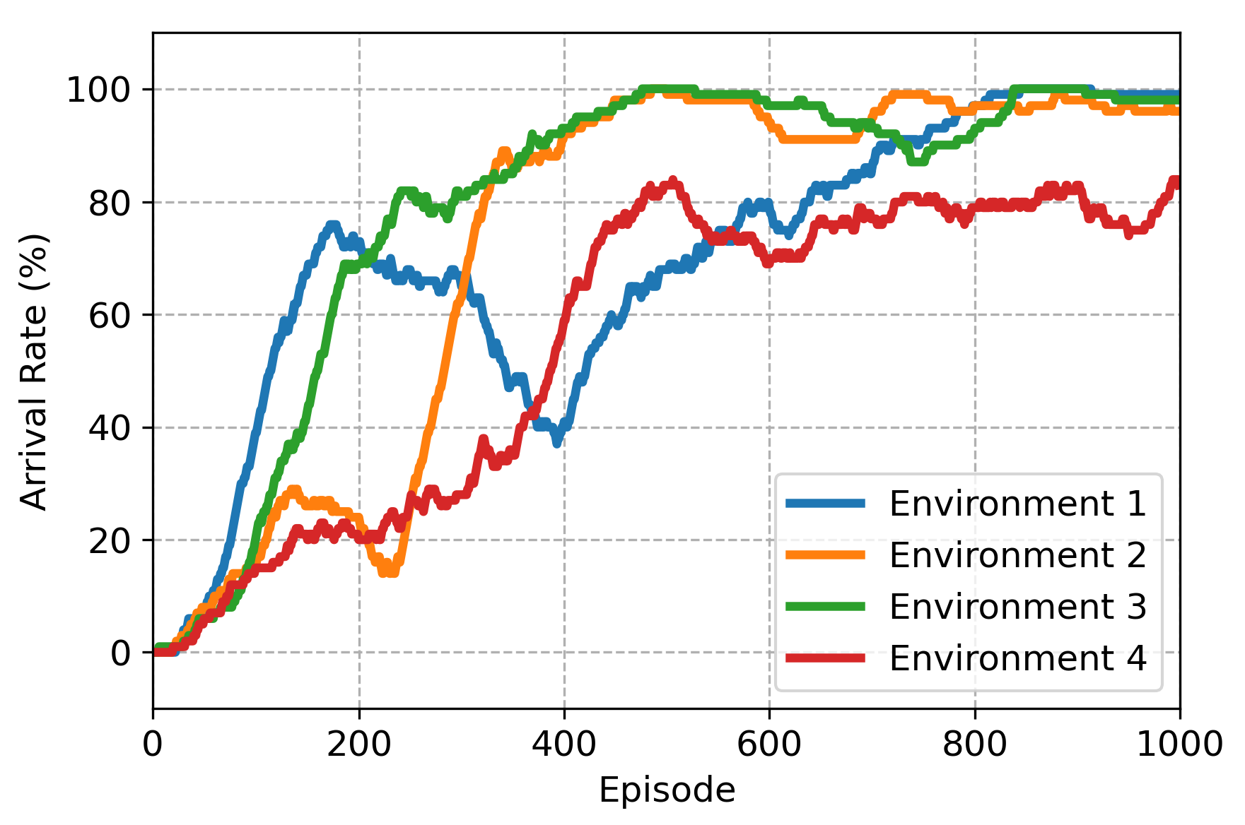
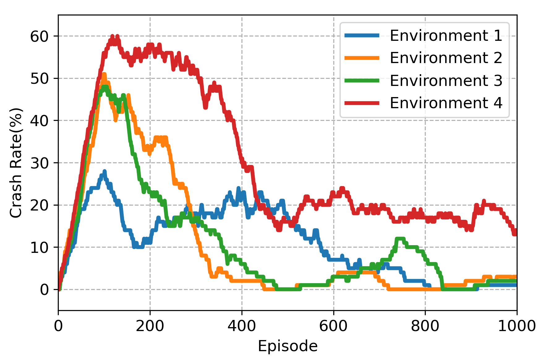
When the proposed fuzzy logic-based reward function was ignored in Table 3, it was seen that there were three highest scoring coefficients for Environment 1. For Environments 2 and 4, the best scores were achieved using coefficients 8, 20, and 15. In Environment 3, the highest score was obtained with coefficients 6, 20, and 15. However, across all four environments, the fuzzy logic-based reward function outperformed the coefficient-based reward functions in generating the best scores. Fuzzy logic-based reward functions have the ability to produce more precise and fine-tuned decisions than classical reward functions. This ability comes from the fact that the reward function, especially the objective function used in reinforcement learning, is more focused on achieving the global maximum value of the reward function. That is, the fuzzy logic approach occurs when the reward function more precisely eliminates not only the global optimum, but also the local optimum. With classical reward functions, the risk of reinforcement learning algorithms getting stuck in local minima is quite high. This can prevent the system from reaching the global optimum and lead to less efficient solutions. However, since fuzzy logic-based methods design the decision-making process to be more flexible and tolerant of uncertainties, such problems are less common. As seen in Table 3, the problem identified using fuzzy logic overcomes the local minimization problem faced by classical approaches. Thus, more precise and optimal decision outputs are obtained. The training performance of the fuzzy logic-based agent is illustrated in Figure 5, Figure 6, Figure 7 and Figure 8. Figure 5 presents the average episode reward, calculated based on the reward values from the last 100 episodes. The robot’s success rate in reaching the target and its collision rate with obstacles or walls is depicted in Figure 6 and Figure 7, respectively, both derived from the last 100 episodes. Finally, Figure 8 displays the training score, determined by subtracting the collision rate from the success rate.
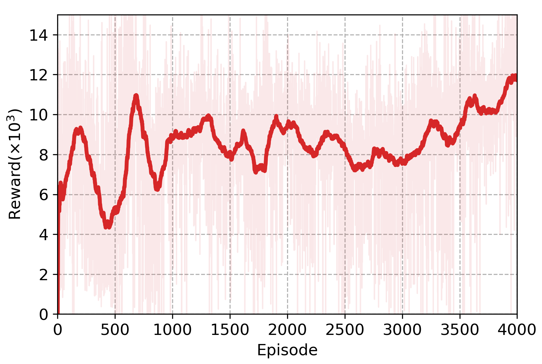
After completing the training process, agents trained with the fuzzy logic-based reward function were tested over 100 steps. The test results were shown in Table 4, where ‘env’ represents the environment. As seen in Table 4, the robot achieved a 100% target-reaching rate in Environments 1–3, while in Environment 4, this rate dropped to 91%. Additionally, the robot collided with an obstacle or wall 7 times during testing in Environment 4. However, when the training period was extended to 4000 steps to address this issue, the robot’s target-reaching rate improved to 100%. The measured reward values during the training of artificial neural network architecture for 4000 episodes were presented in Figure 9. The arrival time was measured from the moment the robot started moving until it successfully reached the target. Additionally, the total distance traveled was recorded as the path taken from the starting position to the target.
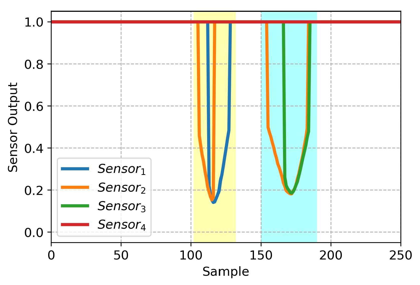
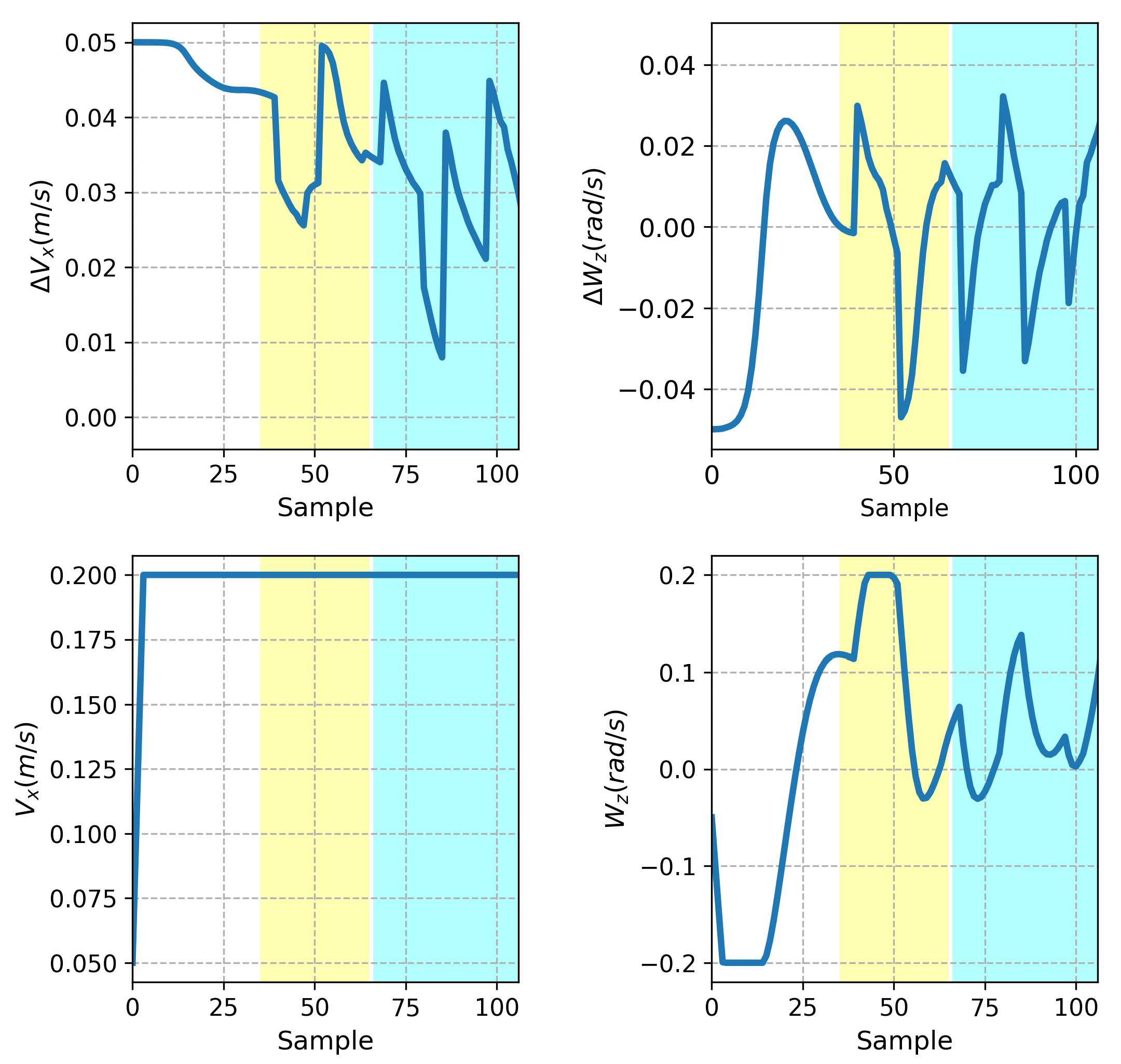
Agents trained in different environments were tested over 100 episodes. Then, in order to examine the proposed method more clearly, it was tested as presented in Figure 10. Parts a and d of Figure 10 present the starting and ending moments of the experiment. Parts b and c depict the moments when the robot encounters the first and second dynamic obstacles, respectively. The signals produced by the sensor model when the robot encounters the first dynamic obstacle were represented by the yellow-colored area in Figure 11. Similarly, when the robot encounters the second dynamic obstacle, the signals generated by the sensor model were represented by the cyan-colored area in Figure 11. The output data of the trained agent corresponding to these colored areas were presented in the Δ V x and Δ W z graphs in Figure 12. The linear ( V x ) and angular velocity ( W z ) of the robot were obtained by aggregating the Δ V x and Δ W z values, as in Figure 12. When Figure 10, Figure 11 and Figure 12 were examined together, the robot escaped by changing its angular velocity when it encountered the first obstacle (which can be seen in the yellow-colored areas in Figure 10b, Figure 11 and Figure 12). When it encountered the second obstacle, it decreased its linear speed to negative and moved in the opposite direction. This is indicated by the linear velocity decreasing from 0.2 m/s to −0.2 m/s. During this movement, it also reduces angular velocity from 0.2 rad/s to approximately 0 rad/s. This is because it wants to avoid the obstacle directly, without using its angular velocity. It reached the target after passing the obstacle (which can be seen in the cyan-colored areas of Figure 10c, Figure 11 and Figure 12).
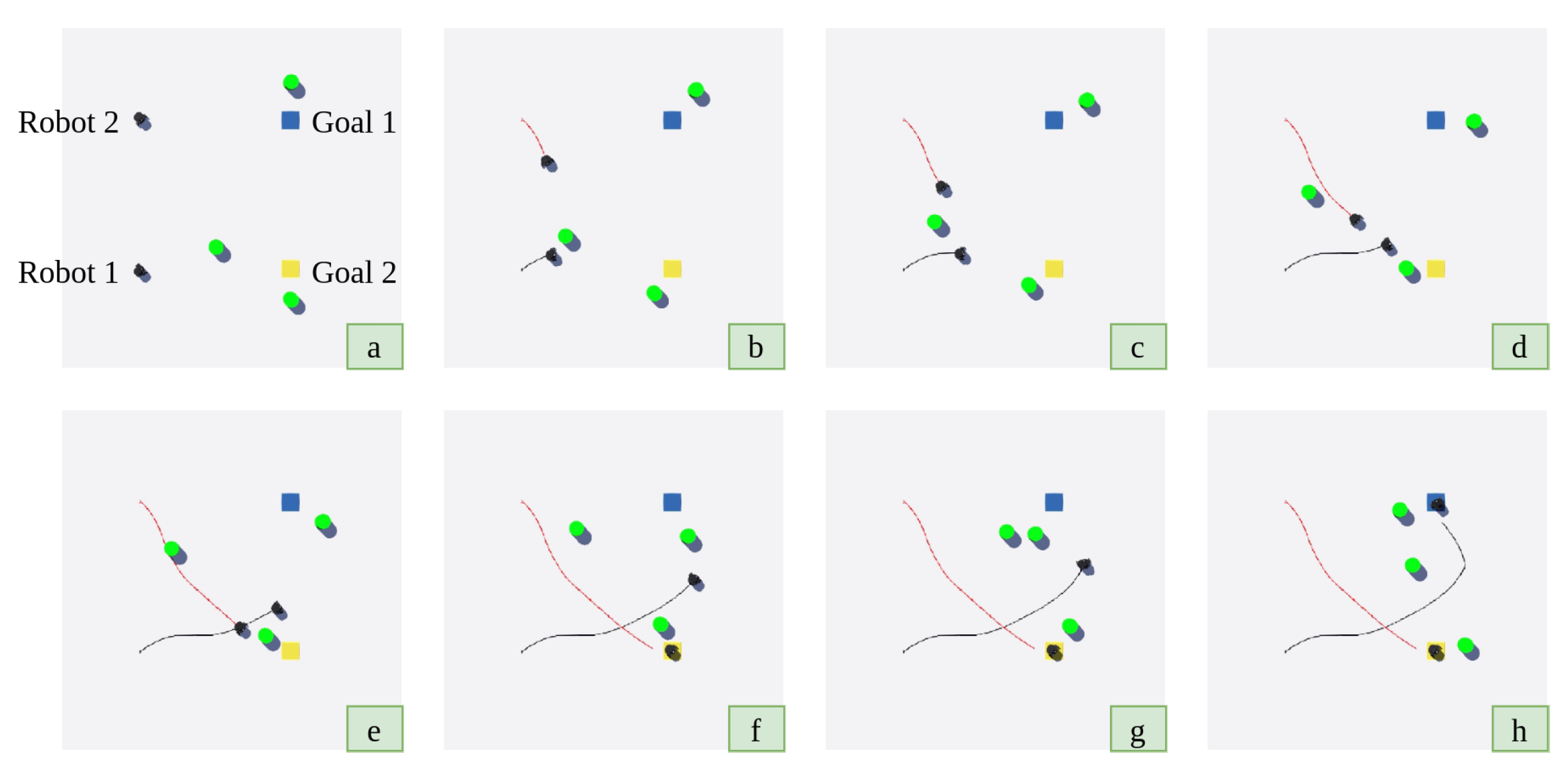
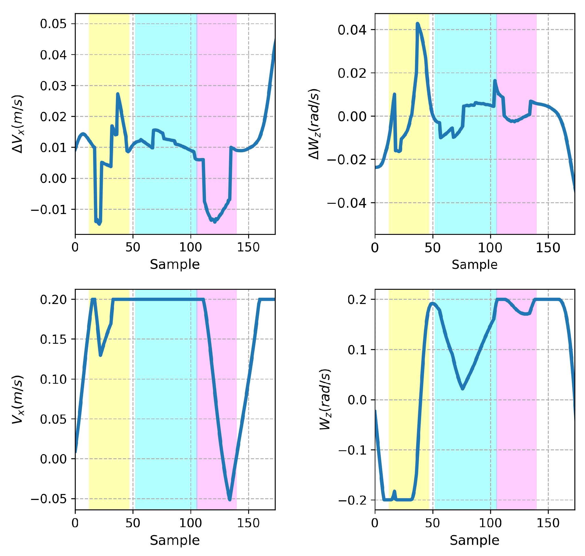
After the training and general testing processes were completed, two robots, with agents trained for Environment 4, were tested in the same environment as presented in Figure 13. Parts a and h of Figure 13 present the starting and ending moments of the experiment. During this test, the paths followed by robot 1 and robot 2 are shown with black and red lines, respectively. As seen in Figure 14, robot 1 detects dynamic obstacles at moments b, d, and f of Figure 13, respectively. These moments were shown in Figure 14 with yellow-, cyan-, and magenta-colored areas. The outputs produced ( Δ V x and Δ W z ) by the agent in response to these fields and the calculated robot velocities ( V x and W z ) are presented in Figure 15. It was observed that robot 1 avoided the first two dynamic obstacles by changing its angular velocity, while it avoided the third obstacle by changing both its angular and linear velocity.
When moments c, d, and e of Figure 13 were examined, robot 2 detected the dynamic obstacle and robot 1, respectively, as can be seen in Figure 16. These moments were shown in Figure 16 with yellow- and cyan-colored areas. The outputs produced ( Δ V x and Δ W z ) by the agent for these environmental effects and the velocity information ( V x and W z ) of robot 2 were visualized in Figure 17. The reaching the target moment of robot 2 was illustrated in Figure 13g. It was observed that robot 2 avoids both the dynamic obstacle and robot 1 by changing the angular velocity.
The advantages of this study are that it proposes a fuzzy logic-based reward function that is more effective than the classical reward function and reduces the size of the artificial neural network architecture by reducing the sensor size. However, the current work has some limitations, such as the dependence on the robot’s position and orientation, the ability to generate responses up to a specific speed of dynamic obstacles, and the wheels can only move up to a maximum speed of 0.2 m/s or rad/s. In general, when Figure 10, Figure 11, Figure 12, Figure 13, Figure 14, Figure 15, Figure 16 and Figure 17 are examined, it is observed that when robots encounter an obstacle, they reduce their maximum linear speed from 0.2 m/s to a stop (approximately 0 m/s) or even decrease it to −0.2 m/s in an attempt to evade the obstacle. This speed adjustment applies not only to linear speed but also to angular speed. During the obstacle-avoidance process, the angular speed, initially at 0.2 rad/s, gradually decreases to around 0 rad/s, assisting in the escape maneuver. The primary factor triggering this avoidance behavior is the absence of a sensor input of 1, meaning the detection of an obstacle.
In this study, a total of four different environments were used, progressing from simple to complex. The first environment contains only one static obstacle, while the second and third environments each include one static and one dynamic obstacle. The fourth and most complex environment consists of one static and two dynamic obstacles. The training process was conducted with a clipping ratio of 0.2 and a discount factor of 0.99, as in the original study [61]. Additionally, the learning rate was set to 10 4 . The training process was carried out using these parameters in all environments. For similar studies, these training parameters are likely to lead to a viable solution. Additionally, the artificial neural network trained in the fourth environment was used for the multi-robot system presented in this study. The successful results obtained have demonstrated the generalization of the training process.
This study has certain limitations. The first limitation is the dependency of the proposed system on the LiDAR sensor. The robot detects obstacles in its environment using the LiDAR sensor. For robots without a LiDAR sensor, alternative distance-measurement sensors capable of perceiving the entire environment can be used. Another limitation is that the study is designed for differential-drive mobile robots. If the developed algorithm is to be applied to Ackerman mobile robots, an appropriate kinematic transformation must be performed.

4. Conclusions

The current study aimed to present a new approach depending on fuzzy logic reward function in order to improve the classical reward function of the RL. For this purpose, an agent that is a major part of RL has formed actor–critical MLP structures. MLP structures were trained to utilize PPO algorithms. The environment, another important part of RL, was designed using the Webots robot simulator program. A state vector containing the robot, obstacle, and goal parameters was determined. The sensor output data were shrunk to reduce the processing load and the neural network size while creating these parameters. Afterwards, two different reward functions were designed as classic and fuzzy logic. The classic reward function was formed by adding or subtracting conventional system parameters. In order to determine the importance of these parameters relative to each other, some coefficients were required when adding or subtracting. In this study, these coefficients were determined by trial-and-error techniques. It was investigated whether there was a better result in their environment by increasing and decreasing established coefficients, as could be seen in Table 3. Then, the fuzzy logic reward function ( R P r o p o s e d ( k ) ) was designed in order to eliminate the problem of searching for the most suitable coefficients. The designed R P r o p o s e d ( k ) function generated the best score in all environments according to Table 3. Then, the fuzzy logic-based trained agents were run through 100 tests in each environment. According to the test results, it was observed that the agents trained in the first three environments had a target arrival rate of 100% in their own environment. For the agent trained in Environment 4, the target arrival rate was measured to be 91% and the rate of hitting an obstacle or wall was 7%. When the training time of the agent was extended up to 4000 episodes, the goal-reaching rate was found to be 100%. Following the general tests, the agent was tested individually and its responses were observed. In individual tests, it was found to effectively avoid dynamic obstacles. The same agent was also tested in another environment with multiple robots. It was observed that the robots in this environment reached the specified targets without hitting any obstacle or robot. According to these results, the shrunk sensor output data performed the requested operation and an effective fuzzy logic-based reward function was successfully created. In future studies, the robust response capability of the system will be improved by applying these methods to reinforcement learning-based systems involving multi-robot systems.

Funding

This research received no external funding.

Institutional Review Board Statement

Not applicable.

Informed Consent Statement

Not applicable.

Data Availability Statement

Data are contained within the article.

Conflicts of Interest

The author declares no conflicts of interest.

References

  1. Ma, Y.; Wang, H.; Xie, Y.; Guo, M. Path planning for multiple mobile robots under double-warehouse. Inf. Sci. 2014, 278, 357–379. [Google Scholar] [CrossRef]
  2. Kumar, N.V.; Kumar, C.S. Development of collision free path planning algorithm for warehouse mobile robot. Procedia Comput. Sci. 2018, 133, 456–463. [Google Scholar] [CrossRef]
  3. Alves, J.G.; Lizarralde, F.; Monteiro, J.C. Control Allocation for Wheeled Mobile Robots Subject to Input Saturation. IFAC—PapersOnLine 2020, 53, 3904–3909. [Google Scholar] [CrossRef]
  4. Qi, C.; Zhu, Y.; Song, C.; Cao, J.; Xiao, F.; Zhang, X.; Xu, Z.; Song, S. Self-supervised reinforcement learning-based energy management for a hybrid electric vehicle. J. Power Sources 2021, 514, 230584. [Google Scholar] [CrossRef]
  5. Jiang, P.; Song, S.; Huang, G. Attention-based meta-reinforcement learning for tracking control of AUV with time-varying dynamics. IEEE Trans. Neural Netw. Learn. Syst. 2021, 33, 6388–6401. [Google Scholar] [CrossRef]
  6. Song, R.; Jang, S.; Wang, Y.; Hanssens, D.M.; Suh, J. Reinforcement learning and risk preference in equity linked notes markets. J. Empir. Financ. 2021, 64, 224–246. [Google Scholar] [CrossRef]
  7. Wang, H.; Jing, J.; Wang, Q.; He, H.; Qi, X.; Lou, R. ETQ-learning: An improved Q-learning algorithm for path planning. Intell. Serv. Robot. 2024, 17, 1–15. [Google Scholar] [CrossRef]
  8. Zhou, Y.; Wang, D.; Liu, L. Exploring unknown environments: Motivated developmental learning for autonomous navigation of mobile robots. Intell. Serv. Robot. 2024, 17, 197–219. [Google Scholar] [CrossRef]
  9. Ganjeh-Alamdari, M.; Alikhani, R.; Perfilieva, I. Fuzzy logic approach in salt and pepper noise. Comput. Electr. Eng. 2022, 102, 108264. [Google Scholar] [CrossRef]
  10. Senthilkumar, G.; Mayavan, T.; Manikandan, H. Prediction of mechanical characteristics of friction welded dissimilar EN 10028P 355 GH steel and AISI 430 steel joint by fuzzy logic analysis. Mater. Today Proc. 2022, 68, 2182–2188. [Google Scholar] [CrossRef]
  11. Mishra, D.K.; Thomas, A.; Kuruvilla, J.; Kalyanasundaram, P.; Prasad, K.R.; Haldorai, A. Design of mobile robot navigation controller using neuro-fuzzy logic system. Comput. Electr. Eng. 2022, 101, 108044. [Google Scholar] [CrossRef]
  12. Boztas, G.; Aydogmus, O. Implementation of Pure Pursuit Algorithm for Nonholonomic Mobile Robot using Robot Operating System. Balk. J. Electr. Comput. Eng. 2021, 9, 337–341. [Google Scholar] [CrossRef]
  13. Xu, L.; Cao, M.; Song, B. A New Approach to Smooth Path Planning of Mobile Robot Based on Quartic Bezier Transition Curve and Improved PSO Algorithm. Neurocomputing 2021, 473, 98–106. [Google Scholar] [CrossRef]
  14. Hou, W.; Xiong, Z.; Wang, C.; Chen, H. Enhanced ant colony algorithm with communication mechanism for mobile robot path planning. Robot. Auton. Syst. 2021, 148, 103949. [Google Scholar] [CrossRef]
  15. Miao, C.; Chen, G.; Yan, C.; Wu, Y. Path planning optimization of indoor mobile robot based on adaptive ant colony algorithm. Comput. Ind. Eng. 2021, 156, 107230. [Google Scholar] [CrossRef]
  16. Deng, X.; Li, R.; Zhao, L.; Wang, K.; Gui, X. Multi-obstacle path planning and optimization for mobile robot. Expert Syst. Appl. 2021, 183, 115445. [Google Scholar] [CrossRef]
  17. Tripathy, H.K.; Mishra, S.; Thakkar, H.K.; Rai, D. CARE: A Collision-Aware Mobile Robot Navigation in Grid Environment using Improved Breadth First Search. Comput. Electr. Eng. 2021, 94, 107327. [Google Scholar] [CrossRef]
  18. Mylvaganam, T.; Sassano, M. Autonomous collision avoidance for wheeled mobile robots using a differential game approach. Eur. J. Control. 2018, 40, 53–61. [Google Scholar] [CrossRef]
  19. Li, H.; Savkin, A.V. An algorithm for safe navigation of mobile robots by a sensor network in dynamic cluttered industrial environments. Robot. Comput.-Integr. Manuf. 2018, 54, 65–82. [Google Scholar] [CrossRef]
  20. Maldonado-Ramirez, A.; Rios-Cabrera, R.; Lopez-Juarez, I. A visual path-following learning approach for industrial robots using DRL. Robot. Comput.-Integr. Manuf. 2021, 71, 102130. [Google Scholar] [CrossRef]
  21. Schmitz, A.; Berthet-Rayne, P. Using Deep-Learning Proximal Policy Optimization to Solve the Inverse Kinematics of Endoscopic Instruments. IEEE Trans. Med. Robot. Bionics 2020, 3, 273–276. [Google Scholar] [CrossRef]
  22. Wen, S.; Wen, Z.; Zhang, D.; Zhang, H.; Wang, T. A multi-robot path-planning algorithm for autonomous navigation using meta-reinforcement learning based on transfer learning. Appl. Soft Comput. 2021, 110, 107605. [Google Scholar] [CrossRef]
  23. Tan, X.; Chng, C.B.; Su, Y.; Lim, K.B.; Chui, C.K. Robot-assisted training in laparoscopy using deep reinforcement learning. IEEE Robot. Autom. Lett. 2019, 4, 485–492. [Google Scholar] [CrossRef]
  24. Tallamraju, R.; Saini, N.; Bonetto, E.; Pabst, M.; Liu, Y.T.; Black, M.J.; Ahmad, A. Aircaprl: Autonomous aerial human motion capture using deep reinforcement learning. IEEE Robot. Autom. Lett. 2020, 5, 6678–6685. [Google Scholar] [CrossRef]
  25. Gangapurwala, S.; Mitchell, A.; Havoutis, I. Guided constrained policy optimization for dynamic quadrupedal robot locomotion. IEEE Robot. Autom. Lett. 2020, 5, 3642–3649. [Google Scholar] [CrossRef]
  26. Zhang, D.; Bailey, C.P. Obstacle avoidance and navigation utilizing reinforcement learning with reward shaping. In Artificial Intelligence and Machine Learning for Multi-Domain Operations Applications II; SPIE: Bellingham, WA, USA, 2020; Volume 11413, pp. 500–506. [Google Scholar]
  27. Zhao, T.; Wang, M.; Zhao, Q.; Zheng, X.; Gao, H. A path-planning method based on improved soft actor-critic algorithm for mobile robots. Biomimetics 2023, 8, 481. [Google Scholar] [CrossRef]
  28. Wong, M.F.; Tan, C.W. Aligning Crowd-Sourced Human Feedback for Reinforcement Learning on Code Generation by Large Language Models. arXiv 2025, arXiv:2503.15129. [Google Scholar] [CrossRef]
  29. Zheng, R.; Dou, S.; Gao, S.; Hua, Y.; Shen, W.; Wang, B.; Liu, Y.; Jin, S.; Liu, Q.; Zhou, Y.; et al. Secrets of rlhf in large language models part i: Ppo. arXiv 2023, arXiv:2307.04964. [Google Scholar]
  30. Azlan, N.; Zainudin, F.; Yusuf, H.; Toha, S.; Yusoff, S.; Osman, N. Fuzzy logic controlled miniature LEGO robot for undergraduate training system. In Proceedings of the 2007 2nd IEEE Conference on Industrial Electronics and Applications, Harbin, China, 23–25 May 2007; pp. 2184–2188. [Google Scholar]
  31. Singh, N.H.; Thongam, K. Mobile robot navigation using fuzzy logic in static environments. Procedia Comput. Sci. 2018, 125, 11–17. [Google Scholar] [CrossRef]
  32. Pandey, A.; Parhi, D.R. MATLAB simulation for mobile robot navigation with hurdles in cluttered environment using minimum rule based fuzzy logic controller. Procedia Technol. 2014, 14, 28–34. [Google Scholar] [CrossRef]
  33. Xu, J.X.; Guo, Z.Q.; Lee, T.H. Design and implementation of a Takagi–Sugeno-type fuzzy logic controller on a two-wheeled mobile robot. IEEE Trans. Ind. Electron. 2012, 60, 5717–5728. [Google Scholar] [CrossRef]
  34. Nguyen, A.T.; Vu, C.T. Mobile Robot Motion Control Using a Combination of Fuzzy Logic Method and Kinematic Model. In Intelligent Systems and Networks; Springer: Singapore, 2022; pp. 495–503. [Google Scholar]
  35. Karaduman, B.; Tezel, B.T.; Challenger, M. Enhancing BDI agents using fuzzy logic for CPS and IoT interoperability using the JaCa platform. Symmetry 2022, 14, 1447. [Google Scholar] [CrossRef]
  36. Lu, J.; Ma, G.; Zhang, G. Fuzzy Machine Learning: A Comprehensive Framework and Systematic Review. IEEE Trans. Fuzzy Syst. 2024, 32, 3861–3878. [Google Scholar] [CrossRef]
  37. Xie, Z.; Sun, T.; Kwan, T.; Wu, X. Motion control of a space manipulator using fuzzy sliding mode control with reinforcement learning. Acta Astronaut. 2020, 176, 156–172. [Google Scholar] [CrossRef]
  38. Khater, A.A.; El-Nagar, A.M.; El-Bardini, M.; El-Rabaie, N.M. Online learning of an interval type-2 TSK fuzzy logic controller for nonlinear systems. J. Frankl. Inst. 2019, 356, 9254–9285. [Google Scholar] [CrossRef]
  39. Zhang, C.; Zou, W.; Cheng, N.; Gao, J. Trajectory tracking control for rotary steerable systems using interval type-2 fuzzy logic and reinforcement learning. J. Frankl. Inst. 2018, 355, 803–826. [Google Scholar] [CrossRef]
  40. Vemireddy, S.; Rout, R.R. Fuzzy reinforcement learning for energy efficient task offloading in vehicular fog computing. Comput. Netw. 2021, 199, 108463. [Google Scholar] [CrossRef]
  41. Chen, L.; Hu, X.; Tang, B.; Cheng, Y. Conditional DQN-based motion planning with fuzzy logic for autonomous driving. IEEE Trans. Intell. Transp. Syst. 2020, 23, 2966–2977. [Google Scholar] [CrossRef]
  42. Hinojosa, W.M.; Nefti, S.; Kaymak, U. Systems control with generalized probabilistic fuzzy-reinforcement learning. IEEE Trans. Fuzzy Syst. 2010, 19, 51–64. [Google Scholar] [CrossRef]
  43. Chen, G.; Lu, Y.; Yang, X.; Hu, H. Reinforcement learning control for the swimming motions of a beaver-like, single-legged robot based on biological inspiration. Robot. Auton. Syst. 2022, 154, 104116. [Google Scholar] [CrossRef]
  44. Liu, J.; Lu, H.; Luo, Y.; Yang, S. Spiking neural network-based multi-task autonomous learning for mobile robots. Eng. Appl. Artif. Intell. 2021, 104, 104362. [Google Scholar] [CrossRef]
  45. Xiao, H.; Chen, C.; Zhang, G.; Chen, C.P. Reinforcement learning-driven dynamic obstacle avoidance for mobile robot trajectory tracking. Knowl.-Based Syst. 2024, 297, 111974. [Google Scholar] [CrossRef]
  46. Cui, T.; Yang, X.; Jia, F.; Jin, J.; Ye, Y.; Bai, R. Mobile robot sequential decision making using a deep reinforcement learning hyper-heuristic approach. Expert Syst. Appl. 2024, 257, 124959. [Google Scholar] [CrossRef]
  47. Yan, C.; Chen, G.; Li, Y.; Sun, F.; Wu, Y. Immune deep reinforcement learning-based path planning for mobile robot in unknown environment. Appl. Soft Comput. 2023, 145, 110601. [Google Scholar] [CrossRef]
  48. Sun, H.; Zhang, C.; Hu, C.; Zhang, J. Event-triggered reconfigurable reinforcement learning motion-planning approach for mobile robot in unknown dynamic environments. Eng. Appl. Artif. Intell. 2023, 123, 106197. [Google Scholar] [CrossRef]
  49. Bai, Z.; Pang, H.; He, Z.; Zhao, B.; Wang, T. Path Planning of Autonomous Mobile Robot in Comprehensive Unknown Environment Using Deep Reinforcement Learning. IEEE Internet Things J. 2024, 11, 22153–22166. [Google Scholar] [CrossRef]
  50. Choi, J.; Lee, G.; Lee, C. Reinforcement learning-based dynamic obstacle avoidance and integration of path planning. Intell. Serv. Robot. 2021, 14, 663–677. [Google Scholar] [CrossRef]
  51. Khnissi, K.; Jabeur, C.B.; Seddik, H. A smart mobile robot commands predictor using recursive neural network. Robot. Auton. Syst. 2020, 131, 103593. [Google Scholar] [CrossRef]
  52. Duguleana, M.; Mogan, G. Neural networks based reinforcement learning for mobile robots obstacle avoidance. Expert Syst. Appl. 2016, 62, 104–115. [Google Scholar] [CrossRef]
  53. Shantia, A.; Timmers, R.; Chong, Y.; Kuiper, C.; Bidoia, F.; Schomaker, L.; Wiering, M. Two-stage visual navigation by deep neural networks and multi-goal reinforcement learning. Robot. Auton. Syst. 2021, 138, 103731. [Google Scholar] [CrossRef]
  54. Low, E.S.; Ong, P.; Cheah, K.C. Solving the optimal path planning of a mobile robot using improved Q-learning. Robot. Auton. Syst. 2019, 115, 143–161. [Google Scholar] [CrossRef]
  55. Lin, G.; Zhu, L.; Li, J.; Zou, X.; Tang, Y. Collision-free path planning for a guava-harvesting robot based on recurrent deep reinforcement learning. Comput. Electron. Agric. 2021, 188, 106350. [Google Scholar] [CrossRef]
  56. Mabu, S.; Tjahjadi, A.; Hirasawa, K. Adaptability analysis of genetic network programming with reinforcement learning in dynamically changing environments. Expert Syst. Appl. 2012, 39, 12349–12357. [Google Scholar] [CrossRef]
  57. Li, S.; Ding, L.; Gao, H.; Chen, C.; Liu, Z.; Deng, Z. Adaptive neural network tracking control-based reinforcement learning for wheeled mobile robots with skidding and slipping. Neurocomputing 2018, 283, 20–30. [Google Scholar] [CrossRef]
  58. Bingol, M.C. Reinforcement Learning-Based Safe Path Planning for a 3R Planar Robot. Sakarya Univ. J. Sci. 2022, 26, 127–134. [Google Scholar] [CrossRef]
  59. Bingol, M.C. Development of Neural Network Based on Deep Reinforcement Learning to Compensate for Damaged Actuator of a Planar Robot. In Proceedings of the Global Conference on Engineering Research (Globcer’21), Bandırma, Türkiye, 2–5 June 2021. [Google Scholar]
  60. Watkins, C.J.; Dayan, P. Q-learning. Mach. Learn. 1992, 8, 279–292. [Google Scholar] [CrossRef]
  61. Schulman, J.; Wolski, F.; Dhariwal, P.; Radford, A.; Klimov, O. Proximal policy optimization algorithms. arXiv 2017, arXiv:1707.06347. [Google Scholar]
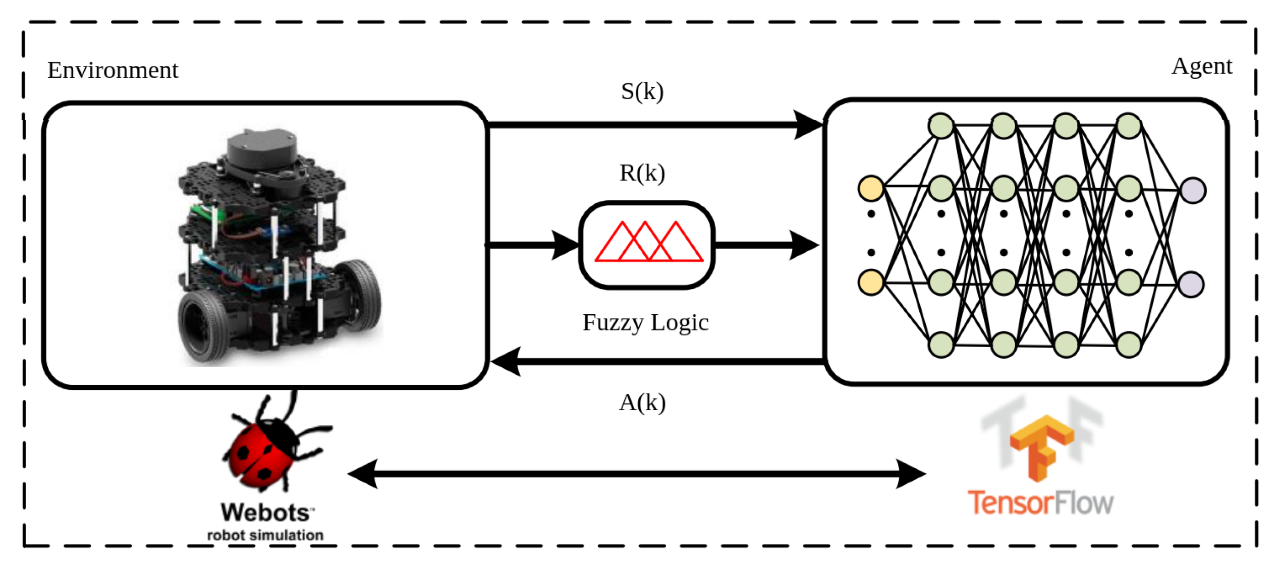
Figure 1. Block diagram of proposed system.
Electronics 14 01593 g001
Figure 2. Designed environments.
Electronics 14 01593 g002
Figure 3. Fuzzy logic membership functions.
Electronics 14 01593 g003
Figure 4. The used MLP structure.
Electronics 14 01593 g004
Figure 5. Episodic and average reward values throughout agent training using the R P r o p o s e d ( k ) reward function.
Electronics 14 01593 g005
Figure 6. The rate of arrival at the goal of robot throughout agent training using the R P r o p o s e d ( k ) reward function.
Electronics 14 01593 g006
Figure 7. The rate of the robot crashing into an obstacle or wall throughout agent training using the R P r o p o s e d ( k ) reward function.
Electronics 14 01593 g007
Figure 8. The score calculated throughout agent training using the R P r o p o s e d ( k ) reward function.
Electronics 14 01593 g008
Figure 9. Episodic and average reward values throughout agent training using R P r o p o s e d ( k ) reward function over 4000 episodes.
Electronics 14 01593 g009
Figure 10. A test of the trained agent using the R P r o p o s e d ( k ) reward function in Environment 4.
Electronics 14 01593 g010
Figure 11. Sensor signals generated during the test were shown in Figure 10.
Electronics 14 01593 g011
Figure 12. The generated output and calculated robot velocities according to the sensor signals shown in Figure 11.
Electronics 14 01593 g012
Figure 13. A test of two robots by the trained agent using the R P r o p o s e d ( k ) reward function.
Electronics 14 01593 g013
Figure 14. The sensor signals of robot 1 generated during the test are shown in Figure 13.
Electronics 14 01593 g014
Figure 15. The generated output and calculated robot 1 velocities according to the sensor signals shown in Figure 14.
Electronics 14 01593 g015
Figure 16. The sensor signals of robot 2 generated during the test were shown in Figure 13.
Electronics 14 01593 g016
Figure 17. The generated output and calculated robot 2 velocities according to the sensor signals shown in Figure 16.
Electronics 14 01593 g017
Table 1. Webots robot simulator parameters.
ParameterValue
Gravity9.81
Time Step128
Constraint Force Mixing10−5
Error-Reduction Parameter0.2
Optimal Thread Count1
Physics Disable Time1
Physics Disable Linear Threshold0.01
Physics Disable Angular Threshold0.01
Line Scale0.1
Drag Force Scale30
Drag Torque Scale5
Table 2. Rule table of fuzzy logic-based reward function.
Rules de d γ d θ Reward
1ifGoodGoodGoodthenPerfect
2ifGoodGoodBadthenGood
3ifGoodBadGoodthenGood
4ifGoodBadBadthenBad
5ifBadGoodGoodthenGood
6ifBadGoodBadthenBad
7ifBadBadGoodthenBad
8ifBadBadBadthenTerrible
Table 3. Comparisons of the training results of classical and fuzzy logic-based reward functions.
α 1 α 2 α 3 C ALL C( X ¯  ± SD) A ALL A( X ¯  ± SD) S ALL S( X ¯  ± SD) C L 100 A L 100 S L 100 C Best A Best S Best
Environment 16201524924.0 ± 9.5461463.5 ± 17.7036539.4 ± 26.2513736079386
10201525324.1 ± 18.2867270.3 ± 19.1941946.3 ± 37.3517755829492
8151524425.0 ± 15.5759160.3 ± 17.4534735.34 ± 31.082888629492
8251532732.2 ± 17.4240640.6 ± 35.71798.4 ± 51.8710817178881
8201218317.5 ± 6.2568270.4 ± 15.2949952.9 ± 20.3310897979285
8201819819.0 ± 16.6371774.3 ± 25.2851955.2 ± 41.6011897829492
8201521419.6 ± 11.0065868.7 ± 19.3744449.1 ± 29.5514806659287
R P r o p o s e d ( k ) 11010.4 ± 7.8774876.0 ± 17.9263865.6 ± 25.57199980100100
Environment 26201546646.5 ± 10.8037838.9 ± 13.07−88−7.6 ± 23.37374811296132
10201544043.7 ± 12.7538439.3 ± 22.75−56−4.5 ± 34.72335825187961
8151546247.8 ± 15.4241140.7 ± 21.49−51−7.0 ± 35.92168064168064
8251550050.4 ± 5.1035436.3 ± 12.80−146−14.1 ± 14.8144539445410
8201239538.1 ± 15.9846748.4 ± 21.927210.3 ± 37.65305424207858
8201847849.3 ± 13.4543043.6 ± 18.30−48−5.7 ± 30.81306737247551
8201527825.4 ± 14.9360464.1 ± 21.9232638.6 ± 36.74306232108777
R P r o p o s e d ( k ) 1099.27 ± 14.3177379.6 ± 28.5764470.4 ± 42.67396930100100
Environment 36201524322.7 ± 15.4266769.3 ± 19.5042446.5 ± 34.8413826949187
10201522220.3 ± 13.3065167.6 ± 19.7942947.3 ± 32.7410837398980
8151544545.5 ± 14.2539939.6 ± 18.03−46−5.9 ± 31.35167761167862
8251573776.4 ± 34.4324621.9 ± 3266−491−54.4 ± 67.088877988880
8201228827.9 ± 9.7158460.6 ± 17.1829632.7 ± 26.30246440118776
8201843542.8 ± 7.5848851.0 ± 12.27538.2 ± 19.63435411257348
8201527327.0 ± 13.8358159.2 ± 20.7830832.1 ± 34.4310867698879
R P r o p o s e d ( k ) 1129.7 ± 11.7484987.6 ± 17.2473777.9 ± 28.93298960100100
Environment 46201552252.1 ± 15.9338639.6 ± 21.10−136−12.5 ± 36.50385921296738
10201549449.6 ± 12.7741942.6 ± 13.58−75−6.9 ± 26.02425412316332
8151557657.8 ± 11.2934835.8 ± 11.92−228−22.0 ± 22.684946−3366327
8251544443.7 ± 13.9748449.6 ± 17.50405.9 ± 30.90385921227351
8201248147.4 ± 16.2743244.8 ± 16.67−49−2.5 ± 32.77425614256944
8201851451.4 ± 16.6840740.9 ± 17.35−107−10.5 ± 33.81336633217049
8201547045.8 ± 18.9944447.2 ± 22.77−261.4 ± 41.505140−11157964
R P r o p o s e d ( k ) 29929.7 ± 16.1359860.5 ± 24.0629930.8 ± 40.18148369158469
Table 4. The testing of an agent trained using the R P r o p o s e d ( k ) reward function during 100 episodes.
Arrival Time (s)Distance Traveled (m)
EnvCrashedArrivedScoreMinMaxMedianMinMaxMedian
1010010015.87240.3223.8083.1228.024.705
2010010018.94434.17624.0643.7166.7744.747
3010010016.0034.0422.1443.1337.7484.362
47918417.15232.0024.0643.2036.2524.637
Disclaimer/Publisher’s Note: The statements, opinions and data contained in all publications are solely those of the individual author(s) and contributor(s) and not of MDPI and/or the editor(s). MDPI and/or the editor(s) disclaim responsibility for any injury to people or property resulting from any ideas, methods, instructions or products referred to in the content.