Enhanced GAIN-Based Missing Data Imputation for a Wind Energy Farm SCADA System

Abstract

The integrity and reliability of wind turbine electrical data (such as active power, voltage, current, etc.) are crucial for operational monitoring, fault diagnosis, and predictive analysis in wind energy systems. However, due to various reasons such as hardware failures, network communication issues, environmental interference, and human errors, data gaps still exist in the Supervisory Control and Data Acquisition (SCADA) systems. Existing multivariate wind power time series imputation methods face two main limitations: (1) inadequate handling of continuous missing patterns (band missing and feature missing) and (2) insufficient utilization of spatiotemporal and feature correlations among wind turbines. To address these shortcomings, this study proposes an imputation framework that includes two types of SCADA data missing scenarios in wind turbines. For band missing, the framework leverages similar wind turbine data matching to explore spatiotemporal correlations in wind power data. For feature missing, the framework focuses on feature correlations in wind power data using Pearson coefficients and normalized mutual information. Additionally, we designed a novel Dual-Type Deep Convolutional Generative Adversarial Imputation Network (DT-DCGAIN) model within this framework to impute different types of missing data. Finally, by evaluating the proposed method on real-world wind farm SCADA datasets, it achieved a 13.91% to 28.32% improvement in Root Mean Square Error (RMSE). Ablation experiments on the model further validated the contributions of each correlation extraction module.

1. Introduction

Wind turbines are typically equipped with various types of sensors to monitor the operational status of the units in real time and record operational data. During turbine operation, these sensors generate a large amount of real-time data, with sampling frequencies ranging from per second, per minute, to per hour, among other time scales [1]. These data are not only transmitted to the SCADA controller of the wind turbine for real-time monitoring and anomaly detection tasks [2,3] but are also stored in the SCADA system to support subsequent power system dispatching [4,5], stability analysis [6,7], and wind power generation forecasting [8,9]. However, extensive research on wind farm operation and maintenance indicates that data gaps in SCADA systems for wind turbines are inevitable due to factors such as sensor malfunctions, communication interruptions, system maintenance, and human operational errors [10]. Data-driven wind turbines have stringent requirements for data integrity and quality in the aforementioned downstream tasks [11]. Therefore, effectively addressing SCADA system data gaps and accurately imputing missing data for wind turbines hold significant research importance and practical application value.

Current methods for missing data imputation can be broadly categorized into three types: statistical-based methods, classical machine-learning-based methods, and deep-learning-based methods. The first category relies primarily on traditional mathematical formulas and probabilistic distribution models. These methods often assume linear relationships between variables (e.g., linear interpolation) or simple probability distributions (e.g., Gaussian distribution), making it difficult to effectively capture the complex nonlinear dynamics inherent in wind turbine data [11]. Additionally, since wind power data are inherently multivariate time series, statistical-based methods struggle to exploit spatiotemporal correlations and feature interdependencies among variables, often resulting in significant biases in imputation results. In contrast, classical machine-learning-based methods improve imputation accuracy by learning similarities and relationships between features. However, these methods require step-by-step learning over the entire dataset, and given the typically large scale of SCADA system datasets in wind farms, computational efficiency becomes a major limitation. Furthermore, as the missing data rate increases, the performance of these methods significantly declines, restricting their effectiveness in practical applications.

In recent years, significant progress has been made in the application of artificial intelligence technologies to wind energy power systems, with many researchers proposing deep-learning-based methods for missing data imputation. For example, Cao et al. further introduced the Bidirectional Recurrent Imputation for Time Series (BRITS) model [12], which leverages the hidden states of Bidirectional Recurrent Neural Networks (BRNN) [13] to simultaneously capture forward and backward dependencies in wind turbine time series data, thereby improving the accuracy of missing value estimation. Additionally, Du et al. developed a time series imputation model based on a self-attention mechanism (SAITS) [14], enabling efficient learning of time series features and imputation of missing values. Although these methods excel in modeling global characteristics of time series, the inherent complexity, time-varying nature, and randomness of wind power data make it challenging for existing models to fully capture its essential features. Furthermore, these deep learning methods belong to the category of discriminative models, which are primarily used for tasks such as classification and regression and cannot generate new data that resemble the distribution of the original data. This limitation restricts their potential in tasks like data augmentation and diverse data analysis. In contrast, generative models can generate missing parts or enhanced samples by modeling the probability distribution of the data, demonstrating significant advantages in handling missing data and out-of-distribution samples. Generative adversarial models, due to their powerful ability to model complex distributions, as well as their diversity and reliability in data imputation, have gradually become mainstream in the field of missing data imputation. Goodfellow et al. first proposed the Generative Adversarial Network (GAN) [15], which can generate high-quality data samples through the adversarial training mechanism of the generator and discriminator. However, this model primarily targets imputation tasks for non-time-series data and has limited effectiveness in handling time series data missing problems. To address this issue, Yoon et al. improved GAN and proposed the Generative Adversarial Imputation Network (GAIN) [16], providing a new solution for imputing missing time series data. To tackle the potential mode collapse problem during the training of the GAIN model, Neves et al. introduced the WSGAIN-CP model [17], which enhances model stability by replacing the original JS divergence with the Wasserstein distance. Guo et al. focused on the imputation of multivariate time series data and proposed the Multivariate Time Series Generative Adversarial Network (MTS-GAN) [18]. Building on this, Lai et al. designed a multi-task learning mechanism based on autoencoders (AEMTLDY) [19], effectively addressing the challenges of multi-dimensional data imputation. Additionally, Zhao et al. proposed an improved Complete Ensemble Empirical Mode Decomposition with Adaptive Noise (ICEEMDAN) method and applied GAIN to the preprocessing of wind power data, constructing the ICEEMDAN-GAIN model [20], which successfully achieved the imputation of missing wind power data. However, existing research has not systematically considered the spatiotemporal correlations in multivariate time series data from wind farm SCADA systems or the feature correlations among wind turbines, leading to significant deviations between the imputation results and actual conditions. Moreover, most studies assume that SCADA system data is missing at random (MAR), and when these methods are applied to continuous missing or non-random missing scenarios, the accuracy of the generated data often fails to meet practical requirements. Additionally, the original GAIN model may face issues such as vanishing gradients or mode collapse during training, which limits the model’s generalization ability and imputation effectiveness.

To address the issues identified in the current research landscape, this study proposes a data imputation framework tailored for missing data scenarios in wind farm SCADA systems. This framework covers two typical data missing scenarios: (1) the case where all feature data of a single wind turbine is missing over a continuous time period, and (2) the case where a specific feature data of all wind turbines is missing over a continuous time period. The framework is based on an improved generative adversarial network model, namely, the Dual-Type Deep Convolutional Generative Adversarial Imputation Network (DT-DCGAIN), aiming to achieve high-precision imputation for different missing types. The DT-DCGAIN model introduces several enhancements over the original GAIN model: First, it incorporates the Kantorovich–Rubenstein dual form of the Wasserstein distance to measure the discrepancy between generated data and real data, effectively mitigating mode collapse and vanishing gradient issues. Second, it employs Deep Convolutional Neural Networks (DCNNs) as the core architecture for both the generator and discriminator, significantly improving the model’s ability to learn complex data features and enhancing the stability of the training process. Additionally, the model includes a similar wind turbine data matching module to exploit spatiotemporal correlations in wind power data and a feature selection module to extract feature correlations, further improving imputation accuracy. The primary goal of this study is to design an efficient data imputation framework for wind turbines and significantly enhance the accuracy of missing data imputation through the improved GAIN method. The effectiveness of the proposed method is validated through experiments on real SCADA datasets. The main contributions of this paper are as follows:

This paper innovatively proposes a unified data imputation framework that integrates two typical data missing types in wind turbines (band missing and feature missing). By designing a similar wind turbine data matching module and a feature selection module, the framework enhances the imputation accuracy of the model under different data missing scenarios.

To address issues such as mode collapse, vanishing gradients, and insufficient feature extraction capabilities in the GAIN model, this paper introduces the Kantorovich–Rubenstein dual form of the Wasserstein distance in the discriminator and employs Deep Convolutional Neural Networks (DCNNs) as the core architecture for both the generator and discriminator. These improvements effectively enhance the model’s training stability, feature learning capability, and diversity in generating missing data.

To validate the effectiveness of the proposed method, extensive comparative experiments were conducted on real SCADA datasets, comparing the performance with various mainstream data imputation benchmark methods. Additionally, ablation experiments were systematically performed to verify the contributions of each improved module to the model’s performance, fully demonstrating the superiority and robustness of the proposed method.

The remaining content of this paper is structured as follows: Section 2 introduces the main types and characteristics of missing time series data in wind farms; Section 3 elaborates on the proposed DT-DCGAIN model and its core methodologies; Section 4 conducts experimental research based on real SCADA datasets and presents and analyzes the experimental results; and Section 5 concludes the paper.

2. Related Work

Types of Time-Series Data Missingness in Wind Farms

In current academia, missing data are generally categorized into three types: Missing Completely at Random (MCAR), Missing at Random (MAR), and Missing Not at Random (MNAR) [21]. However, this classical classification framework primarily targets non-time-series data (e.g., tabular data, image data) and exhibits limitations when applied to wind farm time-series data. Notably, continuous missing—a prevalent phenomenon in wind farm SCADA systems [22]—demonstrates distinctive industry-specific causes, including but not limited to meteorological factors such as gust interference, antenna icing, and lightning strikes that lead to monitoring interruptions. Based on the characteristics of wind farm operational data, this study proposes a novel dichotomous classification system: random missing data and continuous missing data. The continuous missing data can be further subdivided according to its spatiotemporal distribution characteristics: band missing: the absence of all monitoring parameters for a single turbine unit over continuous time periods; feature missing: the absence of a specific monitoring parameter across all turbine units over continuous time periods. As illustrated in Figure 1, this classification system more accurately reflects the actual missing patterns in wind farm time-series data by incorporating industry-specific missing patterns, thereby providing theoretical foundations for subsequent data quality management.

Random missing: Random missing refers to the situation where the missing data of wind turbines occurs randomly, with no apparent correlation to time, features, or other variables. This type of missing data is typically caused by transient communication failures, sensor anomalies, or brief system interruptions. In SCADA systems, random missing is a fundamental type of missing data and is the primary focus of most current research efforts.

Band Missing: Band missing refers to the situation where all feature data of a single wind turbine is continuously missing over a specific time period, often manifesting as data gaps in one or more time intervals. This type of missing data is primarily caused by equipment failures, communication interruptions, or system maintenance operations.

Feature Missing: Feature Missing refers to the concurrent absence of a specific feature dataset (e.g., gearbox temperature, generator speed, etc.) across all wind turbines while other feature data remain intact. This phenomenon typically results from failures in specific sensor components within the measurement system, manifesting as systematic data acquisition anomalies.

3. Materials and Methods

3.1. Overall Structure of the Integrated Data Imputation Framework

This paper proposes an integrated data imputation framework aimed at addressing two typical electrical data missing issues in wind turbine SCADA systems. Figure 2 illustrates the overall structure of the imputation framework and its core components.

The electrical data of wind turbines are influenced by the randomness and variability of wind energy, leading to significant differences across different time periods. When a turbine experiences long-term data missing, relying solely on its historical data for imputation may not be sufficiently accurate. To address this issue, the framework employs the SWDM module to calculate the spatiotemporal correlations between the missing turbine and other complete turbines, thereby assisting in imputing the missing data. When all turbines miss a specific electrical feature over a certain period, directly using band missing data to train the DT-DCGAIN model may limit the imputation effectiveness. Since the electrical features of wind turbines are correlated, the missing feature can be imputed using other strongly correlated and complete features as well as the turbine’s historical data. To achieve this, the framework adopts the SCFS module to screen highly correlated feature data, enabling accurate and reasonable imputation of missing values.

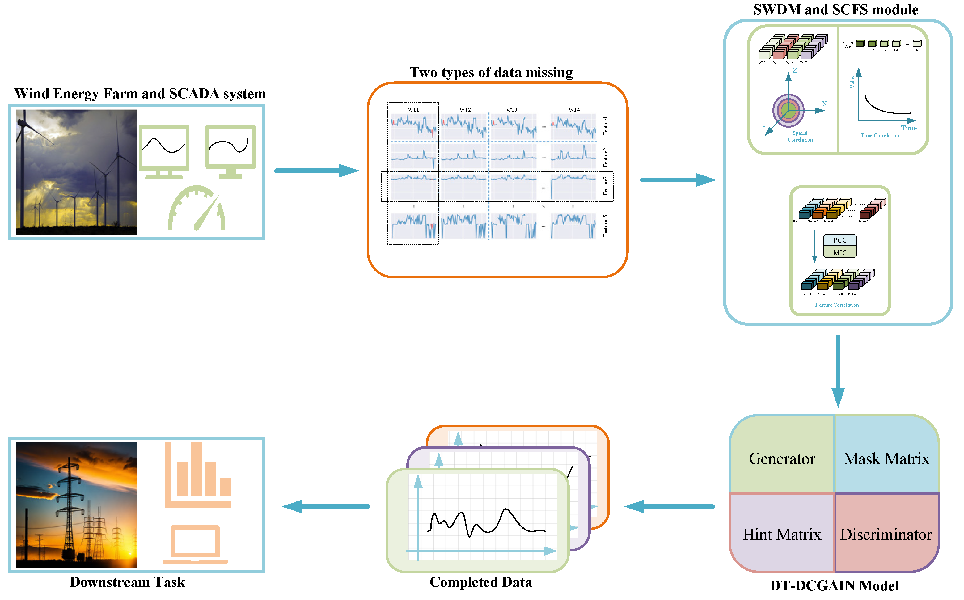
3.2. Similar Wind Turbine Data Matching Module

In terms of natural environment, “similar wind turbines” should meet geographical and climatic conditions including [23] whether they are located in the same wind farm; have similar terrain and topography; have comparable surface roughness; or involve environmental factors like temperature, humidity, and air pressure. This ensures the turbines operate under similar external environments and avoids data bias caused by environmental factors.

Regarding turbine operation, “similar wind turbines” should have identical technical parameters such as turbine model, rated power, rotor diameter, and hub height. Additionally, we emphasize the impact of operational status (e.g., load level, maintenance condition) on data matching to ensure the selected turbines operate under similar working conditions.

Furthermore, the spatiotemporal correlation between different wind turbines is a highly complex concept that is influenced not only by operational conditions among turbines, but also by natural factors such as terrain, topography, wind speed, and regional microclimate [24]. The wind turbines selected in this study are located in flat plain areas with relatively uniform wind speed distribution and minimal regional climatic variations. Therefore, the spatiotemporal correlation primarily considers the operational conditions between different wind turbines. Based on this, the SWDM module (Similar Wind Turbine Data Matching Module) is employed to screen the operational status of wind turbines, ensuring the accuracy and reliability of data matching. The SCADA data from the selected wind farm will be described in the experimental section (Section 4).

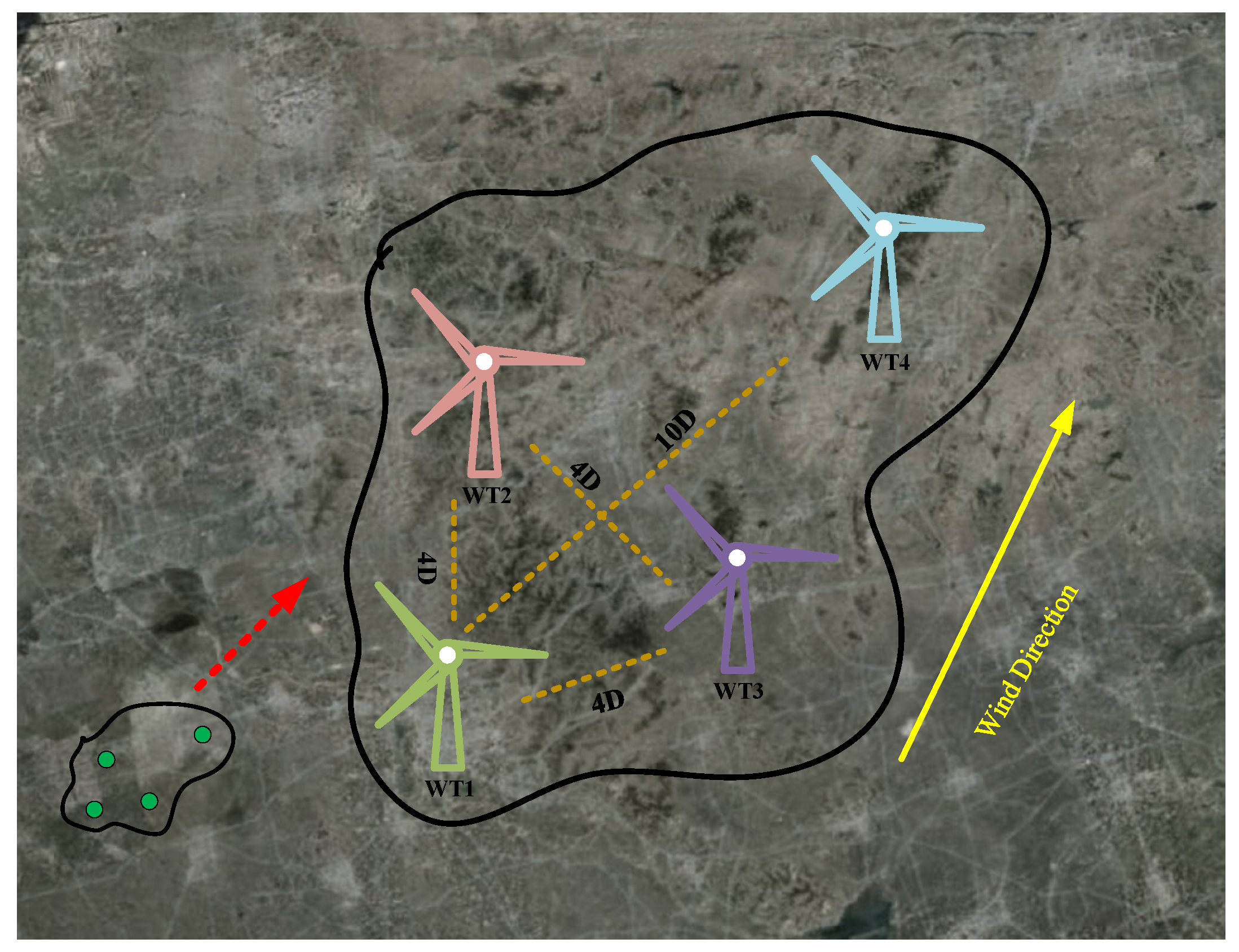
In the task of wind power data imputation, spatiotemporal correlation is a key factor in building efficient models. Temporal correlation helps predict the future variation trends of electrical data in wind turbines, while spatial correlation can extract similar data patterns from neighboring wind turbines, thereby improving the accuracy of data interpolation. Figure 3 illustrates the spatiotemporal correlation of active power data between any two wind turbines in a wind farm.

From a temporal perspective, the feature data of wind turbines at adjacent time points typically exhibit strong similarity and correlation, but this correlation gradually weakens as the time interval increases. This temporal dependency can be quantified using the temporal autocorrelation coefficient [25]. For example, the temporal autocorrelation coefficient for active power can be calculated using the following formula:

$${\rho }_T={\displaystyle \frac{{\displaystyle \sum _{t=t_0}^{T-\Delta t}(P_t-\overline{P})(P_{t+\Delta t}-\overline{P})}}{{\displaystyle \sum _{t=t_0}^T{(P_t-\overline{P})}^2}}}$$

(1)

where ${\rho }_T$ represents the temporal autocorrelation coefficient of the wind turbine’s features; $\Delta t$ represents the time lag; $\overline{P}$ represents the average value of active power; $P_t$ and $P_{t+\Delta t}$ represent the active power data at times $t$ and $t+\Delta t$, respectively; and $t_0$ and $T$ represent the initial and final moments, respectively.

From a spatial perspective, neighboring turbines within a wind farm, due to being in similar geographical environments, exhibit high similarity in their wind power characteristics, reflecting spatial correlation. The strength of this correlation can be quantified using the Spearman rank correlation coefficient. A higher coefficient indicates greater similarity in the feature data of the turbines and stronger spatial correlation.

$${\rho }_S={\displaystyle \frac{{\displaystyle \sum _{i=1}^n(R(F_{X_i})-\overline{R(F_{X_i})})}(R(F_{Y_i})-\overline{R(F_{Y_i})})}{\sqrt{{\displaystyle \sum _{i=1}^n{(R(F_{X_i})-\overline{R(F_{X_i})})}^2{\displaystyle \sum _{i=1}^n{(R(F_{Y_i})-\overline{R(F_{Y_i})})}^2}}}}}$$

(2)

In the formula, ${\rho }_S$ represents the Spearman rank correlation coefficient between two wind turbines; $F_{X_i}$ and $F_{Y_i}$ represent the $i$th feature data (e.g., active power) of wind turbine $X$ and wind turbine $Y$, respectively; $n$ is the number of data samples; and $R$ and $\overline{R}$ represent the ranks and average ranks.

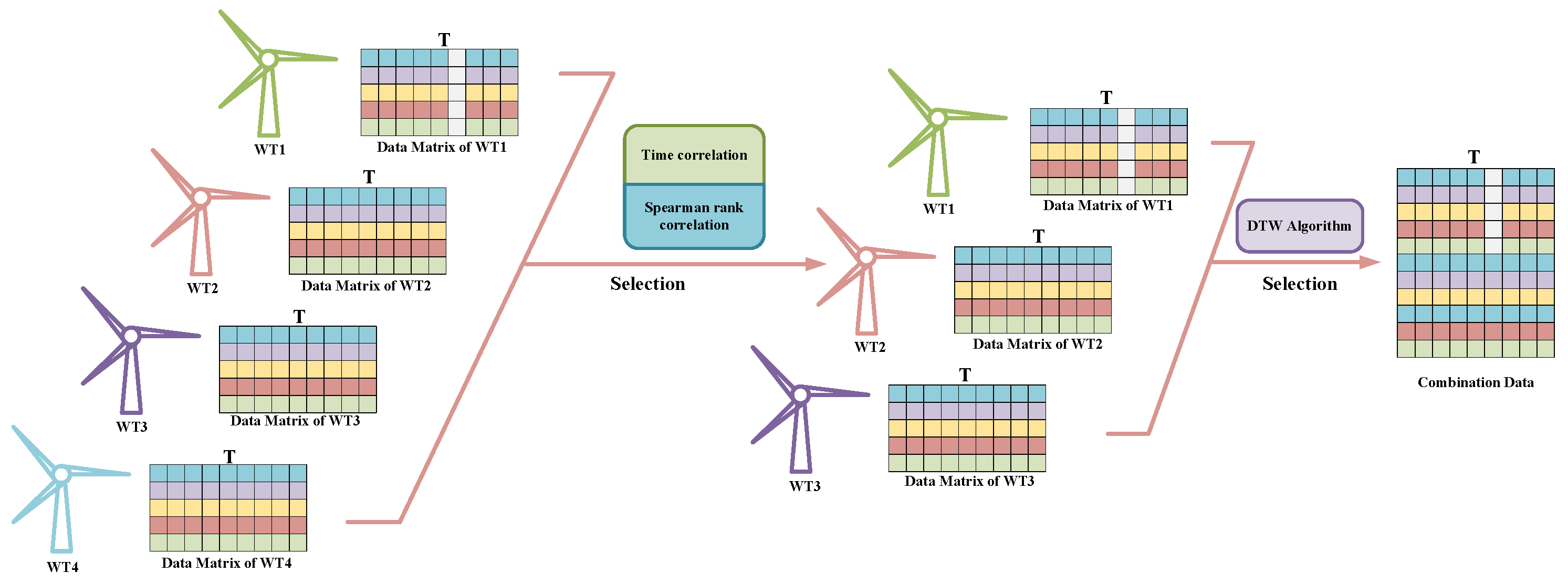
For the convenience of theoretical analysis, this paper defines the turbine with missing data as the target turbine, its electrical data as the target data, and the turbines with high spatiotemporal correlation to the target turbine as reference turbines, with their electrical data defined as reference data. After initially screening the reference turbine data through spatiotemporal correlation, to enhance the reliability of DT-DCGAIN model training, it is necessary to further screen the reference turbine data with higher correlation to the target turbine using the Dynamic Time Warping (DTW) algorithm [26]. The following elaborates on this process in two steps.

Step 1: Construct a cumulative distance matrix $L$.

First, represent the target turbine data and reference turbine data in matrix form:

$$\begin{array}{l}{F}_{ref}={[X_1,X_2,\cdots ,X_w]}^T=\left[\begin{array}{cccc}{x}_{1,1}& x_{1,2}& \dots & x_{1,T_{X_1}}\\ x_{2,1}& x_{2,2}& \cdots & x_{2,T_{X_2}}\\ ⋮& ⋮& & ⋮\\ x_{w,1}& x_{w,1}& \cdots & x_{w,T_{X_k}}\end{array}\right],F_{tgt}={[Y_1,Y_2,\cdots ,Y_w]}^T=\left[\begin{array}{cccc}{y}_{1,1}& { \mathrm{y}}_{1,2}& \dots & y_{1,T_{Y_1}}\\ y_{2,1}& { \mathrm{y}}_{2,2}& \cdots & y_{2,T_{Y_2}}\\ ⋮& ⋮& & ⋮\\ y_{w,1}& { \mathrm{y}}_{w,1}& \cdots & y_{w,T_{Y_k}}\end{array}\right]\end{array}$$

(3)

where the reference wind turbine $F_{ref}$ data matrix and the target wind turbine $F_{tgt}$ data matrix contain all the feature data sequences; $X_i$ and $Y_i$ represent the $i$-th feature of the reference and target wind turbines, respectively; and $T_{X_i}$ and $T_{Y_i}$ represent the time series lengths of the $i$-th feature for the reference and target wind turbines, respectively, and they may not be equal.

Then, construct a cumulative distance matrix $L$ of dimension $T_{X_k}\times T_{Y_k}$, where each element is calculated using the following formula:

$$\left\{\begin{array}{l}{l}_{1,1}=\sqrt{{(x_{i,1}-y_1)}^2}\\ l_{m,1}={\displaystyle {\sum }_{m=2}^{T_{X_i}}\sqrt{{(x_{i,m}-y_1)}^2}+l_{1,1},m\in [2,} T_{X_i}]\\ l_{1,n}={\displaystyle {\sum }_{n=2}^{T_{Y_i}}\sqrt{{(x_{i,1}-y_n)}^2}+l_{1,1}, n\in [2,} T_{Y_i}]\\ l_{m,n}=\sqrt{{(x_{i,m}-y_n)}^2}+\min \{l_{m-1,n},l_{m,n-1},l_{m-1,n-1}\},\\ \hspace{1em}\hspace{1em} \hspace{0.17em}m\in [2,T_{X_i}],n\in [2,T_{Y_i}]\end{array}\right.$$

(4)

where $x$ and $y$ represent the data of $T_{X_i}$ and $T_{Y_i}$, respectively; $l_{m,n}$ denotes the matrix element; and $m$, $n$ indicate the row and column numbers.

After constructing the cumulative distance matrix $L$, the equation can be obtained: $\gamma \left(X_i,Y_i\right)=l_{T_{X_i},T_{Y_i}}$, where $\gamma \left(X_i,Y_i\right)$ is the minimum warping path distance, and $l_{T_{X_i},T_{Y_i}}$ is the last element of $L$.

Step 2: Construct a similarity contribution matrix $C$ of dimension $W\times k$ and set a reasonable threshold. By performing a weighted average on the elements of each row in matrix $C$, a similarity contribution vector $\overrightarrow{C}$ is obtained, where each element represents the similarity score between a specific feature data of the target wind turbine and the corresponding feature data of the reference wind turbine. Subsequently, each element in the vector is compared with a preset threshold, and elements greater than the threshold are selected to form a new reference wind turbine feature dataset $F_{ref}^{\prime }$, which serves as the conditional input data for training the DT-DCGAIN model.

The similarity contribution matrix $C$ can be constructed using the following formula:

$$c_{i,T_{X_j}}={\displaystyle \frac{\max (\gamma \left(X_i,Y_i\right))-\gamma \left(X_i,Y_i\right)}{\max (\gamma \left(X_i,Y_i\right))}}$$

(5)

$$\begin{array}{l}C=\left[\begin{array}{cccc}{c}_{1,T_{X_1}}& c_{1,T_{X_2}}& \dots & c_{1,T_{X_k}}\\ c_{2,T_{X_1}}& c_{2,T_{X_2}}& \cdots & c_{2,T_{X_k}}\\ ⋮& ⋮& & ⋮\\ c_{w,T_{X_1}}& c_{w,T_{X_2}}& \cdots & c_{w,T_{X_k}}\end{array}\right]\end{array}$$

(6)

$$F_{ref}^{\prime }={[{X_1}^{\prime },{X_2}^{\prime },\cdots ,{X_w}^{\prime }]}^T$$

(7)

where $c_{i,T_{X_j}}$ is the original similarity contribution matrix $C$.

Furthermore, each element of the similarity contribution vector $\overrightarrow{C}$ can be calculated as follows:

$$c_j={\displaystyle \frac{{\displaystyle \sum _{i=1}^k{c}_{j,T_{X_i}}}}{k}},j=1,2\dots ,w$$

(8)

$$\overrightarrow{C}=[c_1,c_2,\cdots ,c_w]$$

(9)

where $c_j$ is the element of the similarity contribution vector $\overrightarrow{C}$.

Finally, the data filtered for similarity to each electrical feature data of the target wind turbine is combined to form the reference dataset:

$$\begin{array}{l}{F}_{ref}^{\prime }={[{X_1}^{\prime },{X_2}^{\prime },\cdots ,{X_w}^{\prime }]}^T=\left[\begin{array}{cccc}{x}_{1,1}^{\prime }& x_{1,2}^{\prime }& \dots & x_{1,T_{X_1}}^{\prime }\\ x_{2,1}^{\prime }& x_{2,2}^{\prime }& \cdots & x_{2,T_{X_2}}^{\prime }\\ ⋮& ⋮& & ⋮\\ x_{w,1}^{\prime }& x_{w,2}^{\prime }& \cdots & x_{w,T_{X_k}}^{\prime }\end{array}\right]\end{array}$$

(10)

where $F_{ref}^{\prime }$ is the feature data of the reference wind turbine obtained after the final screening.

Figure 4 illustrates the schematic diagram of the data screening process for the Similar Wind Turbine Data Matching (SWDM) module. Through the processing of this module, data with higher similarity to the target turbine can be screened and used as training inputs for the DT-DCGAIN model.

3.3. Strongly Correlated Feature Selection Module

The feature data of wind turbines are interdependent; for example, changes in wind speed and direction directly affect power output and generator speed, reflecting correlations among features. Therefore, when a specific feature (such as active power) is missing in SCADA data, feature correlation becomes crucial for imputation. Given the large volume of SCADA data, to improve imputation efficiency and accuracy, it is necessary to screen variables highly correlated with the missing feature. This paper employed the Pearson correlation coefficient and the maximal information coefficient methods to select strongly correlated features, optimizing the imputation process.

First, the Pearson Correlation Coefficient (PCC) method is used to perform an initial screening of all feature data of the target turbine:

$$PCC(X,Y)={\displaystyle \frac{E(XY)-E(X)E(Y)}{\sqrt{E(X^2)-E^2(X)}\sqrt{E(Y^2)-E^2(Y)}}}$$

(11)

where $X$ and $Y$ represent two turbine features in the target wind turbine data.

After the initial feature screening using the PCC method, the Maximal Information Coefficient (MIC) method is further applied for secondary feature screening to identify key features that are highly correlated with the missing feature (such as nonlinear, exponential, and periodic features):

$$MIC(x,y)=\underset{{\eta }_x{\eta }_y<B(\eta )}{\max }{\displaystyle \frac{I(x,y)}{{\log }_2(\min \{{\eta }_x,{\eta }_y\})}}$$

(12)

$$\begin{array}{ll}\hfill I(x,y)& =H(x)+H(y)-H(x,y)\hfill \\ \hfill & ={\displaystyle \sum _{i=1}^{{\eta }_x}p(x_i){\log }_2\frac{1}{p(x_i)}+}{\displaystyle \sum _{i=1}^{{\eta }_y}p(y_i){\log }_2\frac{1}{p(y_i)}}\hfill \\ \hfill & \hspace{1em}-{\displaystyle \sum _{i=1}^{{\eta }_x}{\displaystyle \sum _{i=1}^{{\eta }_y}p(x_i{y}_i)}}{\log }_2{\displaystyle \frac{1}{p(x_i{y}_i)}}\end{array}$$

(13)

where ${\eta }_x$ and ${\eta }_y$ represent the number of interval divisions for target wind farm features $X$ and $Y$, $B(\eta )$ represents the total number of interval divisions ($B(\eta )<\sqrt{n}$, $n$ are the total number of samples), $I(x,y)$ represents the mutual information between $X$ and $Y$, $H(x)$ and $H(y)$ represent the entropy of features $X$ and $Y$, and $H(x,y)$ represents their joint entropy.

Figure 5 illustrates the schematic diagram of the data screening process for the Strongly Correlated Feature Selection Module (SCFS). Through the processing of this module, feature variables with higher correlation to the missing feature data of the target turbine can be screened and used as training inputs for the DT-DCGAIN model, thereby enhancing the model’s imputation accuracy and reliability.

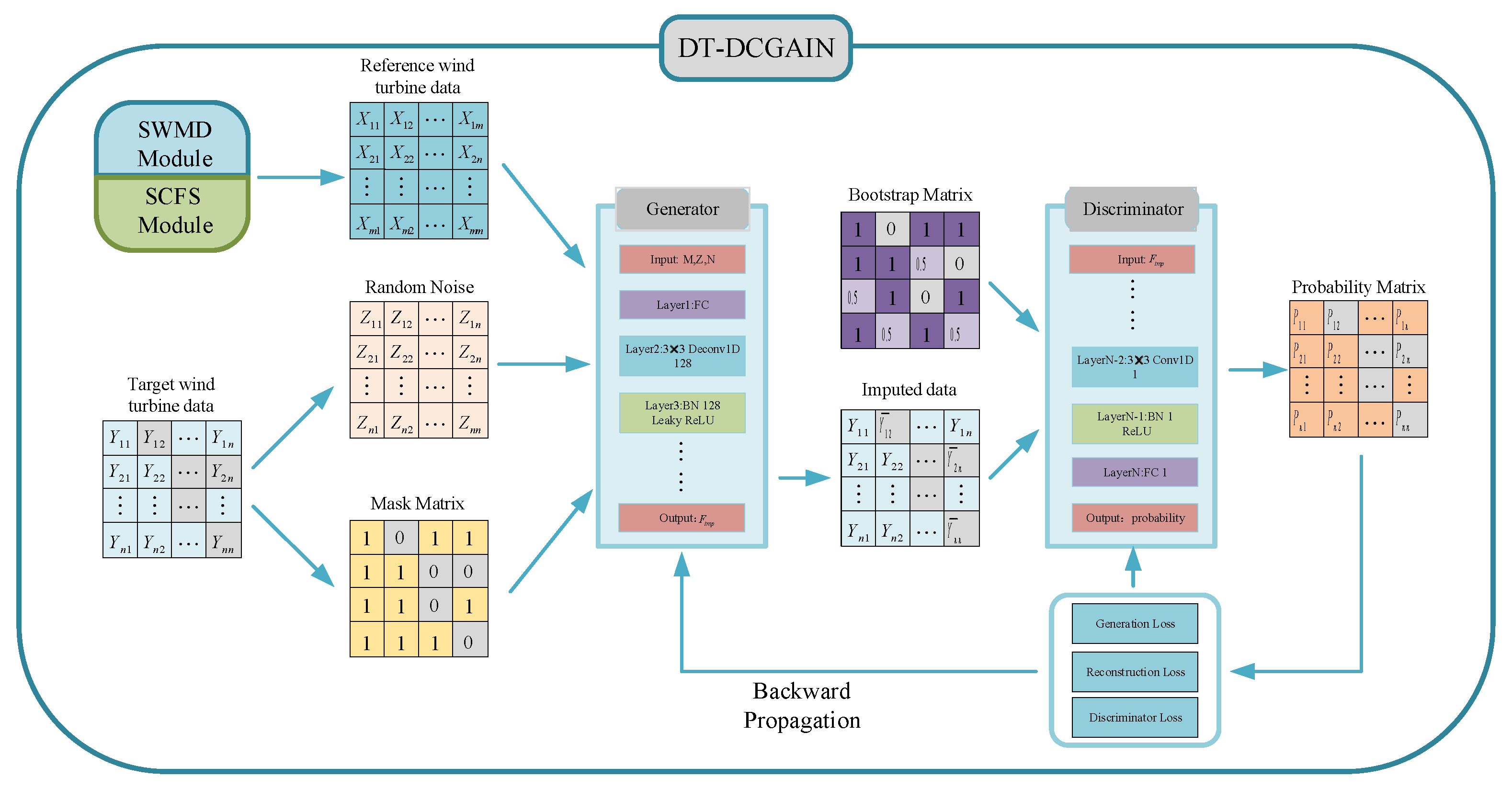
3.4. The DT-DCGAIN Model

The GAIN model is an improved version of the Generative Adversarial Network (GAN), specifically designed for imputing missing values in time series data [16]. By introducing a mask matrix $M$ (mask matrix) to identify missing and observed values in the data, this mechanism significantly enhances the efficiency and accuracy of traditional GANs in missing data imputation tasks. However, as mentioned in the introduction, the GAIN model still has certain limitations when applied to wind farm data imputation tasks. Therefore, this paper proposes the DT-DCGAIN model, whose structure is illustrated in Figure 6.

The model further improves upon the GAIN model, with its core idea derived from the zero-sum game theory in game theory and applies this theory to the adversarial training framework between the generator and the discriminator. The mathematical theoretical foundation of the model will be elaborated in detail below.

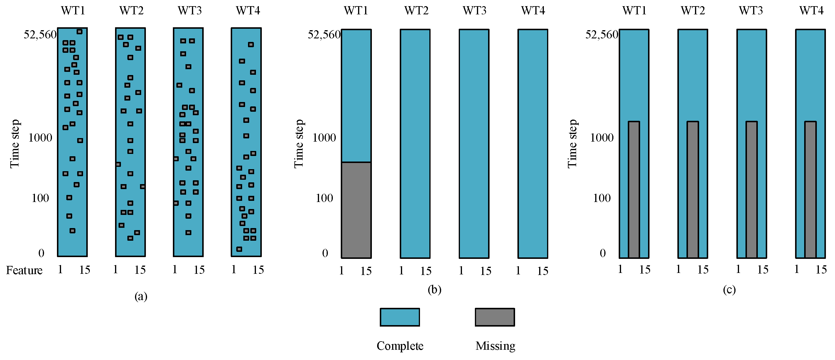
When the wind farm data are missing in a band pattern, the relationship between the real data $F_{tgt}$ of the target wind turbine and the mask matrix $M$ is $F_{obs}=F_{tgt}\odot M$. When the data are missing in a feature pattern, the relationship is $F_{obs}=F_{ref}^{\prime }\odot M$, where $F_{obs}$ is the matrix after mask processing, and $\odot$ represents the Hadamard product.

When imputing band missing data, the generator of the DT-DCGAIN model takes the similarity contribution matrix $C$, the mask matrix $M$, and a Gaussian-distributed white random noise matrix $Z$ as inputs, combined with the feature data ${F_{ref}}^{\prime }$ of the reference wind turbines, to generate estimates of the missing data. At this point, the output of the generator is defined as $F_G=G(F_{ref}^{\prime }|C,M,Z)$. If the model is imputing data under the feature missing pattern, the output of the generator is defined as $F_G=G(F_{ref}^{\prime },M,Z)$.

The generator imputes the missing data for the target wind turbine based on $Z$ and $F_{obs}$:

$$F_{imp}=(1-M)\odot F_G+F_{obs}$$

(14)

where $F_{imp}$ represents the data imputed for the target wind turbine.

Additionally, GAIN introduces a hint matrix $H$ as one of its core components. The inclusion of the hint matrix $H$ aims to help the discriminator more effectively distinguish whether the data originate from real data or generated data. The definition of the hint matrix $H$ is as follows:

$$H=M^{\prime }\odot M+0.5(1-M^{\prime })$$

(15)

where $M^{\prime }$ is the predicted value of the mask matrix $M$.

After obtaining the reference turbine data that matches the target turbine or the strongly correlated features, these data will be used to train the DT-DCGAIN model. Meanwhile, the historical data of the target turbine are still included in the training set to enhance the authenticity and reliability of the imputation results. Both the generator and discriminator of the DT-DCGAIN model are based on deep convolutional networks [27], consisting of multiple convolutional layers, activation function layers, and batch normalization layers. Depending on the missing scenarios, the inputs and training processes of the generator and discriminator are adjusted and optimized.

In the case of the band missing, the generator takes the similarity contribution matrix $C$, random noise $Z$, and mask matrix $M$ as inputs to generate wind turbine data $G(F_{ref}^{\prime }|C,M,Z)$, which is then fed into the discriminator along with real data $F_{tgt}$. By learning from the historical data of reference turbines and the real distribution, the generator extracts features and enhances its data generation capability. Its goal is to maximize the output probability of the discriminator for the generated data, thereby producing imputed data that closely resembles the real distribution. The loss function of the generator is defined as follows:

$$L_{G,adv}=-E_{Z\sim P_Z}[(1-M)\odot \log D(F_{imp},M)]$$

(16)

$$L_{G,rec}=E_{F^{\prime }\sim P_{F^{\prime }}}[M\odot \Vert (F_{imp}-F_{tgt}){\Vert }^2]$$

(17)

$$L_G=L_{G,adv}+\alpha L_{G,rec}$$

(18)

where $L_{G,adv}$ represents the generator’s generation loss, $L_{G,rec}$ represents the generator’s reconstruction loss, $L_G$ is the generator’s total loss function, $\alpha$ is the weight coefficient.

The discriminator improves its discrimination ability by distinguishing between generated data and real wind turbine data. The input to the discriminator includes conditional information (similar wind farm data), and its goal is to evaluate the plausibility of the generated data. Therefore, the loss function of the discriminator can be expressed as

$$L_D=-E_{F\sim P_F}[M\odot \log D(F_{imp},M)+(1-M)\odot \log (1-D(F_{imp},M))]$$

(19)

where $L_D$ is the loss function of the discriminator, and $P_F$ represents the known probability distribution of the target wind turbine data.

In the case of feature missing, the generator takes random noise $Z$, mask matrix $M$, and strongly correlated features $F_{ref}^{\prime }$ as inputs, enabling it not only to generate missing data from noise but also to enhance imputation accuracy using auxiliary features. Since the reference data come from the target turbine itself, during training, $P_{F^{\prime }}$ in the generator’s loss function represents the known data distribution of the target turbine. The discriminator also accepts conditional inputs, combining generated or real data with strongly correlated features, allowing it to more accurately evaluate the authenticity of the generated data in a multidimensional feature space.

Ultimately, DT-DCGAIN continuously optimizes the parameters of the generator and discriminator (${\theta }_G$, ${\theta }_D$) through feedback from the discriminator, and iteratively trains until the Nash equilibrium is reached. Mathematically, this optimization process is achieved by minimizing the generator loss function $L_G$ and the discriminator loss function $L_D$. Additionally, to enhance training stability and avoid issues such as mode collapse, computational errors, and training instability, the model introduces the Kantorovich–Rubenstein dual form of the Wasserstein distance and a gradient penalty function, significantly improving robustness.

$$\begin{array}{ll}\hfill \underset{G}{\min } \underset{D}{\min } V(D,G)& =E_{F\sim P_F}[M\odot \log D(F_{imp},M)\hfill \\ \hfill & +(1-M)\odot \log (1-D(F_{imp},M))]\hfill \\ \hfill & -\lambda E_{\stackrel{⌢}{x}\sim P(\stackrel{⌢}{x})}{[M\odot ||\nabla D(\stackrel{⌢}{x}|C)\left|\right|-1]}^2\hfill \end{array}$$

(20)

Among them, $E[\cdot ]$ represents the calculation of the expected value of the data, and $\stackrel{⌢}{x}$ denotes an interpolated sample of the data generated by the generator or the real data. In the case of band missing, $\stackrel{⌢}{x}=\epsilon P+(1-\epsilon )G(F_{ref}^{\prime }|C,M,Z)$ is used; in the case of feature missing, $\stackrel{⌢}{x}=\epsilon P+(1-\epsilon )G(F_{ref}^{\prime },M,Z)$ is used. $p(\stackrel{⌢}{x})$ is the sampling distribution of $\stackrel{⌢}{x}$, $\epsilon$ is a random number between 0 and 1, and $\lambda$ is the weight coefficient.

4. Experiments and Results

4.1. Dataset Description and Evaluation Metrics

The wind farm selected for this study is located in the flat terrain of the North China Plain, with an average elevation below 50 m, low surface roughness grade, and minimal topographic relief. The site is free from obstruction effects, meeting the “simple terrain” criteria specified in the IEC 61400-1 standard. This topographic condition ensures uniform wind speed distribution (intra-farm speed variation < 10%), low turbulence intensity, and negligible wind shear effects.

The wind farm consists of four turbines labeled WT1, WT2, WT3, and WT4. A simplified schematic of the wind farm is shown in Figure 7.

The wind farm is located in the North China Plain between 114° E to 121° E longitude and 32° N to 40° N latitude, with an average elevation of 50 m above sea level, featuring generally flat and open terrain. In the figures, the symbol “D” uniformly represents the rotor diameter of wind turbines in meters. The relative distance between WT1, WT2, and WT3 is 4D, while the distance from WT4 to WT1 is 10D.

The turbine layout follows terrain-adaptive placement rather than regular spacing. While the spacing is not perfectly uniform (WT1, WT2, and WT3 form a quasi-equilateral triangle configuration with approximately equal spacing, while WT4 is positioned farther away), the overall arrangement accounts for prevailing wind direction to minimize wake effects. The specific inter-turbine distances have been adjusted according to terrain factors, yet all comply with IEC 61400-1 minimum spacing requirements, maintaining wake loss coefficients below 15%. Furthermore, all installed turbines share identical specifications including rated power, rotor diameter, and hub height, resulting in minimal operational environment variability.

The SCADA system of this wind farm records 15 characteristic data points for each turbine, including 10 electrical parameters (e.g., active power, reactive power, grid voltage) and 5 non-electrical parameters (e.g., generator speed, generator temperature, wind speed). The dataset covers the period from 1 January 2019 to 31 December 2019 with a 10 min sampling interval, yielding a total of 52,560 data points. All data were normalized to ensure consistent scaling. For the data imputation validation experiments, two types of data were primarily used: (1) datasets with inherent missing values, and (2) complete datasets with artificially simulated missing values generated via masking matrices. This study employed complete datasets for missing data simulation based on the following rationale: In real-world scenarios, missing data mechanisms typically follow either Missing Completely at Random (MCAR) or Missing Not at Random (MNAR) patterns, which are complex and uncontrollable, making systematic evaluation of different imputation methods challenging. By artificially simulating missing values in complete datasets, we can flexibly adjust both the missing rate and pattern, thereby creating more controlled experimental conditions that enable fair performance comparisons across different imputation methods within a unified framework. While this approach cannot fully replicate real-world conditions, it facilitates in-depth analysis of various methods’ strengths and weaknesses under different missing data scenarios, providing valuable insights for practical applications.

To validate the effectiveness of the proposed algorithm, we selected Mean Value Interpolation and Linear Interpolation from statistical methods, k-Nearest Neighbor (KNN), the Expectation Maximization (EM) algorithm, and the Missing Forest (MF) algorithm from traditional machine learning methods, and Autoencoder (AE) and Bidirectional Recursive Imputation of Time Series (BRITS) from deep learning methods. These representative algorithms were compared with DT-DCGAIN on two key metrics in the experiments.

This paper used RMSE and R-squared (R²) to evaluate the data imputation performance of the proposed improved generative-adversarial-network-based method (DT-DCGAIN):

$$RMSE=\sqrt{{\displaystyle \frac{1}{N}}{\displaystyle \sum _{i=1}^N(y_i-{\widehat{y}}_i}{)}^2}$$

(21)

$$R^2=1-{\displaystyle \frac{{\displaystyle \sum _{i=1}^N(y_i-{\widehat{y}}_i}{)}^2}{{\displaystyle \sum _{i=1}^N(y_i-\overline{y}}{)}^2}}$$

(22)

where $y_i$ and ${\widehat{y}}_i$ denote the $i$-th fundamental true and predicted values, respectively; $\overline{y}$ denotes the mean of the fundamental true values; and $N$ denotes the total number of samples.

4.2. Experimental Hypothesis and Experimental Environment

To validate the effectiveness of the proposed DT-DCGAIN model in two wind farm data missing scenarios, this chapter designs the following experiments: First, the data imputation performance of the DT-DCGAIN model was evaluated under the condition of random data missing. Second, in the band missing scenario, the SWDM module was used to impute all missing electrical feature data of WT1. Finally, in the feature missing scenario, the SCFS module was utilized to impute the active power feature data of WT1. Through these experiments, the imputation effectiveness of the DT-DCGAIN model under different missing scenarios was comprehensively verified.

The experiments in this section were conducted on a personal laptop computer with the following configuration: Intel(R) Xeon(R) CPU E5-2640 v4 @ 2.40 GHz, 32 Gigabytes (Gigabytes) of RAM (Intel Corporation, Santa Clara, CA, USA), NVIDIA GeForce RTX 3070 Ti GPU, and a 2 TB hard drive (Nvidia Corporation, Santa Clara, CA, USA). The experimental program was written in Python 3.6 and implemented in PyCharm software using TensorFlow1.15, the current mainstream AI development tool.

4.3. Results and Comparisons in Random Missing Mode

Table 1. Comparison of RMSE values for different methods, with smaller values indicating better filling. The RMSE metric does not consider the direction of the error but only focuses on the size of the error. Bold values indicate the best performance in the corresponding column.

Method	Missing Ratio
	20%	30%	40%	50%	60%	70%	80%
Mean	0.974	0.995	1.027	1.075	1.284	1.531	1.822
Linear	0.798	0.833	0.964	1.019	1.173	1.311	1.545
KNN	0.657	0.702	0.887	1.064	1.253	1.601	1.876
EM	0.622	0.685	0.743	0.852	1.014	1.175	1.231
MF	0.549	0.631	0.709	0.848	0.917	1.014	1.116
AE	0.513	0.604	0.697	0.921	1.154	1.328	1.512
BRITS	0.326	0.358	0.413	0.731	0.865	0.952	1.028
Ours	0.355	0.372	0.451	0.524	0.657	0.732	0.885

and

Table 2. Comparison of R² values for different methods. R² measures how well the filled data explain the variance of the actual data. The closer the R² value is to 1, the better the filling is. Bold values indicate the best performance in the corresponding column.

Method	Missing Ratio
	20%	30%	40%	50%	60%	70%	80%
Mean	0.804	0.782	0.743	0.726	0.647	0.612	0.529
Linear	0.826	0.793	0.775	0.741	0.693	0.658	0.601
KNN	0.852	0.847	0.826	0.732	0.655	0.641	0.512
EM	0.866	0.856	0.841	0.834	0.684	0.676	0.624
MF	0.876	0.868	0.857	0.844	0.835	0.813	0.743
AE	0.883	0.874	0.866	0.851	0.671	0.652	0.611
BRITS	0.953	0.946	0.938	0.892	0.884	0.879	0.858
Ours	0.947	0.944	0.934	0.931	0.927	0.921	0.915

summarize the experimental results for WT1 data from 1 December 2019 to 7 December 2019, comparing the DT-DCGAIN method with seven benchmark methods in terms of RMSE and R² metrics under different random missing rates. The random missing rate represents the percentage of randomly missing data in WT1 during that week relative to the total data. The optimal results for each metric are highlighted in bold in the tables.

To analyze the trend of the three metrics under different random missing rates, line charts were used to visually compare the results from Table 1 and Table 2, as shown in Figure 8.

From the experimental results, it can be observed that statistical methods, while not performing as well as machine learning and deep learning methods in low missing rate scenarios, exhibited lower sensitivity to changes in missing rates and demonstrate a certain level of stability. The DT-DCGAIN model proposed in this paper performed slightly worse than the BRITS model under low missing rate conditions. This is because, in the random missing pattern, the correlations within WT1 data were weakened, preventing the advantages of DT-DCGAIN from being fully realized. However, in high-missing-rate scenarios, the superiority of the DT-DCGAIN model became significantly more pronounced, showcasing better imputation performance. Due to its stronger capability in extracting data correlations and generating data, the DT-DCGAIN model generally outperformed most benchmark methods in random missing scenarios and maintained high imputation accuracy even at higher missing rates. Although random missing is the foundational scenario for most imputation studies, it is not the primary type of data missing in actual wind farm SCADA systems. Therefore, it is necessary to further evaluate the performance of the DT-DCGAIN model in band missing scenarios.

4.4. Results and Comparisons in Band Missing Mode

To further validate the data imputation performance of DT-DCGAIN in the band missing scenario, the temporal correlation coefficients and Spearman rank correlation coefficients of the four turbines can first be calculated using Equations (1) and (2), as shown in Figure 9a,b.

From Figure 9a, it can be observed that the temporal correlation coefficients of each wind turbine gradually decayed as the time interval increased, visually reflecting the weakening of temporal correlation with larger intervals. From Figure 9b, it can also be seen that the Spearman rank correlation coefficient between WT1 and WT3 was 0.951, significantly higher than that of other turbines, indicating the strongest spatial correlation between them. This aligned with their close geographical proximity and similar operational states. In contrast, WT4, which performed additional functions such as frequency regulation alongside power generation, exhibited operational states that differed significantly from WT1, WT2, and WT3. Its correlation coefficients were all below 0.5, indicating weaker spatial correlation. Therefore, WT1 exhibited strong spatial correlation with WT2 and WT3. Then, the similarity contribution vector element scores for WT2 and WT3, obtained through the DTW algorithm, were as shown in

Table 3. The scores of the similarity contribution vector elements for WT2 and WT3 are shown in the table, with values exceeding the set threshold highlighted in bold black. Bold values indicate that the value exceeds the predefined threshold.

Feature	WT2	WT3
Active Power	0.921	0.945
Reactive Power	0.827	0.913
Apparent Power	0.733	0.847
Power Factor	0.786	0.855
Line Voltage	0.721	0.792
Phase Current	0.711	0.783
DC Voltage	0.537	0.681
DC Current	0.582	0.712
Grid Voltage	0.622	0.837
Grid Current	0.641	0.786

.

By setting the screening threshold to 0.75, it can be concluded that in the case where all electrical feature data of WT1 were missing, the DT-DCGAIN model can be trained using all electrical feature data of WT3 (except for DC Voltage and DC Current) as well as the Active Power, Reactive Power, and Power Factor data of WT2.

Table 4. Comparison of RMSE values for different methods, with smaller values indicating smaller filling errors. Bold values indicate the best performance in the corresponding column.

Method	Missing Ratio
	20%	30%	40%	50%	60%	70%	80%
Mean	1.215	1.287	1.326	1.508	1.541	1.572	1.602
Linear	0.859	1.227	1.862	2.285	3.646	4.217	6.226
KNN	0.718	0.776	0.825	0.861	0.874	0.913	1.117
EM	0.641	0.685	0.727	0.796	0.834	0.892	1.121
MF	0.613	0.652	0.697	0.714	0.821	0.887	1.106
AE	0.577	0.614	0.673	0.702	1.011	1.126	1.379
BRITS	0.481	0.526	0.587	0.635	0.811	0.964	1.217
Ours	0.423	0.471	0.514	0.621	0.684	0.773	0.881

and

Table 5. Comparison of R² values for different methods. R² measures how well the filled data explain the variance of the actual data. The closer the R² value is to 1, the better the filling is. Bold values indicate the best performance in the corresponding column.

Method	Missing Ratio
	20%	30%	40%	50%	60%	70%	80%
Mean	0.791	0.774	0.715	0.682	0.611	0.585	0.526
Linear	0.798	0.783	0641	0.586	0.507	0.461	0.381
KNN	0.863	0.859	0.851	0.837	0.816	0.786	0.764
EM	0.874	0.869	0.862	0.843	0.822	0.795	0.772
MF	0.886	0.874	0.868	0.854	0.836	0.824	0.801
AE	0.891	0.873	0.861	0.857	0.803	0.745	0.711
BRITS	0.934	0.927	0.915	0.902	0.883	0.856	0.821
Ours	0.945	0.941	0.938	0.939	0.941	0.935	0.927

present the RMSE and R2 metrics of DT-DCGAIN compared to different benchmark methods under various band missing rates.

Unlike random missing, band missing is a type of continuous missing and is more aligned with the actual application scenarios of wind turbine data missing. As can be seen from the results in Table 4 and Table 5 the linear interpolation method, which cannot extract the spatiotemporal correlations in wind turbine data, was only suitable for low-missing-rate scenarios with random missing. In continuous missing scenarios, its imputation error increased significantly with the missing rate. Statistical methods and traditional machine learning methods performed worse than deep learning methods under low missing rates. Notably, in high-missing-rate scenarios, the KNN algorithm and the MF algorithm outperformed the BRITS algorithm. This is because MF relies on global data structure and KNN relies on similar data, both of which are not constrained by temporal dependencies. In contrast, BRITS, as a bidirectional RNN-based method, depends on time series information for imputation. Therefore, in random missing scenarios, BRITS can leverage information from previous and subsequent time steps to achieve better imputation results. However, in high-missing-rate band missing scenarios (i.e., long-term continuous missing), its performance declines. Although the RMSE values of BRITS were higher than those of KNN and MF algorithms in high-missing-rate scenarios, indicating larger imputation errors, the R² value of BRITS, as shown in Table 5, remained higher than that of KNN and MF algorithms. This suggests that BRITS was closer to the real data in terms of overall trends. This is because BRITS retains some capability to learn temporal information, and despite larger errors, its imputation results are more reasonable in terms of trends.

Unlike BRITS, which struggles to effectively utilize temporal correlations for imputation in cases of long-term data missing, DT-DCGAIN not only uses WT1’s data for training but also incorporates spatiotemporal correlations and leverages the similar turbine matching module to introduce data from similar turbines (e.g., WT3) for imputation. This design enables DT-DCGAIN to achieve the highest imputation accuracy across different missing rates while maintaining the reasonableness of the imputation results.

Due to the significant differences in the RMSE metrics among the methods, using line charts makes it difficult to clearly illustrate their trends. To analyze the performance of each method under different band missing rates for these two metrics, Figure 10a uses box plots to display the RMSE error distributions of the methods in band missing scenarios. Figure 10b shows the line chart of the R² metrics for different methods under band missing scenarios.

4.5. Results and Comparisons in Feature Missing Mode

To further validate the data imputation performance of DT-DCGAIN in feature missing scenarios, this subsection designs the following experiment: using other electrical feature data of WT1 to impute the active power feature data of WT1. Based on the Pearson Correlation Coefficient (PCC) and Maximal Information Coefficient (MIC) formulas described in Section 3.2, the correlation scores between the remaining features of WT1 and active power were calculated, and the results are shown in

Table 6. The correlation scores between the remaining features of WT1 and active power are shown in the table, with values exceeding the set threshold highlighted in bold black. Bold values indicate that the value exceeds the predefined threshold.

Feature	PCC	MIC
Reactive Power	0.896	0.874
Apparent Power	0.641	0.673
Power Factor	−0.081	0.127
Line Voltage	−0.032	0.046
Phase Current	0.048	0.058
DC Voltage	0.256	0.512
DC Current	0.592	0.643
Grid Voltage	0.001	0.004
Grid Current	−0.016	0.192
Frequency	0.053	0.159
RotorRPM	0.432	0.652
GeneratorRPM	0.769	0.783
Wind Speed	0.814	0.844
Generator Temperature	0.626	0.658

.

By setting the screening thresholds for both PCC and MIC to 0.75, the results indicate that in the case of missing active power data for WT1, the reactive power (Reactive Power), generator speed (GeneratorRPM), and wind speed (Wind Speed) features, which have strong correlations with active power, can be used to impute the active power (Active Power) data.

Table 7. Comparison of RMSE values for different methods, with smaller values indicating smaller filling errors. Bold values indicate the best performance in the corresponding column.

Method	Missing Ratio
	20%	30%	40%	50%	60%	70%	80%
Mean	1.207	1.277	1.318	1.488	1.536	1.563	1.594
Linear	0.852	1.223	1.857	2.277	3.639	4.203	6.175
KNN	0.711	0.768	0.817	0.856	0.868	0.905	1.114
EM	0.638	0.681	0.722	0.792	0.828	0.887	1.119
MF	0.609	0.646	0.691	0.708	0.815	0.882	1.101
AE	0.571	0.609	0.668	0.692	1.004	1.121	1.372
BRITS	0.476	0.521	0.579	0.631	0.802	0.958	1.211
Ours	0.421	0.468	0.511	0.616	0.674	0.712	0.867

and

Table 8. Comparison of R² values for different methods. R² measures how well the filled data explain the variance of the actual data. The closer the R² value is to 1, the better the filling is. Bold values indicate the best performance in the corresponding column.

Method	Missing Ratio
	20%	30%	40%	50%	60%	70%	80%
Mean	0.793	0.778	0.719	0.686	0.617	0.591	0.532
Linear	0.802	0.786	0.644	0.589	0.512	0.466	0.387
KNN	0.866	0.861	0.857	0.841	0.822	0.791	0.769
EM	0.877	0.871	0.865	0.847	0.826	0.799	0.778
MF	0.889	0.877	0.871	0.858	0.839	0.831	0.811
AE	0.896	0.877	0.866	0.858	0.808	0.749	0.716
BRITS	0.937	0.931	0.918	0.906	0.887	0.861	0.827
Ours	0.947	0.944	0.941	0.942	0.939	0.936	0.928

present the RMSE and R² metrics of DT-DCGAIN compared to different benchmark methods under various feature missing rates.

Figure 11a,b show the comparison curves of the imputation results for active power data by DT-DCGAIN, AE, and BRITS under a feature missing rate of 50%, compared with the original active power data.

Feature missing is a special case of band missing, but these two types of data missing have their own distinct characteristics. From the experimental results, it can be observed that DT-DCGAIN demonstrated the best data imputation performance across all missing rates, further validating the effectiveness of the model. Compared to band missing, the RMSE values of all methods in feature missing scenarios were slightly lower. This is because, in feature missing scenarios, most of the data remained intact, allowing the model to extract useful information from other features for imputation, thereby improving accuracy and reducing errors. Specifically, feature missing involves the absence of only a few features, so the imputation errors are concentrated on a small number of features. In contrast, in band missing, multiple features are missing simultaneously over a continuous time period, leading to a more significant cumulative effect of errors and resulting in larger overall errors. Compared to BRITS, DT-DCGAIN captures the correlations between features through the feature selection module when imputing missing data, ensuring that the most relevant information is fully utilized during the imputation process. This not only reduces the number of features required for model training but also avoids the increased computational complexity and overfitting issues associated with high-dimensional data, thereby further enhancing imputation performance.

The remaining results and their underlying reasons are consistent with those observed in the band missing scenario. The experimental results for feature missing and band missing highlight the advantages of the similar wind turbine data matching module and the feature selection module introduced in the DT-DCGAIN model.

4.6. Statistical Testing and Training Time Experiment

Based on the aforementioned experimental results, the proposed DT-DCGAIN model demonstrated superior performance in both RMSE and R² metrics. To further validate the effectiveness of our methodological improvements and avoid drawing conclusions solely based on superficial numerical differences, this section employs statistical tests to enhance the reliability of our findings. Specifically, the experimental data indicate that DT-DCGAIN achieved lower RMSE values than all other comparative methods except BRITS. To quantitatively assess whether the performance difference between DT-DCGAIN and BRITS in terms of RMSE being statistically significant, we conducted comparative analyses using two non-parametric statistical tests: paired t-test and Wilcoxon signed-rank test, examining their p-values in both random missing and band missing experiments.

First, we conducted paired statistical tests between DT-DCGAIN (ours) and the best baseline method BRITS:

Null hypothesis (H0): There is no significant difference in RMSE between DT-DCGAIN and BRITS.

Alternative hypothesis (H1): DT-DCGAIN achieves significantly higher/lower RMSE than BRITS (where lower RMSE indicates better performance; we aim to reject H0).

We then selected appropriate statistical test methods—either the paired t-test or Wilcoxon signed-rank test. The calculation formulas are as follows:

$$t={\displaystyle \frac{\overline{d}}{s_d/\sqrt{n}}}$$

(23)

$$\overline{d}={\displaystyle \frac{{\displaystyle \sum _{i=1}^n(d_{Oours,i}-d_{BRITS,i})}}{n}}$$

(24)

$$W=\min (W^{+},W^{-})$$

(25)

where $\overline{d}$ represents the mean difference, $s_d$ denotes the standard deviation, $n$ indicates the number of RMSE value, $W^{+}$ corresponds to the sum of ranks for positive differences (cases where DT-DCGAIN performs better), and $W^{-}$ represents the sum of ranks for negative differences (cases where the comparative method performs better).

Finally, we consulted the t-distribution table or Wilcoxon distribution table to calculate the p-value: if p-value < 0.05, DT-DCGAIN is significantly superior to the comparative method; if p-value > 0.05, DT-DCGAIN may not demonstrate statistically significant superiority over the comparative method.

The results of paired t-tests and Wilcoxon signed-rank tests evaluating the statistical significance of performance differences in RMSE metrics between DT-DCGAIN and BRITS methods under both random missing and band missing scenarios are presented in

Table 9. Under random missing and band missing conditions, both the paired t-test and Wilcoxon signed-rank test were conducted to evaluate the statistical significance of the differences in RMSE metrics between DT-DCGAIN and BRITS methods.

Statistical Testing	Random Missing	Band Missing
Paired t-test	0.073	0.027
Wilcoxon	0.219	0.016

.

The statistical results in Table 9 demonstrate that under random missing conditions, both the paired t-test (p = 0.073) and Wilcoxon signed-rank test (p = 0.219) indicate the difference in RMSE between DT-DCGAIN and BRITS did not reach statistical significance (α = 0.05), although the t-test result approached the significance threshold. This phenomenon primarily stemmed from DT-DCGAIN’s specialized optimization for continuous missing patterns (band missing and feature missing) in wind farm SCADA systems, where the weakened feature correlations within WT1 data under random missing conditions limited the model’s full potential. In contrast, for band missing scenarios, both the paired t-test (p = 0.027) and Wilcoxon test (p = 0.016) yielded results significantly below the 0.05 threshold, confirming that DT-DCGAIN’s improvement over BRITS in RMSE was statistically significant, thereby validating the model’s optimization effectiveness for continuous missing patterns.

In addition to RMSE and R² values as key metrics for evaluating model performance, computational cost and training time also served as critical criteria for assessing model effectiveness—particularly for SCADA-based decision systems. To comprehensively evaluate these practical considerations, we conducted comparative experiments on training duration across various methods under different missing data scenarios (random missing, band missing, and feature missing). For clarity of presentation,

Table 10. Comparison of training time for different methods. Less time consumed indicates that the model is easier to train. Training time is measured in seconds.

Feature	Training Time(s)
KNN	220 s
EM	470 s
MF	430 s
AE	510 s
BRITS	660 s
Ours	480 s

specifically illustrates the training time comparison under a 50% band missing rate scenario. Notably, we excluded Mean and Linear methods from this comparison as they do not involve actual training processes. This focused analysis enables meaningful cross-method comparisons while maintaining experimental relevance to real-world operational conditions.

The comparison of training times in Table 10 reveals significant differences in computational efficiency across the methods. The KNN approach requires only distance calculations between samples without complex model training, resulting in the shortest processing time (220 s). As conventional machine learning methods, both EM (based on Gaussian distribution estimation) and MF (using decision trees) demonstrated relatively moderate computational demands. Our proposed improved GAIN model, which incorporates a multi-layer convolutional neural network architecture, requires separate training of generator and discriminator components while learning complex high-dimensional temporal feature mappings, leading to longer training durations compared to traditional methods. However, it shows superior computational efficiency relative to other deep learning approaches: it outperformed the RNN-based BRITS method (660 s) and was more efficient than the autoencoder-based AE method. By implementing the Kantorovich–Rubenstein dual form of Wasserstein distance along with gradient penalty functions, our method effectively mitigated issues including mode collapse, numerical errors, and training instability while achieving substantially improved training efficiency. These optimizations result in both reduced overall training time and enhanced robustness compared to alternative deep learning solutions.

4.7. Ablation Experiment

To verify the effectiveness of each module in the improved model, this paper conducted ablation experiments by sequentially removing different modules from the DT-DCGAIN model while keeping other conditions unchanged. Specifically, the experiments involved removing the Similar Wind Turbine Data Matching module (SWDM), the Feature Selection module (SCFS), and the Deep Convolutional module (DC). In the model with SWDM removed (DT-DCGAIN/SWDM), its performance was compared with the complete DT-DCGAIN model in the band missing scenario. In the model with SCFS removed (DT-DCGAIN/SCFS), its performance was compared with the complete DT-DCGAIN model in the feature missing scenario. In the model with DC removed (DT-DCGAIN/DC), the experiment was set in the random missing scenario. The ablation experiments evaluated the contribution of each module to the overall model performance by comparing the RMSE and R² metrics of the different models.

Table 11. Ablation comparison between the proposed DT-DCGAIN and DT-DCGAIN/DC.

Model	RMSE	R2
DT-DCGAIN/DC	0.784	0.876
DT-DCGAIN	0.524	0.931

,

Table 12. Ablation comparison between the proposed DT-DCGAIN and DT-DCGAIN/SWMD.

Model	RMSE	R2
DT-DCGAIN/SWDM	0.734	0.884
DT-DCGAIN	0.621	0.939

and

Table 13. Ablation comparison between the proposed DT-DCGAIN and DT-DCGAIN/FS.

Model	RMSE	R2
DT-DCGAIN/FS	0.693	0.869
DT-DCGAIN	0.616	0.942

list the RMSE and R² scores of the DT-DCGAIN model and other models with a single module removed, under a 50% missing rate for the corresponding data missing types.

From the experimental results, it can be observed that the Similar Wind Turbine Data Matching module (SWDM) enhanced imputation accuracy in band missing scenarios, especially under high missing rates, by effectively capturing data patterns from similar turbines and generating more accurate imputed values. The Feature Selection (SCFS) module performed well in feature missing scenarios, particularly when only some features were missing, by identifying and utilizing highly correlated features to reduce imputation errors. The Deep Convolutional (DC) module improved the model’s robustness in random missing scenarios by extracting useful information from complex multidimensional data structures, thereby enhancing imputation performance. When any module was removed, the model’s performance declined, indicating that each module contributed significantly to the imputation accuracy, as reflected in the changes in RMSE and R² metrics. Each module optimized the accuracy of data imputation through different mechanisms, collectively improving the overall performance of the model.

Figure 12a shows the comparison curves between the imputation results of wind speed data by the DT-DCGAIN model and the DT-DCGAIN/DC model and the original wind speed data under a random missing rate of 50%. Figure 12b presents the comparison curves between the imputation results of active power data by the DT-DCGAIN model and the DT-DCGAIN/SCFS model and the original active power data under a feature missing rate of 50%.

In the experiments, data missing was artificially generated by masking, so the true values of the missing data are known. From the subplots, it can be observed that the DT-DCGAIN model is the most effective in imputing missing data and accurately capturing the main trends of the true data.

5. Conclusions

The proposed DT-DCGAIN enhances the imputation capability of the traditional GAIN model from two perspectives: data missing patterns and data correlations. In terms of data missing patterns, wind farm SCADA systems may experience random missing or long-term continuous missing due to equipment failures, network issues, environmental factors, or human operations. This paper categorized continuous missing into band missing and feature missing, which aligns more closely with real-world applications than focusing solely on random missing. In terms of data correlations, the data from different wind turbines exhibited spatial correlations due to temporal and spatial constraints, and the features within the same turbine were also highly correlated. Based on this, this paper constructed an integrated data imputation framework, enabling DT-DCGAIN to utilize multi-source data for training according to different missing scenarios, improving imputation accuracy without being limited to specific missing patterns. The effectiveness of the proposed model was fully validated through simulated experiments on random missing, band missing, and feature missing in real SCADA data, as well as ablation experiments on the model itself. The results show that (i) compared to the other seven benchmark methods, DT-DCGAIN achieved the lowest RMSE and highest R² values in multiple missing scenarios, demonstrating higher accuracy, adaptability, and generalization capabilities; (ii) in the ablation experiments of the SWDM module, the DT-DCGAIN model had lower RMSE values than the DT-DCGAIN/SWDM model, proving that the SWDM module, combined with the DWT algorithm, leveraged spatiotemporal correlations to select reference turbines, thereby improving imputation accuracy for band missing; (iii) the DT-DCGAIN model had lower RMSE values than the DT-DCGAIN/SCFS model, proving that the SCFS module selects highly correlated features through PCC and MIC, further optimizing the imputation results.

However, the proposed data imputation framework in this study primarily focuses on addressing offline missing data problems in wind farm SCADA systems. The “Similar Wind Turbine Data Matching Module” operates under the assumption of no concept drift in turbine operating states, utilizing spatiotemporal correlations for similar turbine selection—an approach that remains valid for offline scenarios. Nevertheless, in practical operating environments, time-series data distributions may evolve over time due to factors like sensor sensitivity degradation, and such concept drift phenomena could compromise model applicability. In scenarios with low random missing rates, DT-DCGAIN’s imputation performance has not been fully realized, nor can it concurrently handle missing data situations across multiple wind farms. Our current research concentrates on data from a single wind farm (comprising four turbine units) to validate the proposed method’s effectiveness. The selected wind farm is located in plain terrain with homogeneous turbine models, without considering scenarios where different turbines operate in varied geographical environments or heterogeneous turbine models coexist within the same farm. Due to research condition and resource constraints, we are currently unable to conduct validation on larger-scale wind farms or those with diverse topological structures.

Therefore, future research directions will focus on the following:

(i)

Integrating Transformer architecture with DT-DCGAIN to enhance imputation accuracy and generalization capability through a transformer’s powerful modeling capacity.

(ii)

Incorporating self-supervised learning to enable automatic recognition of missing patterns across different wind farms and adaptive adjustment of imputation strategies, while expanding datasets to further evaluate the model’s generalization ability and robustness in diverse wind farm environments.

(iii)

Adopting online learning methods to enable real-time processing of SCADA data streams and performing dynamic imputation when data gaps occur, while accounting for potential long-term environmental condition changes or turbine behavior evolution (concept drift), thereby meeting practical requirements for real-time operation and authenticity.

References

1. Ye, F.; Ezzat, A.A. Icing detection and prediction for wind turbines using multivariate sensor data and machine learning. Renew. Energy 2024, 231, 120879. [Google Scholar] [CrossRef]
2. Wu, Z.; Li, Y.; Wang, P. A hierarchical modeling strategy for condition monitoring and fault diagnosis of wind turbine using SCADA data. Measurement 2024, 227, 114325. [Google Scholar] [CrossRef]
3. Dao, P.B.; Barszcz, T.; Staszewski, W.J. Anomaly detection of wind turbines based on stationarity analysis of SCADA data. Renew. Energy 2024, 232, 121076. [Google Scholar] [CrossRef]
4. Alhelou, H.H.; Golshan, M.E.H. Decision-making-based optimal generation-side secondary-reserve scheduling and optimal LFC in deregulated interconnected power system. In Decision Making Applications in Modern Power Systems; Academic Press: Cambridge, MA, USA, 2020; pp. 269–299. [Google Scholar]
5. Dashti, H.; Conejo, A.J.; Jiang, R.; Wang, J. Weekly two-stage robust generation scheduling for hydrothermal power systems. IEEE Trans. Power Syst. 2016, 31, 4554–4564. [Google Scholar] [CrossRef]
6. Alimi, O.A.; Ouahada, K.; Abu-Mahfouz, A.M. A review of machine learning approaches to power system security and stability. IEEE Access 2020, 8, 113512–113531. [Google Scholar] [CrossRef]
7. Wang, Q.; Li, F.; Tang, Y.; Xu, Y. Integrating model-driven and data-driven methods for power system frequency stability assessment and control. IEEE Trans. Power Syst. 2019, 34, 4557–4568. [Google Scholar] [CrossRef]
8. Liu, X.; Yang, L.; Zhang, Z. The attention-assisted ordinary differential equation networks for short-term probabilistic wind power predictions. Appl. Energy 2022, 324, 119794. [Google Scholar] [CrossRef]
9. Wang, Y.; Hu, Q.; Srinivasan, D.; Wang, Z. Wind power curve modeling and wind power forecasting with inconsistent data. IEEE Trans. Sustain. Energy 2018, 10, 16–25. [Google Scholar] [CrossRef]
10. Zhu, L.; Zhang, X. Time series data-driven online prognosis of wind turbine faults in presence of SCADA data loss. IEEE Trans. Sustain. Energy 2020, 12, 1289–1300. [Google Scholar] [CrossRef]
11. Hu, X.; Zhan, Z.; Ma, D.; Zhang, S. Spatiotemporal generative adversarial imputation networks: An approach to address missing data for wind turbines. IEEE Trans. Instrum. Meas. 2023, 72, 3530508. [Google Scholar] [CrossRef]
12. Cao, W.; Wang, D.; Li, J.; Zhou, H.; Li, L.; Li, Y. Brits: Bidirectional recurrent imputation for time series. Adv. Neural Inf. Process. Syst. 2018, 31. [Google Scholar]
13. Wu, Z.; Ma, C.; Shi, X.; Wu, L.; Zhang, D.; Tang, Y. Brnn-gan: Generative adversarial networks with bi-directional recurrent neural networks for multivariate time series imputation. In Proceedings of the 2021 IEEE 27th International Conference on Parallel and Distributed Systems (ICPADS), Beijing, China, 14–16 December 2021; IEEE: Piscataway, NJ, USA, 2021. [Google Scholar]
14. Du, W.; Côté, D.; Liu, Y. Saits: Self-attention-based imputation for time series. Expert Syst. Appl. 2023, 219, 119619. [Google Scholar] [CrossRef]
15. Goodfellow, I.J.; Pouget-Abadie, J.; Mirza, M.; Xu, B.; Warde-Farley, D.; Ozair, S.; Courville, A.; Bengio, Y. Generative adversarial nets. Adv. Neural Inf. Process. Syst. 2014, 27. [Google Scholar]
16. Yoon, J.; Jordon, J.; Schaar, M. Gain: Missing data imputation using generative adversarial nets. In Proceedings of the International Conference on Machine Learning, PMLR, Stockholm, Sweden, 10–15 July 2018. [Google Scholar]
17. Neves, D.T.; Naik, M.G.; Proença, A. SGAIN, WSGAIN-CP and WSGAIN-GP: Novel GAN methods for missing data imputation. In International Conference on Computational Science; Springer International Publishing: Cham, Switzerland, 2021. [Google Scholar]
18. Guo, Z.; Wan, Y.; Ye, H. A data imputation method for multivariate time series based on generative adversarial network. Neurocomputing 2019, 360, 185–197. [Google Scholar] [CrossRef]
19. Lai, x.; Wu, X.; Zhang, L. Autoencoder-based multi-task learning for imputation and classification of incomplete data. Appl. Soft Comput. 2021, 98, 106838. [Google Scholar] [CrossRef]
20. Zhao, L.; Wang, Z.; Chen, T.; Lv, S.; Yuan, C.; Shen, X.; Liu, Y. Missing interpolation model for wind power data based on the improved CEEMDAN method and generative adversarial interpolation network. Glob. Energy Interconnect. 2023, 6, 517–529. [Google Scholar] [CrossRef]
21. Miao, X.; Wu, Y.; Chen, L.; Gao, Y.; Yin, J. An experimental survey of missing data imputation algorithms. IEEE Trans. Knowl. Data Eng. 2022, 35, 6630–6650. [Google Scholar] [CrossRef]
22. Wang, Y.; Xu, X.; Hu, L.; Fan, J.; Han, M. A time series continuous missing values imputation method based on generative adversarial networks. Knowl.-Based Syst. 2024, 283, 111215. [Google Scholar] [CrossRef]
23. Jia, X.; Jin, C.; Buzza, M.; Wang, W.; Lee, J. Wind turbine performance degradation assessment based on a novel similarity metric for machine performance curves. Renew. Energy 2016, 99, 1191–1201. [Google Scholar] [CrossRef]
24. Li, Y.; Shen, X.; Zhou, C. Dynamic multi-turbines spatiotemporal correlation model enabled digital twin technology for real-time wind speed prediction. Renew. Energy 2023, 203, 841–853. [Google Scholar] [CrossRef]
25. Tan, Y.; Zhang, Q.; Shi, L.; Yu, N.; Qian, Z. A novel short-term wind power scenario generation method combining multiple algorithms for data-missing wind farm Considering spatial-temporal correlativity. Int. J. Electr. Power Energy Syst. 2024, 162, 110227. [Google Scholar] [CrossRef]
26. Ruan, Y.; Qian, F.; Sun, K.; Meng, H. Optimization on building combined cooling, heating, and power system considering load uncertainty based on scenario generation method and two-stage stochastic programming. Sustain. Cities Soc. 2023, 89, 104331. [Google Scholar] [CrossRef]
27. Al-Saffar, A.A.M.; Tao, H.; Talab, M.A. Review of deep convolution neural network in image classification. In Proceedings of the 2017 International Conference on Radar, Antenna, Microwave, Electronics, and Telecommunications (ICRAMET), Jakarta, Indonesia, 23–24 October 2017; IEEE: Piscataway, NJ, USA, 2017. [Google Scholar]
Figure 1. Different types of missing data in wind farms: (a) Random missing. (b) Band missing. (c) Feature missing.
Electronics 14 01590 g001
Figure 2. Structure of the integrated data imputation framework.
Electronics 14 01590 g002
Figure 3. Spatiotemporal correlation of active power data between two wind turbines.
Electronics 14 01590 g003
Figure 4. The schematic diagram of data screening process for the SWDM module.
Electronics 14 01590 g004
Figure 5. The schematic diagram of the data screening process for the SCFS module.
Electronics 14 01590 g005
Figure 6. Schematic diagram of the DT-DCGAIN model.
Electronics 14 01590 g006
Figure 7. A simplified schematic of the wind farm.
Electronics 14 01590 g007
Figure 8. Visualization of Table 1 and Table 2 should be listed as: (a) Comparison of RMSE across different missing rates. (b) Comparison of R2 across different missing rates.
Electronics 14 01590 g008
Figure 9. Spatial and temporal correlation of different wind turbines. (a) Time correlation coefficients at different time lags. (b) Spearman rank correlation coefficients of four wind turbines.
Electronics 14 01590 g009
Figure 10. Visualization of Table 4 and Table 5: (a) Comparison of RMSE across different methods. (b) Comparison of R2 across different methods.
Electronics 14 01590 g010
Figure 11. Imputation results for active power data by DT-DCGAIN, AE, and BRITS under a feature missing rate of 50%. (a) DT-DCGAIN and AE; (b) DT-DCGAIN and BRITS.
Electronics 14 01590 g011
Figure 12. Visualization of Table 11 and Table 13: (a) Comparison of wind speed for real data and models. (b) Comparison of active power for real data and models.
Electronics 14 01590 g012