Track-Constrained Dual-Baseline Fusion Algorithm for Parallel Train Integrity Monitoring and Positioning with Reduced Sensitivity on Track Curvature

Abstract

Conventional methods for train positioning and integrity monitoring are limited by their dependence on trackside infrastructure. This reliance on fixed equipment has prompted the investigation of global navigation satellite systems (GNSSs) as a more efficient alternative. The track-constrained algorithm based on the ‘train head (TH) and train tail (TT)’ double-difference (DD) baseline model (Single DD algorithm) has been applied for positioning and train length monitoring. It has been observed that the coefficient matrix can cause the inflation of the odometer corrections when the difference in track slope at both ends of the train is small. This inflation problem reduces the train positioning accuracy. A dual DD baseline fusion algorithm (Dual DD algorithm) with minimized sensitivity on the difference in track slope is thereby introduced. Furthermore, to validate the status of reference stations, a cross-checking function is utilized. The simulation results demonstrate that with a noise setting of 0.0067 m in carrier phase measurement, the Dual DD algorithm enhances the accuracy of train location estimation by up to 10 times compared to the Single DD algorithm. Meanwhile, the simulation result of train length difference validates the feasibility of the cross-checking function.

1. Introduction

Train position and integrity monitoring are of paramount importance in guaranteeing the safety of railway systems, as it prevents collisions between two trains operating on the same line and ensures that trains do not split. The European Railway Traffic Management System (ERTMS/ETCS) offers three levels of automated control to achieve this objective [1,2]. Level 1 and Level 2 have been in full operation currently. In these levels, train positioning and integrity monitoring rely on equipment installed along the railway track [2,3]. Train position is determined based on the construction of fixed blocks, and additional equipment is employed to detect changes in the electric current of the track circuit to ensure integrity [4]. Although these methods ensure safety requirements are met, the associated expenses pose a challenge for the widespread implementation of efficient railway systems. It is important to note that the term ‘integrity’ in the context of train transportation refers to ensuring that the train remains intact and does not split, whereas in navigation, ‘integrity’ typically refers to the confidence level in human-safety applications.

To promote a more cost-effective railway system, there is an increasing need for the implementation of the ETCS Level 3, which relies entirely on on-board equipment. This dependence has led to a reduction in the minimum spacing between trains, thus increasing line capacity [5]. In addition, the removal of trackside equipment at the ETCS Level 3 would result in reduced capital expenditure [6,7]. Currently, there are ongoing efforts towards standardizing the deployment of the ETCS Level 3. Hans S. [8] has put forward the proposal of utilizing a distributed wireless sensor network (WSN) for the purpose of integrity monitoring. However, a limitation of WSN is the need for deploying nodes in each carriage, which can be a resource-intensive and expensive endeavor.

A global navigation satellite system (GNSS) offers an effective solution for train integrity monitoring with minimal infrastructure requirements, that only two GNSS receivers are needed to install on the train head and tail. The GNSS technique leverages global, all-weather, and real-time satellite signals to provide reliable and high-precision integrity solutions [1,9,10,11,12]. Jiang W. [4,13] proposed a double-difference (DD) baseline method for relative positioning with two GNSS receivers installed on both ends of the train, which uses a Kalman filter to achieve real-time, high-precision train integrity monitoring. In addition, the GNSS also plays an important role in train position determination. Martin L. [14] proposed a data fusion algorithm for position determination, incorporating the GNSS, odometer, and accelerator. However, utilizing raw GNSS measurements is a challenge due to severe atmosphere influence and satellite errors. To overcome this issue, Neri [15,16] proposed a track-constrained snapshot algorithm based on the ‘train and reference station (RS)’ DD baseline model with odometer data fusion, which cancels out the measurement delay in the DD measurement. This approach exploits the DD baseline algorithm to correct the coarse odometer value, with the accuracy of the corrected value being dependent on the noise level of the measurement. The corrected odometer value is then mapped into the track database to obtain more accurate train safety information. This algorithm employs the use of RS and track database information to correct the train’s odometer and accurately determine its location.

Existing techniques are limited to providing either train integrity or position information, which can result in safety or operational risks. To address this, Neri [17] proposed a track-constrained algorithm using the ‘train head (TH) and train tail (TT)’ DD baseline model to simultaneously derive train location and length. However, its accuracy is insufficient for reliable safety applications.

To address this issue and maintain the provision of qualified integrity information along with a checking function, we propose a dual DD baseline fusion algorithm (Dual DD algorithm). First, the DD baseline model is reviewed and modified in terms of coefficient matrix, enhancing the accuracy of DD model. Then, we apply the enhanced coefficient matrix to the ‘TH and TT’ DD baseline model, along with the track database and onboard odometer data from both ends of the train, to establish a ‘train head (TH) and train tail (TT)’ double-difference (DD) baseline model (Single DD algorithm). Further, we analyze the factors contributing to the noise inflation in the odometer fix obtained from the Single DD algorithm and the primary factor is the small track slope difference between the two ends of the train. To eliminate the effect of track slope difference, a dual DD baseline fusion algorithm (Dual DD algorithm) is introduced. This algorithm integrates a static reference station (RS) into the DD baseline model, thereby increasing the track slope difference and effectively reducing the sensitivity to noise. As a result, the Dual DD algorithm can obtain train location and integrity safety information accurately in real time. To verify the measurements from selected reference station, we further propose a cross-checking scheme by combining the Dual DD algorithm and Single DD algorithm. This scheme compares the disparity in computed train length between the Single DD algorithm and the Dual DD algorithm, assuming that, under normal conditions, the difference remains within a narrow range.

There are two main contributions of this paper: (1) Demonstrating small track slope difference is the main reason that causes odometer fix inflated by noise in the DD baseline model. This finding highlights the key factor contributing to the accuracy limitations in train location estimation. The understanding of this relationship provides valuable insights for future research aimed at enhancing the accuracy of location estimation in the DD baseline model. (2) Based on the analysis of noise inflation, this study proposes a Dual DD scheme that integrates train safety information, including train integrity and location estimation, with cross-checking capabilities to verify the status of reference stations. By addressing the issue of noise inflation with the aid of a static reference station and incorporating cross-checking functions, the proposed scheme improves the accuracy and reliability of train positioning and integrity monitoring.

The structure of this paper is as follows: Firstly, a detailed description of the Single DD algorithm is provided, including the derivation of the refined coefficient matrix and the integration of track database with the iterative least square (ILS) process. Secondly, an analysis of the noise amplification phenomenon observed in the Single DD algorithm is presented, and the characteristics of the Dual DD algorithm along with cross-checking scheme are introduced. Lastly, simulation results are presented for each of the proposed models.

2. Single DD Baseline Fusion Algorithm

This section aims to describe the DD baseline model and to derive the modified coefficient matrix through the ‘TH and TT model’. Data from the track database and coarse odometer measurements are then integrated into the DD ‘TH and TT’ baseline model to create the Single DD baseline fusion algorithm [9]. This algorithm can correct the odometer on both the train head and tail, followed by the determination of the train length and its corresponding position based on the track database.

2.1. Reviewing the DD Baseline Model and Derivation of Novel Coefficient Matrix

As indicated in [16,17], the fusion algorithm is based on the DD baseline model, in which the DD geometric distance satisfies Equation (1):

$$\mathbf{D}{\mathbf{D}}_r=\mathbf{B}\mathbf{b},$$

(1)

where $\mathbf{D}{\mathbf{D}}_r$ represents the matrix of DD geometric distance, and $\mathbf{b}$ refers to the baseline between receivers. Denoting ${\mathbf{X}}_{TH}=\left(x_{TH},y_{TH},z_{TH}\right)$ and ${\mathbf{X}}_{TT}=\left(x_{TT},y_{TT},z_{TT}\right)$ as the coordinate vector of the receivers at the TH and TT in ECEF frame, the geometric relation between ${\mathbf{X}}_{TT}$ and ${\mathbf{X}}_{TH}$ and the two arbitrary satellites $j$ and $k$ are illustrated in Figure 1. Assume that in this model $\mathbf{b}={\mathbf{X}}_{TH}-{\mathbf{X}}_{TT}$ is the baseline vector between TH and TT.

The coefficient matrix has been defined in Neri’s paper [16,17] as ${\mathbf{B}}_{neri}=$ [${\mathit{B}}_{1, neri}\dots {\mathit{B}}_{m,neri}{]}_{m\times 3}$, where $m$ is the measurement number (row number) in three directions under the ECEF frame:

$${\mathit{B}}_{m,neri}={\mathbf{e}}_{TT}^k-{\mathbf{e}}_{TT}^j,$$

(2)

where ${\mathit{e}}_{ground}^{sat}$ represents the unit vectors from receivers to satellites, $sat\in \left\{j,k\right\},ground\in \{TH,TT\}$:

$${{\mathit{e}}_{ground}^{sat}}_{1\times 3}={\displaystyle \frac{{\mathit{X}}^{sat}-{\mathit{X}}_{ground}}{‖{{\mathit{X}}^{sat}-\mathit{X}}_{\mathit{g}round}‖}}=\left({{\mathit{e}}_{ground}^{sat}}_{\mathit{x}},{{\mathit{e}}_{ground}^{sat}}_{\mathit{y}},{{\mathit{e}}_{ground}^{sat}}_{\mathit{z}}\right).$$

(3)

We propose a novel design coefficient matrix in contrast to Neri’s approach. Our designed matrix is derived from the ‘TH and TT’ DD baseline model, but it can also be extended to other DD baseline models. This approach considers the fact that the receivers on both ends of the DD baseline model are not located at the same point:

$${\mathsf{\nabla }∆r}_{TH-TT}^{jk}={\displaystyle \frac{1}{2}}\left(({\mathit{e}}_{TT}^j-{\mathit{e}}_{TT}^k)+\left({\mathit{e}}_{TH}^j{-\mathit{e}}_{TH}^k\right) \right)\mathbf{b}+\mathsf{\nabla }∆\epsilon ={\mathit{B}}_{\mathit{m}}\mathbf{b}+\mathsf{\nabla }∆\epsilon ,$$

(4)

where ${\mathit{B}}_{\mathit{m}}=$ [${\mathit{B}}_1\dots {\mathit{B}}_m{]}_{m\times 3}$, where $m$ is the measurement number (row number), and $\mathbf{D}{\mathbf{D}}_r=[{\mathsf{\nabla }∆r}_{TH-TT}^{12}\dots {\mathsf{\nabla }∆r}_{TH-TT}^{jk}{]}_{n\times 1}^T$, i.e., the DD geometric distance.

In practical, the high-precision DD carrier phase $\mathbf{D}{\mathbf{D}}_{phi,{ L}_i}$ of frequency $L_i\in \{L1,L2\}$ can act as the $\mathbf{D}{\mathbf{D}}_r$ in the DD baseline model.

$${\mathsf{\nabla }∆\phi }_{TH-TT, { L}_i }^{jk}={\mathsf{\nabla }\Delta r}_{TH-TT}^{jk}+{\lambda }_{{ L}_i}{\mathsf{\nabla }∆N}_{TH-TT, { L}_i }^{jk}+{\mathsf{\nabla }\Delta \omega }_{TH-TT,{ L}_i}^{jk},$$

(5)

where $\mathbf{D}{\mathbf{D}}_{phi,L_i}=[{\mathsf{\nabla }∆\phi }_{TH-TT,L_i}^{12}\dots {\mathsf{\nabla }∆\phi }_{TH-TT,L_i}^{jk}{]}_{m\times 1}$, ${\lambda }_{L_i}$ is the carrier wavelength, and ${\mathsf{\nabla }∆N}_{TH-TT,L_i}^{jk}$ denotes the carrier double-difference integer ambiguity between the reference satellite $j$ and another satellite $k$. ${\mathsf{\nabla }\Delta \omega }_{TH-TT,L_i}^{jk}$, represents the multipath error and thermal noise of carrier phase. Note that the atmospheric delay (troposphere and ionosphere delay) is assumed to be canceled in the DD operation, and the hardware delay is corrected for measurements. DD pseudo-range $\mathbf{D}{\mathbf{D}}_{rho,L_i}$ contains similar terms as $\mathbf{D}{\mathbf{D}}_{phi,L_i}$, without the need for fixing the ambiguity term $\mathsf{\nabla }∆N_{TH-TT,L_i}^{jk}$ fixing, but comprising a larger measurement noise ${\mathsf{\nabla }\Delta ϵ}_{TH-TT,L_i}^{jk}$.

The main challenge in utilizing the $\mathbf{D}{\mathbf{D}}_{phi,{ L}_i}$ measurement is to resolve the unknown DD integer ambiguities. Given that our research focuses on noise-related issues, we have chosen to exclude the DD ambiguity from our simulations. Observation noise is exacerbated by geometric factors, which degrade the quality of the design matrix. As established in linear algebra, a poorly conditioned design matrix can significantly diminish solution accuracy, as it amplifies the noise present in the observations.

The integration of information from track database enhances the efficacy of the ‘TH and TT’ DD baseline model, namely Single DD algorithm, for the purpose of the acquisition of both train position and integrity information in real time.

2.2. The Algorithm

The flow chart of the Single DD algorithm is presented in Figure 2. In the ‘TH and TT’ DD baseline model, two GNSS receivers and two odometers are installed on both train head and train tail, respectively. The receivers can acquire ${\mathbf{X}}^{sat}$ and wide-lane DD carrier phase measurements $\mathbf{D}{\mathbf{D}}_{phi,\mathit{W}\mathit{L}}$ with ${\left(\right)}^{sat}$ referring as selected satellites $j$ and $k$, while $s_{TH}\left(t\right)$ and $s_{TT}\left(t\right)$ can be obtained from odometers. The track database, typically represented in formats such as railML, contains comprehensive geometrical information about the track, including coordinates and mileage [18,19,20], denoted as ${[\mathbf{X}}_{track}\left(N\right),{ s}_{track}\left(N\right){]}_{4\times 1}$ for the $N^{th}$ dataset. Specifically, in our experiment, the track is simulated through WGS84 system (latitude, longitude, and height) with corresponding mileage. The output of the implemented code is based on the ECEF coordinate system. Therefore, WGS84 coordinates are converted into ECEF coordinates (X, Y, Z) using the set of equations provided in Equation (6).

$$\begin{array}{l}X=\left({\displaystyle \frac{a}{\sqrt{1-e^2{\sin }^2(\varnothing )}}}+h\right)\cos (\varnothing )\cos (\lambda )\\ Y=\left({\displaystyle \frac{a}{\sqrt{1-e^2{\sin }^2(\varnothing )}}}+h\right)\cos (\varnothing )\sin (\lambda ),\\ Z=\left({\displaystyle \frac{a(1-e^2)}{\sqrt{1-e^2{\sin }^2(\varnothing )}}}+h\right)\sin (\varnothing ) \end{array}$$

(6)

where

• a is the semi-major axis of the WGS84 ellipsoid (6,378,137 m);
• e is the eccentricity of the WGS84 ellipsoid;
• ϕ is the geodetic latitude in radians;
• λ is the longitude in radians;
• h is the height above the WGS84 ellipsoid.

Given the odometer measurements $s_{TH}\left(t\right)$ and $s_{TT}\left(t\right)$ at the $t$ epoch, the corresponding dataset ${[\mathbf{X}}_{track}\left(N_{TH}\right),s_{track}\left(N_{TH}\right)]$ and ${[\mathbf{X}}_{track}\left(N_{TT}\right),s_{track}\left(N_{TT}\right)]$ can be found from track database, where $N_{TH}$ and $N_{TT}$ refer to database index of TH and TT.

$$\left\{\begin{array}{c}{N}_{TH}={ find\left(abs\right(s_{TH}\left(t\right)-s}_{track}\left(N_{TH}\right)){)}_{min}\\ N_{TT}={ find\left(abs\right(s_{TT}\left(t\right)-s}_{track}\left(N_{TT}\right)){)}_{min}\end{array}\right.,$$

(7)

where $find(·{)}_{min}$ means the operation to find the index of minimum among the dataset, and $abs\left(·\right)$ refers to absolute value operation. Then, the position of the receivers at the train head and tail and the train length $L\left(t\right)$ can be obtained as follows:

$$\left\{\begin{array}{c}{\mathbf{X}}_{TH}\left(s_{TH}\left(t\right)\right)={\mathbf{X}}_{track}\left(N_{TH}\right)\\ {\mathbf{X}}_{TT}\left(s_{TT}\left(t\right)\right)={\mathbf{X}}_{track}\left(N_{TT}\right)\\ \begin{array}{c}L\left(t\right)={ s}_{track}\left(N_{TH}\right)-{ s}_{track}\left(N_{TT}\right)\end{array}\end{array}\right..$$

(8)

To reduce the economic investment required, the experiments conducted in this study are assumed to utilize wheel-encoder based odometers, which is susceptible to slippage and error accumulation over time [14]. As a result, the coarse mileage provided by the odometer is not reliable over long periods. Replacing (8) into baseline model (1), the accuracy of mileage and train position can be corrected.

$${\mathbf{D}}_{phi, \mathit{W}\mathit{L}}=\mathbf{B}\left[{\mathbf{X}}_{TH}\right(s_{TH}\left(t\right)+{∆s}_{TH}\left(t\right))-{\mathbf{X}}_{TT}(s_{TT}\left(t\right)+{∆s}_{TT}\left(t\right)\left)\right]+\mu ,$$

(9)

where ${∆s}_{TH}\left(t\right)$ and ${∆s}_{TT}\left(t\right)$ denote the correction of the mileages of both train head and tail for $t^{th}$ epoch, and $\mu$ refers to noise comprising ${\mathsf{\nabla }\Delta \omega }_{TH-TT,{ L}_i}^{jk}$ and ${\mathsf{\nabla }\Delta ϵ}_{TH-TT,{ L}_i}^{jk}$. To increase measurement number, instead of setting a basic satellite presented in [17], we make the ‘permutation and combination’ for the satellites with an elevation angle larger than 10 to create corresponding matrices $\mathbf{B}$ and $\mathbf{D}{\mathbf{D}}_{phi,\mathit{W}\mathit{L}}$. For example, if the number of viewable satellites is 7, then the measurement number equal to $C_7^2=21$.

By the first-order Taylor expansion at $s_{TH}\left(t\right)$ and $s_{TH}\left(t\right)$, Equation (9) can be expressed linearly in matrix form at the $n^{th}$ iteration step:

$$\mathbf{D}{\mathbf{D}}_{phi, \mathit{W}\mathit{L} }-{\mathbf{B}}^{\left(\mathit{n}\right)}{\mathbf{b}}^{\left(n\right)}={\mathbf{B}}^{\left(n\right)}\partial {\mathbf{X}}^{\left(n\right)}∆{\mathbf{s}}^{\left(n\right)}+\mu ,$$

(10)

where ${\mathbf{b}}^{\left(n\right)}={\left[{\mathbf{X}}_{TH}\left({s^{\left(n\right)}}_{TH}\left(t\right)\right)-{\mathbf{X}}_{TT}\left({s^{\left(n\right)}}_{TT}\left(t\right)\right)\right]}_{3\times 1}$; $\partial {\mathbf{X}}^{\left(n\right)}={\left[\begin{array}{cc}{{\displaystyle \frac{\partial {\mathbf{X}}_{TH}\left(s_{TH}\left(t\right)\right)}{\partial s_{TH}\left(t\right)}}}_{3\times 1}& ,{-{\displaystyle \frac{\partial {\mathbf{X}}_{TT}\left(s_{TT}\left(t\right)\right)}{\partial s_{TT}\left(t\right)}}}_{3\times 1}\end{array}\right]}_{3\times 2}$; and $∆{\mathbf{s}}^{\left(n\right)}={\left[\begin{array}{c}\begin{array}{cc}{∆s^{\left(n\right)}}_{TH}\left(t\right)& {;∆s^{\left(n\right)}}_{TT}\left(t\right)\end{array}\end{array}\right]}_{2\times 1}$.

The accurate values of $\partial {\mathbf{X}}^{\left(n\right)}$ can be obtained from the track database.

$$\left\{\begin{array}{c}{\displaystyle \frac{\partial {\mathbf{X}}_{TH}\left(s_{TH}\left(t\right)\right)}{\partial s_{TH}\left(t\right)}}={\displaystyle \frac{{\mathbf{X}}_{track}\left(N_{TH}\right)-{\mathbf{X}}_{track}\left(N_{TH}-1\right)}{{ s}_{track}\left(N_{TH}\right)-{ s}_{track}\left(N_{TH}-1\right)}}\\ {\displaystyle \frac{\partial {\mathbf{X}}_{TT}\left(s_{TT}\left(t\right)\right)}{\partial s_{TT}\left(t\right)}}={\displaystyle \frac{{\mathbf{X}}_{track}\left(N_{TT}\right)-{\mathbf{X}}_{track}\left(N_{TT}-1\right)}{{ s}_{track}\left(N_{TT}\right)-{ s}_{track}\left(N_{TT}-1\right)}}\end{array}\right..$$

(11)

This is a linear least square problem, so the iteration step can be expressed as

$$∆{\mathbf{s}}^{\left(n\right)}={\left({{\mathbf{H}}^{\left(n\right)}}^T{\mathbf{H}}^{\left(n\right)}\right)}^{-1}{{\mathbf{H}}^{\left(n\right)}}^T(\mathbf{D}{\mathbf{D}}_{ph\_cor, \mathit{W}\mathit{L} }-{\mathbf{B}}^{\left(\mathit{n}\right)}{\mathbf{b}}^{\left(n\right)}),$$

(12)

where ${\mathbf{H}}^{\left(n\right)}={\mathbf{B}}^{\left(\mathit{n}\right)}\partial {\mathbf{X}}^{\left(n\right)}$. Therefore, ${s^{(n+1)}}_{TH}\left(t\right)$ and ${s^{(n+1)}}_{TT}\left(t\right)$ for the ${n+1}^{th}$ iteration can be expressed as

$$\begin{array}{c}{s^{(n+1)}}_{TH}\left(t\right)={s^{\left(n\right)}}_{TH}\left(t\right)+{∆s^{\left(n\right)}}_{TH}\left(t\right)\\ {s^{(n+1)}}_{TT}\left(t\right)={s^{\left(n\right)}}_{TT}\left(t\right)+{∆s^{\left(n\right)}}_{TT}\left(t\right)\end{array}.$$

(13)

Repeating the procedures from Equations (7)–(13) until the ($∆{\mathbf{s}}^{\left(n\right)}{)}_{max}$ is less than ${10}^{-2}$ m, where ($·{)}_{max}$ is maximum operation, the iteration process ends and the final values ${s^{(n+1)}}_{TH}\left(t\right)$ and ${s^{(n+1)}}_{TT}\left(t\right)$ are regard as estimated values ${\widehat{s}}_{TH}\left(t\right)$ and ${\widehat{s}}_{TT}\left(t\right)$. Differently from the previous work [15,16,17], to improve convergence speed, the error of odometer should be compensated. For this purpose, we combine the estimated values ${\widehat{s}}_{TH}\left(t\right)$ and ${\widehat{s}}_{TT}\left(t\right)$ at the $t$ epoch and the raw mileage difference between both epochs to generate the initial iteration value ${s^0}_{TH}(t+1)$ and ${s^0}_{TT}\left(t+1\right)$ for the $t+1$ epoch:

$$\begin{array}{c}{s^0}_{TH}(t+1)={\widehat{s}}_{TH}\left(t\right)+\left(s_{TH}\right(t+1)-s_{TH}(t\left)\right)\\ {s^0}_{TT}(t+1)={\widehat{s}}_{TT}\left(t\right)+\left(s_{TT}\right(t+1)-s_{TT}(t\left)\right)\end{array}.$$

(14)

3. Dual DD Baseline Fusion Algorithm

In this section, we start by analyzing ‘the noise amplification issue’ that arises in the Single DD algorithm. Based on our analysis, we propose a Dual DD algorithm to provide more accurate train position and integrity information simultaneously. In addition, by integrating the Dual DD algorithm and Single DD algorithm, we present an additional cross-checking information to validate the measurement reliability of selected stations.

Similarly to the single point positioning (SPP) iterative procedures, the Single DD algorithm may also experience noise amplification due to a poor coefficient matrix. Based on covariance error propagation, a general metric to evaluate the accuracy of the single point position fix influenced by same given error, DOP (dilution of precision), can also be applied in the Single DD algorithm [21]. Then, the accuracy of the odometer estimate can be expressed as DOP at a point [22].

$$DOP=\sqrt{tr\left({\left({{\mathbf{H}}^{\left(F\right)}}^T{\mathbf{H}}^{\left(F\right)}\right)}^{-1}\right)},$$

(15)

where $tr$ indicates the trace of the matrix and coefficient matrix ${\mathbf{H}}^{\left(F\right)}$, where $F$ indicates the final iteration step for each epoch, given by Equation (12).

DOP is sensitive to the geometry of the coefficient matrix, and a poor geometry can result in an increase in DOP and subsequent noise inflation. However, it is important to note that DOP cannot determine the underlying cause of a poor coefficient matrix.

Therefore, a ‘vector analysis’ model is introduced to explain some factors that cause large DOP along the track.

Assuming an equation number of ($m=2)$, Equation (12) in the final iteration step at any epoch can be expressed as a 2 × 2 linear system in a column picture format, with residual noise on the right-hand side presented in Equation (16) [23]. The column picture transformation allows the linear system to be viewed as a vector equation, with the aim of determining the combination of vectors on the left side to produce the vector on the right side. In practical situations, it is possible for the linear system to be over-determined ($m>2$) but can still be considered as a linear combination of vectors. Therefore, for the purpose of illustrating the main contributor of noise inflation, it is more convenient to use the 2 × 2 linear system.

$$\begin{gathered} \left[\begin{array}{c}{ B}_{x_1}{d}_{x_{TH}}+{ B}_{y_1}{d}_{y_{TH}}+{ B}_{z_1}{d}_{z_{TH}}\\ { B}_{x_2}{d}_{x_{TH}}+{ B}_{y_2}{d}_{y_{TH}}+{ B}_{z_2}{d}_{z_{TH}}\end{array}\right]∆s_{TH,\epsilon }- \\ \left[\begin{array}{c}{ B}_{x_1}{d}_{x_{TT}}+{ B}_{y_1}{d}_{y_{TT}}+{ B}_{z_1}{d}_{z_{TT}}\\ { B}_{x_2}{d}_{x_{TT}}+{ B}_{y_2}{d}_{y_{TT}}+{ B}_{z_2}{d}_{z_{TT}}\end{array}\right]∆s_{TT,\epsilon }=\left[\begin{array}{c}{\epsilon }_1\\ {\epsilon }_2\end{array}\right], \end{gathered}$$

(16)

where row vector ${(B}_{x_m},B_{y_m},B_{z_m})$ comprises ${\mathit{B}}_m$ from Equation (4); ${\mathit{d}}_j=(d_{x_j},d_{y_j},d_{z_j})$ refers to $\left({\displaystyle \frac{\partial {\mathrm{x}}_j\left(s_j\left(t\right)\right)}{\partial s_j\left(t\right)}},{\displaystyle \frac{\partial {\mathrm{y}}_j\left(s_j\left(t\right)\right)}{\partial s_j\left(t\right)}},{\displaystyle \frac{\partial {\mathrm{z}}_j\left(s_j\left(t\right)\right)}{\partial s_j\left(t\right)}}\right)$ from Equation (10), $j\in \{TH,TT\}$; and $∆s_{TH,\epsilon }$ and $∆s_{TT,\epsilon }$ refer to the odometer fix of the train head and train tail influenced by noise ${\epsilon }_1$ and ${\epsilon }_2$ with a sigma of +/−0.0067 m.

We define the column vector before $∆s_{TH, \epsilon }$ as ${\mathit{C}}_1$, the vector before $∆s_{TT,\epsilon }$ as ${\mathit{C}}_2$, and the right-hand side vector as ${\mathit{C}}_3$. Two unknowns, $∆s_{TH, \epsilon }$ and $∆s_{TT,\epsilon }$, are multiplication factor for this combination. Given any $∆s_{TH,\epsilon }$ and $∆s_{TT,\epsilon }$, this combination can fill up the two-dimensional noise plane $\left[\begin{array}{c}{\epsilon }_1\\ {\epsilon }_2\end{array}\right]$.

For the magnitude of $\left|{\mathit{C}}_1\right|$, $\left|{\mathit{C}}_2\right|$, and $\left|{\mathit{C}}_3\right|$, use the following:

$$\left\{\begin{array}{c}\left|{\mathit{C}}_1\right|=\sqrt{\sum _1^m{\left({\mathit{B}}_m{\mathit{d}}_{TH}\right)}^2} \\ \left|{\mathit{C}}_2\right|=\sqrt{\sum _1^m{\left({\mathit{B}}_m{\mathit{d}}_{TT}\right)}^2} \\ \left|{\mathit{C}}_3\right|=\sqrt{\sum _{ 1}^m{\left({\epsilon }_m\right)}^2} \end{array}\right.,$$

(17)

where $\left|{\mathit{C}}_i\right|$ refers to the module of vector ${\mathit{C}}_i$ (i = 1,2,3).

In each measurement (row) of $\left|{\mathit{C}}_1\right|$,

$$\begin{array}{ll}{\left({\mathit{B}}_m{\mathbf{d}}_{TH}\right)}^2& ={\left({\displaystyle \frac{1}{2}}\left(\left({\mathit{e}}_{TT}^k-{\mathit{e}}_{TT}^j)+{(\mathit{e}}_{TH}^k-{\mathit{e}}_{TH}^j \right)\right){\mathit{d}}_{TH}\right)}^2\\ & \approx {\left({\mathit{e}}_{TH}^k{\mathit{d}}_{TH}-{\mathit{e}}_{TH}^j{\mathit{d}}_{TH}\right)}^2\\ & ={\left(\left|{\mathit{e}}_{TH}^k\right|\left|{\mathit{d}}_{TH}\right|\cos {\theta }_{{\mathbf{e}}_{TH}^k, {\mathbf{d}}_{TH} }-\left|{\mathit{e}}_{TH}^j\right|\left|{\mathit{d}}_{TH}\right|\cos {\theta }_{{\mathbf{e}}_{TH}^j, {\mathbf{d}}_{TH} }\right)}^2\end{array},$$

(18)

where $\cos {\theta }_{\mathbf{e},\mathbf{d}}$ refers to the cosine between vector $\mathit{e}$ and d.

With the assumption that satellites are randomly distributed in any epoch and $\left|{\mathit{e}}_{TH}^k\right|=\left|{\mathit{e}}_{TH}^j\right|=1$, along with Equation (18), it can be shown that $0\le {\left({\mathit{B}}_m{\mathit{d}}_{TH}\right)}^2\le 4$. A similar result can be obtained for $\left|{\mathit{C}}_2\right|$, with $0\le {\left({\mathit{B}}_m{\mathit{d}}_{TT}\right)}^2\le 4$. And assuming that ${\epsilon }_{\mathrm{m}}$ has a sigma value of 0.0067, it would lead to $0\le {\left({\epsilon }_{\mathrm{m}}\right)}^2\le 4.0401\times {10}^{-4}$. In practical terms, assuming the average available satellite number is larger than 7, if $\mathrm{m}>21$, then $\left|{\mathit{C}}_3\right|\ll \left|{\mathit{C}}_1\right| \mathrm{o}\mathrm{r} \left|{\mathit{C}}_2\right|$ can be deducted through probability theory. As ${\mathit{d}}_j$ changes smoothly with real track, $\left|{\mathit{C}}_1\right|\approx \left|{\mathit{C}}_2\right|$. Furthermore, based on the linearity of expectation, the magnitude of ${\mathit{C}}_1$ and ${\mathit{C}}_2$ would remain almost constant during the same measurement number. Therefore, any change between ${\mathit{C}}_1$ and ${\mathit{C}}_2$ would primarily affect the angle between the two vectors. And these vector changes are caused by ${\mathit{d}}_j$, since the impact of matrix ${\mathit{B}}_{\mathit{m}}$ on ${\mathit{C}}_1$ and ${\mathit{C}}_2$ is equivalent. In other words, any variation in the difference between ${\mathit{d}}_{TH}$ and ${\mathit{d}}_{TT}$ would result in a corresponding change in the angle between ${\mathit{C}}_1$ and ${\mathit{C}}_2$.

Since $\left|{\mathit{C}}_1\right|$ approximates to $\left|{\mathit{C}}_2\right|$, and ${\mathit{C}}_3$ has a relatively tiny module compared with them, ${\mathit{C}}_3$ in any direction causes a trivial difference in ${\mathit{C}}_1$ and ${\mathit{C}}_2$. Note that the worst case with a small probability that ${\mathit{C}}_3$ would be parallel or has a close angle with ${\mathit{C}}_1$ and ${\mathit{C}}_2$ is not considered in this analysis. Therefore, ${\mathit{C}}_3$ is assumed to present in the direction shown in Figure 3 and Figure 4.

The cases wherein ${\mathit{C}}_3$ would fall outside ${\mathit{C}}_1$ and ${\mathit{C}}_2$ (Case 1) and that ${\mathit{C}}_3$ would fall inside ${\mathit{C}}_1$ and ${\mathit{C}}_2$ (Case 2) need to be considered. Then, Figure 3 and Figure 4 present the first quadrant results of situation A (${\mathit{d}}_{TH}$ similar to ${\mathit{d}}_{TT}$) and situation B (${\mathit{d}}_{TH}$ relatively different with ${\mathit{d}}_{TT}$) in Case 1 and Case 2, respectively.

The blue lines in Figure 3 and Figure 4 refer to ${\mathit{C}}_1$ and ${\mathit{C}}_2$, and red lines indicate the stretched or shrunk ${\mathit{C}}_1$ and ${\mathit{C}}_2$ with multiplication factor of $∆{\mathrm{s}}_{\mathrm{T}\mathrm{H},\epsilon }$ and $∆{\mathrm{s}}_{\mathrm{T}\mathrm{T},\epsilon }$. The results demonstrates that in the Single DD algorithm, the difference between ${\mathit{d}}_{TH}$ and ${\mathit{d}}_{TT}$ would influence the noise impact. Situation A in both Case 1 and Case 2 will result in a lower magnitude of the multiplication factor than that of Situation B. This means that the same noise level (${\mathit{C}}_3$) would result in many more errors in the odometer fix if the difference between ${\mathit{d}}_{TH}$ and ${\mathit{d}}_{TT}$ becomes smaller. Besides that, the inference derived above that $\left|{\mathit{C}}_3\right|\ll \left|{\mathit{C}}_1\right|\approx \left|{\mathit{C}}_2\right|$ makes multiplication factors of ${\mathit{C}}_1$ and ${\mathit{C}}_2$ present a highly similar magnitude. Then, most of the $∆{\mathrm{s}}_{\mathrm{T}\mathrm{H},\epsilon }$ and $∆{\mathrm{s}}_{\mathrm{T}\mathrm{T},\epsilon }$ would cancel each other out for the computation of train length.

A slope inflation factor (SIF) that links with the ${\mathit{d}}_j$ difference is therefore produced to evaluate noise amplification phenomenon compared with DOP.

$$\mathrm{SIF}={\displaystyle \frac{1}{\left|d_{x_{TH}}-d_{x_{TT}}\right|+\left|d_{y_{TH}}-d_{y_{TH}}\right|+|d_{z_{TH}}-d_{z_{TH}}|}},$$

(19)

where $| |$ represents the absolute value operation.

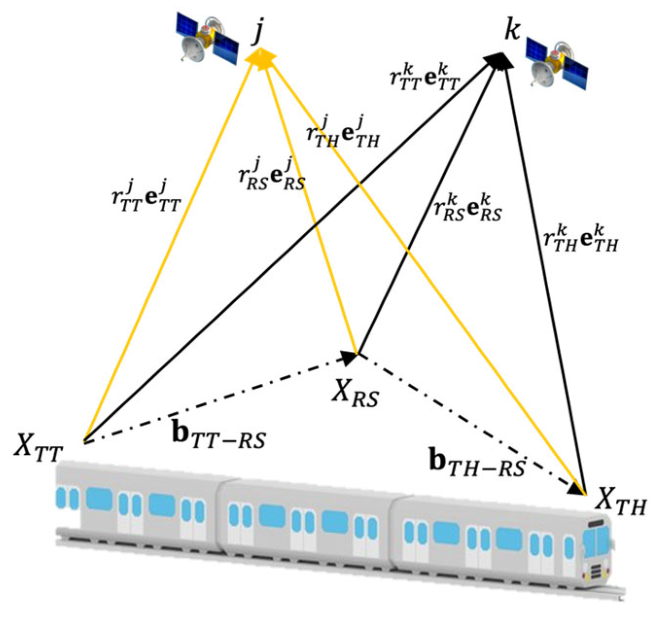
In practical scenarios, train lengths are typically smaller than 1000 m, which implies that the track slope difference between TH and TT is generally small, leading to a large inflation error, thereby adversely affecting train position determination, even though this influence is eliminated for the train length calculation. In pursuit of greater accuracy in train positioning, a dual DD baseline fusion algorithm (Dual DD algorithm) has been proposed. The Dual DD algorithm utilizes the ‘TH and RS’ DD baseline model and the ‘TT and RS’ DD baseline model, presented in Figure 5. These two DD baseline models run in parallel and follows a similar iterative procedure as Section 2.2 to correct the coarse odometer of TT (TH) in each baseline model. This algorithm aims to address the impact of track slope difference between the train head and tail. Then, only one odometer correction needs to be created in each DD baseline model. As a result, Equation (10) in each DD baseline model needs to be modified into (20).

$$\begin{array}{c}{\mathbf{D}\mathbf{D}}_{phi, \mathit{W}\mathit{L} }-{\mathbf{B}}^{\left(\mathit{n}\right)}{\mathbf{b}}^{\left(n\right)}={\mathbf{B}}^{\left(n\right)}\partial {\mathbf{X}}_{TH\left(TT\right)-RS}^{\left(n\right)}∆{\mathbf{s}}_{TH\left(TT\right)-RS}^{\left(n\right)}+\mu \end{array},$$

(20)

where $∆{\mathbf{s}}^{\left(n\right)}={\left[\begin{array}{c}\begin{array}{c}{∆s^{\left(n\right)}}_{TH\left(TT\right)}\left(t\right)\end{array}\end{array}\right]}_{1\times 1}$, ${\mathbf{B}}^{\left(n\right)}={\left[{\displaystyle \frac{1}{2}}\left(\left({\mathit{e}}_{TH\left(TT\right)}^k-{\mathit{e}}_{TH\left(TT\right)}^j)+{(\mathit{e}}_{RS}^k-{\mathit{e}}_{RS}^j\right)\right)\right]}_{m\times 3}$, ${\mathbf{b}}^{\left(n\right)}={\left[{\mathbf{X}}_{TH}\left({s^{\left(n\right)}}_{TH\left(TT\right)}\left(t\right)\right)-{\mathbf{X}}_{TT}\left({s^{\left(n\right)}}_{RS}\left(t\right)\right)\right]}_{3\times 1}$; $\partial {\mathbf{X}}^{\left(n\right)}={{\left[\begin{array}{cc}{{\displaystyle \frac{\partial {\mathbf{X}}_{TH\left(TT\right)}\left(s_{TH\left(TT\right)}\left(t\right)\right)}{\partial s_{TH\left(TT\right)}\left(t\right)}}}_{3\times 1}& ,{-{\displaystyle \frac{\partial {\mathbf{X}}_{RS}\left(s_{RS}\left(t\right)\right)}{\partial s_{RS}\left(t\right)}}}_{3\times 1}\end{array}\right]}_{3\times 2}=\left[\begin{array}{c}{\displaystyle \frac{\partial {\mathbf{X}}_{TH\left(TT\right)}\left(s_{TH\left(TT\right)}\left(t\right)\right)}{\partial s_{TH\left(TT\right)}\left(t\right)}}\end{array}\right]}_{3\times 1}$. The odometer corrections of train head and train tail, therefore, can be obtained accurately from these two DD baseline models when atmospheric error can be ignored. These corrected odometer values can then be used to obtain the corresponding train coordinates in the track database, and the train length information.

Given that the Dual DD algorithm utilizes a long-baseline model, ensuring the reliability of the measurements from the selected station at all times can be challenging. The cross-checking function is therefore introduced and illustrated in Figure 6. In this scheme, the Dual DD algorithm is first employed to derive the corrected odometers and position of both the TH and TT, as well as train length information. Additionally, the Single DD algorithm is utilized to calculate a redundant train length, which is then compared to the train length computed by the Dual DD algorithm to evaluate the status of the selected reference stations (RSs). In case the residual atmospheric error in the measurements exceeds a predetermined threshold, the selected RS is deemed unhealthy.

4. Simulation

The aim of using simulation data was to specifically investigate and tackle the problem of noise propagation caused by geometric factors on the algorithms, with the premise of static train. This section covers the simulation setup requirements and presents the numerical outcomes of the algorithms’ performance.

4.1. Database Setup and Measurement Simulation

First, we construct a railway database based on the light rail in Hong Kong. Based on Google Earth, we obtained the vector file composed of the track points on the part of the MTR Tuen Ma Line. The yellow marks in Figure 7 shows three stations of the MTR Tuen Ma line. By fitting these sample points, a railway trajectory equation can be constructed:

$$y=3.130936x^2-139.932319x+1677.480181,$$

(21)

where $y$ denotes the longitude and $x$ represents the latitude. The trajectory of the railway is illustrated in Figure 8. The latitude loop [22.3941:0.0000005:22.9] with the unit of degree is substituted into Equation (21) to obtain the corresponding longitude loop, where “[]” is a dataset, with the start point, interval, and end point placed in order. Furthermore, with the ellipsoidal height set unchanged along the train track as 35 m, the latitude and longitude dataset of the railway trajectory can be transformed into the ECEF position dataset $\left(x,y,z\right)$ according to the Earth ellipsoid model. The dataset for mileage computation is constructed by accumulating the distances between arbitrary pairs of points from a 12 km ECEF point set. Specifically, the mileage value for a given point is determined by summing up the distances between that point and all previous points in the dataset. For instance, if the distances between any two points in the first three entries of ECEF points are all 0.1 m, then the odometer value of the third set would be 0.2 m. The first ECEF point in the dataset is assigned a mileage value of 0 km. Then, we can obtain a track database consisting of ECEF position information and corresponding mileage value, presented in Figure 9.

We downloaded the brdc3350.21n (1st DEC 2021) broadcast GPS ephemeris navigation file from Wuhan University (http://www.igs.gnsswhu.cn (accessed on 4 April 2024), through which the satellite information can be obtained. The period starts from 10:00 AM, lasting 1000 epochs with a sample rate of 1 hz. The elevation angel cutoff was set as 10°, and the available satellites can be viewed through a skyplot (Figure 10), where the asterisk represents the satellite.

The location of the reference station in the Dual DD algorithm is fixed at a latitude of 22.65 and a longitude of 114.4. Simulated carrier phase measurements for both L1 and L2 frequencies are generated based on the geometric distance between the ground receivers (train head, train tail, and reference stations) and the satellites, with a noise level of sigma 0.0067 m added. However, common measurement errors such as troposphere delay, ionosphere delay, and satellite orbit error have not been taken into consideration in this simulation. In line with our research focus on noise-related issues, the carrier measurements are assumed to exclude the integer ambiguity. It is important to note that, for the sake of simplicity, the cycle slips of the carrier measurements have not been considered in this simulation.

The true odometer subset of the train tail is set to begin at 403.9 m of the track mileage dataset, with a train speed of 50 m/s over 1000 epochs. Assuming the train to be a rigid body and considering its length to be 600 m, the corresponding subset of the true odometer of the train head is determined.

After that, the error odometer subset of train tail is simulated by adding a 0.05 m/s error on true subset, followed by the error subset of train head establishment with a 0.02 m/s error.

The diagram of simulation is presented in Figure 11.

4.2. Verification of Improved Coefficient Matrix

The objective of this section is to validate the enhancement to the DD baseline precision achieved by the proposed coefficient matrix in contrast to that of Neri, as discussed in Section 2.1. As shown in Figure 12, the verification is based on the measurements and data based on the ‘train head and train tail’ DD baseline model. Simulated measurements were generated using only the geometric distance between the ground and satellites without any added noise.

The results show the derived matrix B can perform better than ${\mathbf{B}}_{neri}$ for the DD baseline model with a much smaller difference in both sides of equation under the same train length setting in these two experiments.

4.3. Numerical Result of Single DD Algorithm

Figure 13 presents the comparison between DOP and SIF in the Single DD algorithm. The highly level of consistency between SIF and DOP further verifies the deduction from ‘vector analysis’ model, that noise amplification is directly related to the difference in track slope between train head and train tail. The result also verifies that the $\mathbf{B}$ matrix is not an essential factor influencing the value of DOP, as the ratio of SIF and the DOP varies in a small scale with the same measurement number. Furthermore, only a small jump in the DOP can be seen with the change in available satellite number from epoch 539 to 540, in which the measurement number change would influence matrix $\mathbf{B}$. Overall, the straightening of the track is associated with a smaller difference in track slope between TH and TT, resulting in an increased DOP/SIF value.

Following the procedures in Section 2.2, the results of Single DD algorithm can be obtained subsequently. These results align with the deduction presented in Section 3. Based on Figure 14 and Figure 15, a direct correlation between the DOP/SIF value and odometer errors can be observed. Higher DOP/SIF values lead to increased errors in the odometer fix, resulting in comparable impacts on train position estimation up to tens of meters. However, this type of error exhibits a consistent trend between the train head and train tail, allowing for the cancelation of most of the errors in train length calculation, as shown in Figure 16.

4.4. Numerical Result of Dual DD Algorithm

The results of DOP and SIF both demonstrate the low noise sensitivity of the coefficient matrix, presented in Figure 17. This confirmed the significant advantage of the Dual DD algorithm in terms of train odometer correction and position estimation, presented in Figure 18 and Figure 19. The accuracy achieved was at the decimeter level. However, the positional error of the train head and tail showed an uneven distribution of accuracy along the three directions due to different rates of change in the three-directional coordinates with respect to track mileage, as depicted in Figure 20. Since the acquisition of train coordinates is based on the odometer of the track database, a low rate of change in the coordinates results in higher coordinate accuracy. The train length computation using the Dual DD algorithm showed similar performance to that of the Single DD algorithm, as shown in Figure 21.

4.5. Numerical Result of Train Length Cross Checking

If the chosen reference stations (RSs) do not contain significant residual errors, the calculated difference in train length between the Single DD algorithm and the Dual DD algorithm remains stable and follows a normal distribution with a mean of 0.0005 and a standard deviation of 0.0001 m given the measurement noise set by Section 4.1, as presented in Figure 22. However, in real-world scenarios, atmospheric disturbances may dominate the position error in the medium or long baseline model, and a suitable station may not always be available. In such cases, if the computed train length difference exceeds a predefined threshold, it may be appropriate to not use the measurements at that epoch and instead use the coarse odometer that has been corrected for accumulated error with the aid of previous reliable measurements based on Equation (14).

5. Conclusions

The paper proposes a dual DD scheme to concurrently provide train location and integrity safety information. The Dual DD algorithm eliminates the impact of track slope difference that existed in the Single DD algorithm and obtains precise odometer corrections and train location, while the Single DD algorithm is employed for redundant train length calculation. Then, the redundancy is compared to the train length computed through the Dual DD algorithm to verify the status of selected stations.

To verify the effectiveness of the proposed models, a series of numerical simulation results were carried out on the MTR Tuen Ma line. The Dual DD algorithm effectively reduces the impact of track slope differences between the train head and tail. Under a carrier phase measurement noise level of 0.0067 m, simulation results show that the Dual DD algorithm improves the accuracy of train location estimation by up to an order of magnitude compared to the Single DD algorithm. Assuming a negligible atmospheric delay, the difference in computed train integrity between the Single DD and Dual DD algorithms follows a normal distribution with a mean of 0.0005 m and a standard deviation of 0.0001 m, thereby validating the reliability of the cross-checking function. Consequently, the integration of the Dual DD algorithm with the cross-checking function represents a critical step toward the practical application of the DD baseline model at the ETCS Level 3.

References

1. Basile, D.; Beek, M.H.; Ferrari, A.; Legay, A. Modelling and analysing ERTMS L3 moving block railway signalling with Simulink and Uppaal SMC. In Proceedings of the Formal Methods for Industrial Critical Systems: 24th International Conference, Amsterdam, The Netherlands, 30–31 August 2019; pp. 1–21. [Google Scholar]
2. Biagi, M.; Carnevali, L.; Paolieri, M.; Vicario, E. Performability evaluation of the ERTMS/ETCS–Level 3. Transp. Res. Part C Emerg. Technol. 2017, 82, 314–336. [Google Scholar] [CrossRef]
3. Li, S.H.; Cai, B.; Xu, A.; Shangguan, W.; Wen, Y.H.; Wang, J. Autonomous-Positioning information aided train integrity detection risk analysis method. J. Southwest Jiaotong Univ. 2017, 52, 886–892. [Google Scholar]
4. Jiang, W.; Liu, Y.; Cai, B.; Rizos, C.; Wang, J.; Jiang, Y. A new train integrity resolution method based on online carrier phase relative positioning. IEEE Trans. Veh. Technol. 2020, 69, 10519–10530. [Google Scholar] [CrossRef]
5. Zafar, N.A.; Khan, S.A.; Araki, K. Towards the safety properties of moving block railway interlocking system. Int. J. Innov. Comput. Inf. Control. 2012, 8, 5677–5690. [Google Scholar]
6. Furness, N.; Van Houten, H.; Arenas, L.; Bartholomeus, M. ERTMS level 3: The game-changer. IRSE News 2017, 232, 2–9. [Google Scholar]
7. Palumbo, M. Railway Signaling Since the Birth to ERTMS; Railway signaling Europe: London, UK, 2013. [Google Scholar]
8. Scholten, H.; Westenberg, R.; Schoemaker, M. Sensing train integrity. In Proceedings of the SENSORS 2009 IEEE, Christchurch, New Zealand, 25–28 October 2009; pp. 669–674. [Google Scholar]
9. Neri, A.; Rispoli, F.; Salvatori, P. An analytical assessment of a GNSS-based train integrity solution in typical ERTMS level 3 scenarios. In Proceedings of the European Navigation Conference, Bordeaux, France, 7–10 April 2015. [Google Scholar]
10. Rispoli, F.; Castorina, M.; Neri, A.; Filip, A.; Di Mambro, G.; Senesi, F. Recent progress in application of GNSS and advanced communications for railway signaling. In Proceedings of the 2013 23rd International Conference Radioelektronika (RADIOELEKTRONIKA), Pardubice, Czech Republic, 16–17 April 2013; pp. 13–22. [Google Scholar]
11. Bai, S.; Jiang, Y.; Sun, W.; Shao, W. Modified Two-Dimensional Coverage Analysis Method Considering Various Perturbations. IEEE Trans. Aerosp. Electron. Syst. 2023, 60, 2763–2777. [Google Scholar] [CrossRef]
12. Bai, S.; Zhang, Y.; Jiang, Y. Minimum-observation Method for Rapid and Accurate Satellite Coverage Prediction. GPS Solut. 2022, 26, 110. [Google Scholar] [CrossRef]
13. Jiang, W.; Liu, Y.; Liu, D.; Cai, B.; Wang, J. Train integrity monitoring based on GNSS moving-baseline approach. In Proceedings of the 11th International Conference on Modelling, Identification and Control (ICMIC 2019), Tianjin, China, 13–15 July 2019; Volume 582, pp. 653–662. [Google Scholar]
14. Lauer, M.; Stein, D. A train localization algorithm for train protection systems of the future. IEEE Trans. Intell. Transp. Syst. 2014, 16, 970–979. [Google Scholar] [CrossRef]
15. Neri, A.; Capua, R.; Salvatori, P. Track Constrained RTK-like Positioning for Railway Applications. Navig. J. Inst. Navig. 2018, 65, 335–352. [Google Scholar] [CrossRef]
16. Neri, A.; Palma, V.; Rispoli, F.; Vegni, A.M. Track constrained PVT estimation based on the double-difference technique for railway applications. In Proceedings of the 21st European Signal Processing Conference (EUSIPCO 2013), Marrakech, Morocco, 9–13 September 2013; pp. 1–5. [Google Scholar]
17. Neri, A.; Rispoli, F.; Salvatori, P.; Vegni, A.M. A train integrity solution based on GNSS double-difference approach. In Proceedings of the 27th International Technical Meeting of The Satellite Division of the Institute of Navigation (ION GNSS+ 2014), Tampa, FL, USA, 8–12 September 2014; pp. 34–50. [Google Scholar]
18. Gerlach, K.; Hörste, M.M. A precise digital map for GALILEO-based train positioning systems. In Proceedings of the 2009 9th International Conference on Intelligent Transport Systems Telecommunications (ITST), Lille, France, 20–22 October 2009; pp. 343–347. [Google Scholar]
19. Heirich, O.; Robertson, P.; Strang, T. RailSLAM-Localization of rail vehicles and mapping of geometric railway tracks. In Proceedings of the IEEE International Conference on Robotics and Automation, Karlsruhe, Germany, 6–10 May 2013; pp. 5212–5219. [Google Scholar]
20. Nash, A.; Huerlimann, D.; Schütte, J.; Krauss, V.P. Railml a standard data interface for railroad applications. In WIT Transactions on The Built Environment; WIT Press: Southampton, UK, 2004; p. 74. [Google Scholar]
21. Zhu, J. Calculation of geometric dilution of precision. IEEE Trans. Aerosp. Electron. Syst. 1992, 28, 893–895. [Google Scholar]
22. Sharp, I.; Yu, K.; Guo, Y.J. GDOP analysis for positioning system design. IEEE Trans. Veh. Technol. 2009, 58, 3371–3382. [Google Scholar] [CrossRef]
23. Strang, G. The fundamental theorem of linear algebra. Am. Math. Mon. 1993, 100, 848–855. [Google Scholar] [CrossRef]
Figure 1. Single DD algorithm scheme.
Electronics 14 01591 g001
Figure 2. Data flow of iteration process.
Electronics 14 01591 g002
Figure 3. Situation A and B in Case 1.
Electronics 14 01591 g003
Figure 4. Situation A and B in Case 2.
Electronics 14 01591 g004
Figure 5. Dual DD algorithm.
Electronics 14 01591 g005
Figure 6. Cross-checking function.
Electronics 14 01591 g006
Figure 7. Stations of MTR Tuen Ma Line.
Electronics 14 01591 g007
Figure 8. The trajectory of the railway projected in two-dimensional space.
Electronics 14 01591 g008
Figure 9. The track database setting.
Electronics 14 01591 g009
Figure 10. Skyplot of selected satellites.
Electronics 14 01591 g010
Figure 11. Flowchart of simulation setup.
Electronics 14 01591 g011
Figure 12. Verification of improved coefficient matrix.
Electronics 14 01591 g012
Figure 13. Comparison between DOP and SIF.
Electronics 14 01591 g013
Figure 14. Odometer correction of train head (left) and train tail (right).
Electronics 14 01591 g014
Figure 15. Position error of train head (left) and train tail (right).
Electronics 14 01591 g015
Figure 16. Error of train length.
Electronics 14 01591 g016
Figure 17. DOP and SIF of ‘train head and reference station’ baseline model.
Electronics 14 01591 g017
Figure 18. Odometer correction of train head (left) and train tail (right).
Electronics 14 01591 g018
Figure 19. Position error of train head (left) and train tail (right).
Electronics 14 01591 g019
Figure 20. Coordinate change rate with track mileage.
Electronics 14 01591 g020
Figure 21. Error of train length.
Electronics 14 01591 g021
Figure 22. Train length difference.
Electronics 14 01591 g022
Disclaimer/Publisher’s Note: The statements, opinions and data contained in all publications are solely those of the individual author(s) and contributor(s) and not of MDPI and/or the editor(s). MDPI and/or the editor(s) disclaim responsibility for any injury to people or property resulting from any ideas, methods, instructions or products referred to in the content.