Nonlinear Observer Based on an Integrated Active Controller Applied to a Tractor with a Towed Implement System

Abstract

In this paper, a methodological framework employing an observer-based nonlinear controller is presented for controlling the lateral velocity of a farm tractor, as well as the yaw velocity of the agricultural implement. This approach relies on measurements obtained from sensors installed on a modern farm tractor, including lateral and longitudinal accelerations, longitudinal velocity, yaw rate, steering angle, and the differential yaw rate between the farm tractor and the implement. The nonlinear observer estimates the longitudinal and lateral velocities of the vehicle, as well as the roll dynamics of the implement, and ensures the exponential convergence of the observed variables. The control objective is formulated to ensure error feedback control, guaranteeing accurate tracking of the lateral velocity and yaw rate of the farm tractor and implement, following the reference patterns for these variables. The reference system is modeled as an “ideal” tractor operating without attachments. To evaluate the proposed controller’s performance, two test maneuvers were conducted. The first test involved the classic U-turn maneuver, commonly executed by tractors, while the second was a double-step maneuver, a standard in ground vehicle testing. Both maneuvers were simulated using MATLAB–Simulink to evaluate the controller’s effectiveness and robustness against parameter variations.

1. Introduction

Meeting the global demand for food requires a substantial increase in sustainable agricultural productivity. This goal can be achieved by improving the efficiency of fundamental agricultural operations, such as plowing, planting, fertilizing, and harvesting, through the automation of agricultural machinery [1]. The application of advanced technologies reduces operating time, energy consumption, and input usage, thereby lowering production costs and improving the overall efficiency of farming activities [2]. Moreover, increased precision in field operations minimizes overlap, reduces crop damage, and mitigates the adverse effects of intensive agrochemical application.

Automation technologies for agricultural machinery, particularly farm tractors, have been a focal point of research in recent decades. Early advances in short-range sensing methods were employed, including vision-based guidance systems [3], while the advent of GPS technology enabled more precise guidance solutions for agricultural vehicles [4,5,6]. These innovations have facilitated the development of advanced controllers capable of navigating farm vehicles along complex trajectories [7,8]. However, many existing guidance systems are limited to tractor-mounted sensors, even though agricultural implements are responsible for most field operations [9,10]. Recent studies have explored control systems for tractor–implement combinations, including automatic steering controllers based on kinematic models [11,12] and LQR controllers for tracking and control [13].

Despite these advances, much of the existing technology focuses on autonomous tractors. This paper proposes a novel approach for non-autonomous farm tractors, leveraging “by-wire” systems—namely, steer-by-wire and brake-by-wire systems—that enable greater flexibility in the design of control laws. These systems decouple mechanical connections, allowing the integration of actuators like Rear Torque Vectoring (RTV) and Active Front Steering (AFS) to enhance vehicle stability and compensate for external disturbances [14,15,16,17]. Such innovations are particularly beneficial for integrating control strategies tailored to tractor–implement systems.

This work presents a significant advancement in agricultural vehicle control, addressing multiple challenges that have not been previously proposed or integrated in tractors, with the main contributions outlined as follows:

1.

The proposed controller integrates AFS and RTV to account for parameter variations while addressing the challenge of unmeasured state variables, such as lateral velocity and roll dynamics.

2.

A nonlinear observer-based integrated active controller is designed for a tractor with a towed implement system. The observer reconstructs unmeasured states by deriving them from measurable quantities, including accelerations, longitudinal velocity, yaw rate, and steering angle.

3.

The inclusion of Pacejka’s formula for tire dynamics provides a significant improvement in modeling nonlinear behaviors.

4.

The controller’s performance is validated through two standard test maneuvers: the classic U-turn and the double-step maneuver, commonly used in ground vehicle testing.

5.

MATLAB–Simulink simulations are conducted to demonstrate the effectiveness and applicability of the proposed approach.

Maintaining precise control over the orientation of a tractor–implement system is crucial for enhancing agricultural efficiency, reducing overlap in operations, and minimizing the wastage of resources. The emergence of by-wire systems has enabled the replacement of traditional mechanical and hydraulic components with flexible electronic control systems. This flexibility facilitates the design of advanced controllers, such as dual servomotor-based steer-by-wire mechanisms, which decouple the driver input from the wheel assembly, enhancing the system’s ability to respond to external disturbances. Similar innovations, such as brake-by-wire subsystems and active differentials, further improve vehicle stability by applying active yaw moments [18,19,20,21,22].

Previous research on lateral velocity observers has predominantly focused on nonlinear techniques, often neglecting roll angular velocity. Studies have incorporated friction adaptability [23], evaluated Dugoff’s tire models [24], and explored sliding mode techniques [25]. Reduced-order nonlinear observers [26] and switched multiple nonlinear observers [27] have also been investigated for stability and friction estimation. Additionally, nonlinear tracking controllers with extended state observers have demonstrated potential for active vehicle suspensions, ensuring comfort and stability under dynamic constraints [28].

Moreover, recent advances in nonlinear control have introduced more robust sliding mode strategies across a variety of engineering applications. For instance, fixed-time sliding mode controllers with enhanced disturbance rejection have been developed in [29,30,31], where control frameworks were designed to ensure rapid convergence despite nonlinearities and external disturbances. In the case of finite-time sliding mode controllers, further improvements in compensation capability have been demonstrated in [32,33], particularly for underactuated marine systems subject to asymmetric input saturation. Additionally, gain-adaptive sliding mode control schemes have been explored in [34], where the adaptability of the controller gains ensures robustness in the presence of dynamic uncertainties. While these methods are tailored for diverse systems such as NPC converters, robotic manipulators, marine vehicles, and automotive actuators, the underlying control principles—namely, fast convergence, disturbance rejection, and robustness to parameter variations—are highly relevant and have inspired the design of the robust controller proposed in this work.

The proposed work builds on these advances by addressing the unique challenges of tractor–implement systems in agricultural applications.

This paper is organized as follows: Section 2 introduces the mathematical model for the farm tractor–implement system. Section 3 details the design of a nonlinear observer. Section 4 outlines the development of the dynamic controller, while Section 5 presents its validation through simulation results. Lastly, the conclusions are summarized.

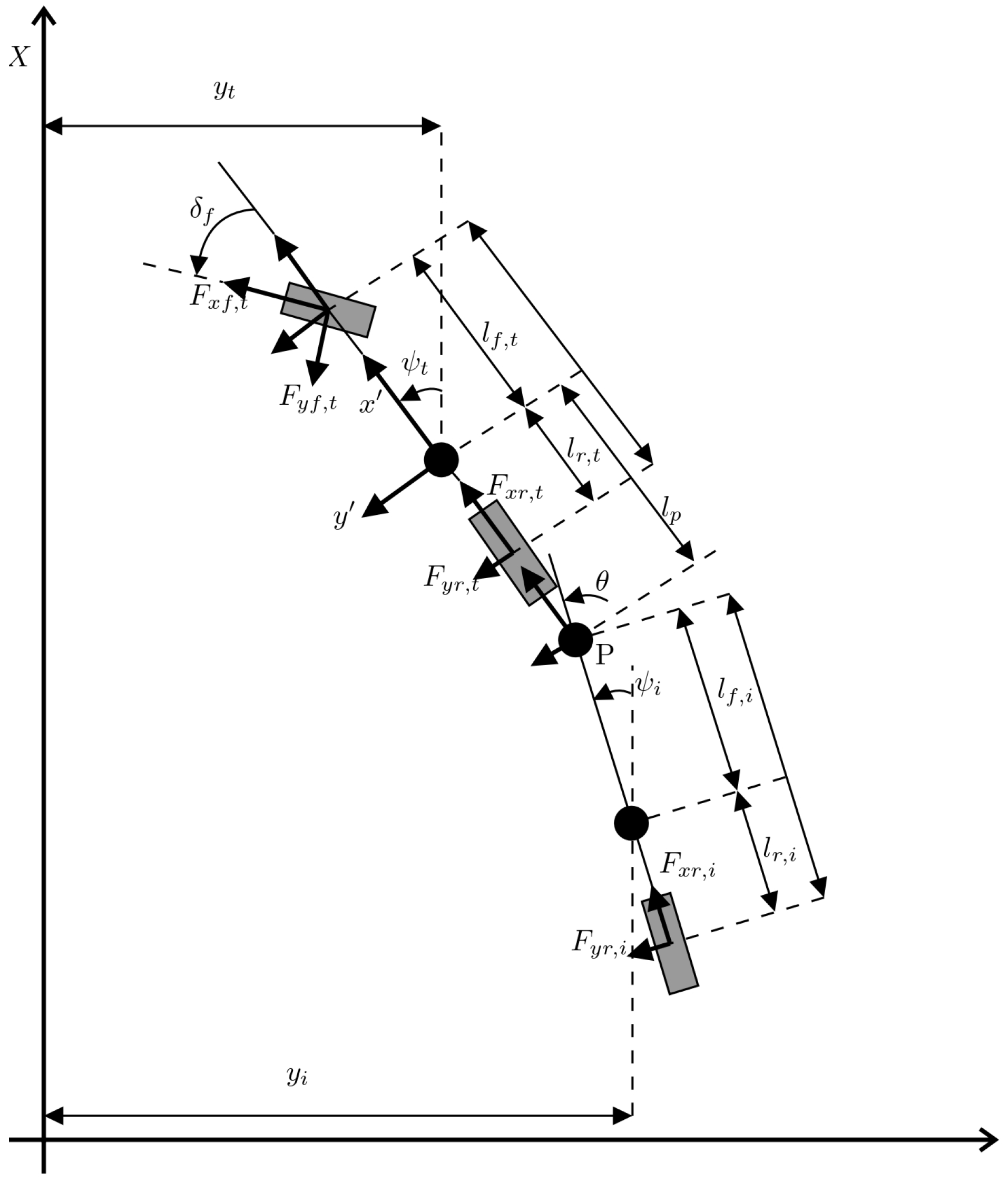
2. Mathematical Model

This section introduces the mathematical model for a tractor–implement system. The model assumes that the agricultural vehicle behaves as a rigid body interacting with the ground through its tires. Additionally, the farm tractor is linked to an implement via the hitch point, which serves as the reference point, as shown in Figure 1. Figure 2 provides a schematic representation of the external forces acting upon the coupled tractor–implement system. The mathematical model presented in this paper includes longitudinal/lateral velocity and yaw rate variables for both the tractor and the implement. Furthermore, the model considers the angle differences between the tractor’s and implement’s yaw rates. Traction and rolling resistance forces are neglected. These dynamics are represented using the so-called single-track or bicycle model, as depicted in Figure 1 and Figure 2.

In recent years, engineers have incorporated new technologies, such as steer-by-wire (SBW), into agricultural vehicles, including Active Front Steering (AFS) and Rear Torque Vectoring (RTV). The AFS system acts on the front tires, increasing the steering angle ${\delta }_c$, while the RTV applies negative longitudinal forces $M_z$, resulting in a yaw moment. These two control actions are decoupled, meaning they do not interfere with each other, particularly in rear-wheel-drive vehicles.

To analyze the complex dynamics of the farm tractor and the towed implement system, and evaluate the performance of the proposed dynamic controller, an accurate simulation model is utilized. For this, the single-track model is considered; see Figure 1 and Figure 2.

The mathematical model describing the farm tractor’s dynamics incorporates its longitudinal, lateral, and yaw velocities (see Appendix A for the list of variables), as follows:

$$\begin{array}{cc}\hfill m_t\left({\dot{v}}_{x,t}-v_{y,t}{\mathit{\omega }}_{z,t}\right)=& F_{xf,t}+F_{xr,t}=m_t{a}_{x,t}\hfill \\ \hfill m_t\left({\dot{v}}_{y,t}+v_{x,t}{\mathit{\omega }}_{z,t}\right)=& F_{yf,t}+F_{yr,t}+F_{yp,t}\hfill \\ \hfill J_{z,t}{\dot{\mathit{\omega }}}_{z,t}=& l_{f,t}{F}_{yf,t}-l_{r,t}{F}_{yr,t}-l_p{F}_{yp,t}\hfill \end{array}$$

(1)

In this context, $m_t$ denotes the mass of the tractor, and $J_{z,t}$ its moment of inertia with respect to the yaw axis. The distances $l_{f,t}$ and $l_{r,t}$ define the position of the center of gravity (CG) relative to the front and rear axles, while $l_p$ defines the spacing between the hitch point and the CG. The front wheel steering angle is indicated by ${\delta }_f$. The velocity components $v_{x,t}$ and $v_{y,t}$ correspond to the longitudinal and lateral velocities at the tractor’s CG, and ${\mathit{\omega }}_{z,t}$ refers to the yaw rotational rate. The longitudinal forces acting on the front and rear tires are denoted by $F_{x,f,t}$ and $F_{x,r,t}$, while $F_{y,f,t}$ and $F_{y,r,t}$ represent the lateral tire forces. The interaction between the implement and the tractor is represented by the lateral force $F_{y,p,t}$.

To analyze the implement’s dynamics, we assume that the tractor’s velocity at its center of gravity (CG) influences the implement’s CG through the hitch connection. The resulting kinematic relationships are described by the following equations:

$$\begin{array}{cc}\hfill v_{x,i}& =v_{x,t}cos\left(\theta \right)-\left(v_{y,t}-l_p{\mathit{\omega }}_{z,t}sin\left(\theta \right)\right)\hfill \\ \hfill v_{y,i}& =v_{x,t}sin\left(\theta \right)+\left(v_{y,t}-l_p{\mathit{\omega }}_{z,t}\right)cos\left(\theta \right)-l_{f,i}{\mathit{\omega }}_{z,i}\hfill \end{array}$$

here, $v_{x,i}$ and $v_{y,i}$ denote the implement’s longitudinal and lateral velocities, respectively, while ${\mathit{\omega }}_{z,i}$ represents its yaw rate. The variable $\theta$ defines the angle between the directions of the tractor and the implement, and $l_{f,i}$ specifies the distance from the implement’s CG to its front.

Considering that the longitudinal velocities of both the tractor and the implement are equal ($v_{x,t}=v_{x,i}$), since they are mechanically attached, the analysis focuses solely on the implement’s lateral velocity dynamics.

$$\begin{array}{cc}\hfill {\dot{v}}_{y,i}& ={\dot{v}}_{x,t}sin\left(\theta \right)+v_{x,t}cos\left(\theta \right)\dot{\theta }+\left({\dot{v}}_{y,t}-l_p{\dot{\mathit{\omega }}}_{z,t}\right)cos\left(\theta \right)-\left(v_{y,t}-l_p{\mathit{\omega }}_{z,t}\right)sin\left(\theta \right)\dot{\theta }\hfill \\ \hfill & -l_{f,i}{\dot{\mathit{\omega }}}_{z,i}\hfill \end{array}$$

(2)

where

$$\dot{\theta }={\mathit{\omega }}_{z,t}-{\mathit{\omega }}_{z,i}$$

However, in practical terms, the following assumptions can be considered:

Assumption 1. 

The steering angle ${\delta }_f$ is assumed to be small.

Assumption 1 is considered reasonable because, at typical farm operating velocities below 7.5 m/s, the lateral load transfer has a minimal effect on the overall cornering force when small steering angles are involved. Consequently, this assumption also suggests that the heading angle $\theta$ remains within a small range.

Assumption 2. 

The angle θ is considered small.

Assumption 2, which considers a small heading angle $\theta$, is valid when the model is applied to tracking smooth trajectories that exhibit minor changes in heading along a straight path. This assumption holds when designing a path-following controller with small variations in the tractor’s steering direction ${\delta }_f$. However, if the model is used in more general scenarios or with abrupt changes in ${\delta }_f$, the small-angle assumption for $\theta$ may no longer be appropriate.

Due to Assumptions 1 and 2, and without loss of generality, we set $sin\theta =0$ and $cos\theta =1$. As a result, the lateral velocity dynamics of the implement, as shown in Equation (2), is simplified: [35]

$${\dot{v}}_{y,i}=v_{x,t}({\mathit{\omega }}_{z,t}-{\mathit{\omega }}_{z,i})+{\dot{v}}_{y,t}-l_p{\dot{\mathit{\omega }}}_{z,t}-l_{f,i}{\dot{\mathit{\omega }}}_{z,i}$$

(3)

Meanwhile, the yaw dynamics of the implement can be expressed as

$$J_{z,i}{\dot{\mathit{\omega }}}_{z,i}=l_{f,i}{F}_{yp,i}-l_{r,i}{F}_{yr,i}$$

(4)

where $l_{r,i}$ is the rear implement length, $J_{z,i}$ is the implement’s moment of inertia, $F_{yp,i}$ is the lateral force applied to the implement, and $F_{yr,i}$ is the lateral force generated by the implement’s rear tire.

The Tractive Force

The single-track model depicted in Figure 1 and Figure 2 is classified as a nonlinear system because the longitudinal/lateral forces acting on the front and rear tires of the farm tractor ($F_{xf,t},F_{xr,t},F_{yf,t},F_{yr,t}$) and the lateral force on the implement’s tires ($F_{yr,i}$) exhibit a nonlinear dependence on the slip angles of the front and rear tires of the tractor, as well as the rear tire angle of the implement [35].

$$\begin{array}{cc}\hfill {\alpha }_{f,t}& ={\delta }_f-(v_{y,t}+l_{f,t}{\mathit{\omega }}_{z,t})/v_{x,t}\hfill \\ \hfill {\alpha }_{r,t}& =-\left(v_{y,t}-l_{r,t}{\mathit{\omega }}_{z,t}\right)/v_{x,t}\hfill \\ \hfill {\alpha }_{r,i}& =-\left(v_{y,t}-l_p{\mathit{\omega }}_{z,t}-(l_{f,i}+l_{r,i}){\mathit{\omega }}_{z,i}\right)/v_{x,t}-\theta \hfill \end{array}$$

(5)

The road wheel angle ${\delta }_f$ is defined as the sum of the driver’s steering input ${\delta }_d$ and the AFS contribution ${\delta }_c$, where ${\delta }_d$ is assumed to be a continuously differentiable function over time.

The tire slip angle, ${\alpha }_{f,t}$, possesses specific characteristics, including a well-defined range with minimum and maximum limits, such that ${\alpha }_{f,t}=\pm {\alpha }_{f,t,\max }$. Moreover, it is considered an invertible function with respect to ${\alpha }_{f,t}$, within the range ${\alpha }_{f,t}\in [-{\alpha }_{f,t,\max },{\alpha }_{f,t,\max }]$.

The nonlinear behavior of the simplified model originates from the tire characteristics. This study employs the mathematical representation known as the simplified Pacejka formula:

$$\begin{array}{cc}\hfill F_{yf,t}\left({\alpha }_{f,t}\right)& =D_{f,t}sin\left(C_{f,t}arctan\left(B_{f,t}{\alpha }_{f,t}\right)\right)\hfill \\ \hfill F_{yr,t}\left({\alpha }_{r,t}\right)& =D_{r,t}sin\left(C_{r,t}arctan\left(B_{r,t}{\alpha }_{r,t}\right)\right)\hfill \\ \hfill F_{yr,i}\left({\alpha }_{r,t}\right)& =D_{r,i}sin\left(C_{r,i}arctan\left(B_{r,i}{\alpha }_{r,i}\right)\right)\hfill \end{array}$$

(6)

with $B_{i,j}$, $C_{i,j}$, $D_{i,j}$, where $i=f,r$ and $j=t,i$ are experimental parameters [36]. The coefficients $B_{i,j},C_{i,j},D_{i,j}$ play a crucial role in defining the nonlinear tire force characteristics. Specifically, the following apply:

$B_{i,j}$ (stiffness factor) affects the shape of the force–slip curve and determines how quickly the lateral force builds up as the slip angle increases.

$C_{i,j}$ (shape factor) influences the curvature of the response and controls the steepness of the transition from the linear to the nonlinear region.

$D_{i,j}$ (peak factor) represents the maximum lateral force that the tire can generate.

For agricultural vehicles, these parameters depend on several factors, including soil type, tire inflation pressure, and load conditions.

Similarly, to determine the lateral force at the hitch point $F_{yp,i}$, it is possible to consider the lateral velocity dynamics of the implement (3) and the lateral force generated by the implement’s rear tire.

$$F_{yp,i}=m_i({\dot{v}}_{y,i}+v_{x,t}{\mathit{\omega }}_{z,t})-F_{yr,i}$$

(7)

and under Assumptions 1 and 2, one obtains

$$F_{yp,t}=-F_{yp,i}$$

(8)

The front lateral tire force of the tractor, $F_{yf,t}({\delta }_d+{\delta }_c,v_y,{\mathit{\omega }}_z)$, is treated as an invertible function with respect to the AFS control input ${\delta }_c$. As a result, for a specific value $F_{yf,t,0}$, the equation $F_{yf,t}({\delta }_d+{\delta }_c,v_{y,t},{\mathit{\omega }}_{z,t})=F_{yf,t,0}$ yields a unique solution, expressed as follows:

$${\delta }_c=\left\{\begin{array}{cc}-{\delta }_d+{\displaystyle \frac{v_{y,t}+l_{f,t}{\mathit{\omega }}_{z,t}}{v_{x,t}}}+F_{yf,t}^{-1}\left(F_{yf,t,0}\right),\hfill & \hfill \mathrm{if}{\alpha }_{f,t}\in [-{\alpha }_{f,t,max},{\alpha }_{f,t,max}]\\ -{\delta }_d+{\displaystyle \frac{v_{y,t}+l_{f,t}{\mathit{\omega }}_{z,t}}{v_{x,t}}}\pm F_{yf,t,max}\hfill & \hfill \mathrm{otherwise}\end{array}\right\}$$

The lateral force $F_{y,f}({\delta }_d+{\delta }_c,v_y,{\mathit{\omega }}_z)$ is treated as an invertible function, allowing the definition of the control input as shown below:

$${∆}_f=F_{yf,t}({\delta }_d+{\delta }_c,v_{y,t},{\mathit{\omega }}_{z,t})-F_{yf,t}({\delta }_d,v_{y,t},{\mathit{\omega }}_{z,t}).$$

(9)

By substituting the control input ${∆}_f$ and incorporating the rear torque vector $M_z$ into the lateral velocity and yaw rate dynamics of the agricultural vehicle from Equation (1), as well as the dynamics of the implement from Equations (3) and (4), the tractor–implement system is rewritten as follows:

$$\begin{array}{cc}\hfill & m_t\left({\dot{v}}_{x,t}-v_{y,t}{\mathit{\omega }}_{z,t}\right)=F_{xf,t}+F_{xr,t}\hfill \\ \hfill & m_t\left({\dot{v}}_{y,t}+v_{x,t}{\mathit{\omega }}_{z,t}\right)=F_{yfd,t}+F_{yr,t}+F_{yp,t}+{∆}_f\hfill \\ \hfill & J_{z,t}{\dot{\mathit{\omega }}}_{z,t}=l_{f,t}{F}_{yfd,t}-l_{r,t}{F}_{yr,t}-l_p{F}_{yp,t}+l_{f,t}{∆}_f+M_z\hfill \\ \hfill & J_{z,i}{\dot{\mathit{\omega }}}_{z,i}=l_{f,i}{F}_{yp,i}-l_{r,i}{F}_{yr,i}\hfill \end{array}$$

(10)

Using (7) and (8) in (10), and performing some algebraic operations, we obtain

$$\begin{gathered} \begin{array}{cc}\hfill {\dot{v}}_{x,t}& =v_{y,t}{\mathit{\omega }}_{z,t}+{\displaystyle \frac{1}{m_t}}{a}_{x,t}\hfill \end{array} \\ \left(\begin{array}{c}{\dot{v}}_{y,t}\\ {\dot{\mathit{\omega }}}_{z,t}\\ {\dot{\mathit{\omega }}}_{z,i}\end{array}\right)={\displaystyle \frac{1}{D}}\left(\begin{array}{ccc}{a}_{1,1}& a_{1,2}& a_{1,3}\\ a_{2,1}& a_{2,2}& a_{2,3}\\ a_{3,1}& a_{3,2}& a_{3,3}\end{array}\right)\left(\begin{array}{c}{f}_1\\ f_2\\ f_3\end{array}\right) \end{gathered}$$

(11)

where

$$\begin{array}{cc}\hfill D& =m_t{m}_i\left(l_p^2{J}_{z,i}+l_{f,i}^2{J}_{z,t}\right)+J_{z,t}{J}_{z,i}m\hfill \end{array}$$

(12)

and

$$\begin{array}{cc}\hfill m& =m_t+m_i\hfill \\ \hfill a_{1,1}& =(J_{z,i}{l}_p^2+J_{z,t}{l}_{f,i}^2)m_i+J_{z,i}{J}_{z,t}\hfill \\ \hfill a_{1,2}& =J_{z,i}{l}_p{m}_i\hfill \\ \hfill a_{1,3}& =l_{f,i}{J}_{z,t}{m}_i\hfill \\ \hfill a_{2,1}& =l_p{J}_{z,i}{m}_i\hfill \\ \hfill a_{2,2}& =l_{f,i}^2{m}_t{m}_i+J_{z,i}m\hfill \\ \hfill a_{2,3}& =-l_p{l}_{f,i}{m}_i{m}_t\hfill \\ \hfill a_{3,1}& =l_{f,i}{J}_{z,t}{m}_i\hfill \\ \hfill a_{3,2}& =-l_p{l}_{f,i}{m}_i{m}_t\hfill \\ \hfill a_{3,3}& =l_p^2{m}_t{m}_i+J_{z,t}m\hfill \end{array}$$

(13)

and

$$\begin{array}{cc}\hfill f_1& =-m{v}_{x,t}{\mathit{\omega }}_{z,t}+F_{yfd,t}+F_{yr,t}+F_{yr,i}+{∆}_f\hfill \\ \hfill f_2& =l_p{m}_i{v}_{x,t}{\mathit{\omega }}_{z,t}+l_{f,t}{F}_{yfd,t}-l_{r,t}{F}_{yr,t}-l_p{F}_{yr,i}+l_{f,t}{∆}_f+M_z\hfill \\ \hfill f_3& =l_{f,i}{m}_i{v}_{x,t}{\mathit{\omega }}_{z,t}-(l_{f,t}+l_{f,i})F_{yr,i}\hfill \end{array}$$

(14)

3. Nonlinear Observer Design

Lateral velocity $v_{y,t}$ is typically not measured directly. In the following, it is assumed that $a_{x,t},a_{y,t},{\mathit{\omega }}_{z,t},v_{x,t}$ are measurable. This assumption is reasonable for modern farm tractors [14,15,16,17], as they are generally equipped with the required sensors.

Assumption 3. 

The yaw angular velocity ${\mathit{\omega }}_{z,t}$ is assumed to remain bounded at all time $t\ge t_0$, i.e., $|{\mathit{\omega }}_{z,t}|\le {\mathit{\omega }}_{z,t,\mathit{max}}$.

Assumption 3 is physically reasonable; since the farm tractor is a finite energy system, the maximal yaw angular velocity remains bounded. In what follows, we derive an observer for which, for $|{\mathit{\omega }}_{z,t}|>0$ and under Assumption 3, the nonlinear observer guarantees that the estimation error converges to zero as time approaches infinity. Additionally, under Assumption 3, it should be noted that ${\mathit{\omega }}_{z,t}$ can pass through zero during a maneuver but cannot remain zero for a finite duration unless the vehicle moves in a perfectly straight line. In such cases, estimating the lateral velocity $v_{y,t}$ is no longer required.

Theorem 1. 

Under Assumption 3, and with $|{\mathit{\omega }}_{z,t}|>0$, and the signals ${\mathit{\omega }}_{z,t},v_{x,t},a_{x,t}$ being measurable, the nonlinear observer

$$\begin{array}{cc}\hfill {\dot{\widehat{v}}}_{x_t}& =v_{y,t}{\mathit{\omega }}_{z,t}+{\displaystyle \frac{1}{m_t}}{a}_{x,t}+k_{o,1}(v_{x,t}-{\widehat{v}}_{x,t})\hfill \\ \hfill {\dot{\widehat{v}}}_{y,t}& ={\displaystyle \frac{1}{D}}\left(a_{1,1}{\widehat{f}}_1+a_{1,2}{\widehat{f}}_2+a_{1,3}{\widehat{f}}_3\right)+k_{o,2}(v_{x,t}-{\widehat{v}}_{x,t})\hfill \\ \hfill {\dot{\widehat{\mathit{\omega }}}}_{z,i}& ={\displaystyle \frac{1}{D}}\left(a_{3,1}{\widehat{f}}_1+a_{3,2}{\widehat{f}}_2+a_{3,3}{\widehat{f}}_3\right)+k_{o,3}(v_{x,t}-{\widehat{v}}_{x,t})\hfill \end{array}$$

(15)

with $k_{o,1},k_{o,2},k_{o,3}$ being the observer gains to be determined, and the constants $a_{i,j},i=1,2,3;j=1,2,3$ defined in (13), while the functions ${\widehat{f}}_i$ are defined as

$$\begin{array}{cc}\hfill {\widehat{f}}_1& =-m{v}_{x,t}{\mathit{\omega }}_{z,t}+{\widehat{F}}_{yfd,t}+{\widehat{F}}_{yr,t}+{\widehat{F}}_{yr,i}+{∆}_f\hfill \\ \hfill {\widehat{f}}_2& =l_p{m}_i{v}_{x,t}{\mathit{\omega }}_{z,t}+l_{f,t}{\widehat{F}}_{yfd,t}-l_{r,t}{\widehat{F}}_{yr,t}-l_p{\widehat{F}}_{yr,i}+l_{f,t}{∆}_f+M_z\hfill \\ \hfill f_3& =l_{f,i}{m}_i{v}_{x,t}{\mathit{\omega }}_{z,t}-(l_{f,t}+l_{f,i}){\widehat{F}}_{yr,i}\hfill \end{array}$$

(16)

ensuring that the observer errors $e_{x,t}=v_{x,t}-{\widehat{v}}_{x,t}$, $e_{y,t}=v_{y,t}-{\widehat{v}}_{y,t}$, and $e_{\mathit{\omega },i}={\mathit{\omega }}_{z,i}-{\widehat{\mathit{\omega }}}_{z,i}$ converge to zero as time approaches infinity.

Proof. 

Using (11) and (15), the dynamics of the estimation errors are given by

$$\begin{array}{cc}\hfill e_{x,t}& =v_{x,t}-{\widehat{v}}_{x,t}\hfill \\ \hfill e_{y,t}& =v_{y,t}-{\widehat{v}}_{y,t}\hfill \\ \hfill e_{\mathit{\omega },i}& ={\mathit{\omega }}_{z,i}-{\widehat{\mathit{\omega }}}_{z,i}\hfill \end{array}$$

(17)

and can be readily computed as

$$\begin{array}{cc}\hfill {\dot{e}}_{x,t}& =-k_{o,1}{e}_{x,t}+{\mathit{\omega }}_{z,t}{e}_{y,t}\hfill \\ \hfill {\dot{e}}_{y,t}& =-k_{o,2}{e}_{x,t}+{\alpha }_{y,1}\left(F_{yfd,t}-{\widehat{F}}_{yfd,t}\right)+{\alpha }_{y,2}\left(F_{yr,t}-{\widehat{F}}_{yr,t}\right)-{\alpha }_{y,3}\left(F_{yr,i}-{\widehat{F}}_{yr,i}\right)\hfill \\ \hfill {\dot{e}}_{\mathit{\omega },i}& =-k_{o,3}{e}_{x,t}+{\alpha }_{\mathit{\omega },1}\left(F_{yfd,t}-{\widehat{F}}_{yfd,t}\right)+{\alpha }_{\mathit{\omega },2}\left(F_{yr,t}-{\widehat{F}}_{yr,t}\right)-{\alpha }_{\mathit{\omega },3}\left(F_{yr,i}-{\widehat{F}}_{yr,i}\right)\hfill \end{array}$$

(18)

with

$$\begin{array}{cc}\hfill {\alpha }_{y,1}& ={\displaystyle \frac{1}{D}}(a_{1,1}+a_{1,2}{l}_{f,t})\hfill \\ \hfill {\alpha }_{y,2}& ={\displaystyle \frac{1}{D}}(a_{1,1}-a_{1,2}{l}_{r,t})\hfill \\ \hfill {\alpha }_{y,3}& ={\displaystyle \frac{1}{D}}(-a_{1,1}+a_{1,2}{l}_p+a_{1,3}(l_{f,i}+l_{r,i}))\hfill \\ \hfill {\alpha }_{\mathit{\omega },1}& ={\displaystyle \frac{1}{D}}(a_{3,1}+a_{3,2}{l}_{f,t})\hfill \\ \hfill {\alpha }_{\mathit{\omega },2}& ={\displaystyle \frac{1}{D}}(a_{3,1}-a_{3,2}{l}_{r,t})\hfill \\ \hfill {\alpha }_{\mathit{\omega },3}& ={\displaystyle \frac{1}{D}}(-a_{3,1}+a_{3,2}{l}_p+a_{3,3}(l_{f,i}+l_{r,i}))\hfill \end{array}$$

(19)

and D is defined in (12), and the terms $a_{i,j}$, with $i=1,2,3$ and $j=1,2,3$, are specified in (13).

The design of the observer gains $k_{o,1},k_{o,2},k_{o,3}$ in (15) is carried out using the Lyapunov candidate function:

$${\mathcal{V}}_o={\displaystyle \frac{1}{2}}\left(e_{x,t}^2+e_{y,t}^2+{\kappa }_2{e}_{\mathit{\omega },i}^2\right)-{\kappa }_{1}S\left({\mathit{\omega }}_{z,t}\right)e_{x,t}{e}_{y,t}$$

(20)

with ${\kappa }_1>0,{\kappa }_2>0$, and $S\left({\mathit{\omega }}_{z,t}\right)=\mathrm{sign}\left({\mathit{\omega }}_{z,t}\right)$ being the signum function.

Deriving the Lyapunov candidate Function (20) along the dynamics (15), one proceeds as follows:

$$\begin{array}{cc}\hfill {\dot{\mathcal{V}}}_o(t,e)& =-\left(k_{o,1}{e}_{x,t}-{\mathit{\omega }}_{z,t}{e}_{y,t}\right)e_{x,t}+(-k_{o,2}{e}_{x,t}+{\alpha }_{y,1}\left(F_{yfd,t}-{\widehat{F}}_{yfd,t}\right)\hfill \\ \hfill & +{\alpha }_{y,2}\left(F_{yr,t}-{\widehat{F}}_{yr,t}\right)-{\alpha }_{y,3}\left(F_{yr,i}-{\widehat{F}}_{yr,i}\right))e_{y,t}+{\kappa }_2(-k_{o,3}{e}_{x,t}\hfill \\ \hfill & +{\alpha }_{\mathit{\omega },1}\left(F_{yfd,t}-{\widehat{F}}_{yfd,t}\right)+{\alpha }_{\mathit{\omega },2}\left(F_{yr,t}-{\widehat{F}}_{yr,t}\right)-{\alpha }_{\mathit{\omega },3}\left(F_{yr,i}-{\widehat{F}}_{yr,i}\right))e_{\mathit{\omega },i}\hfill \\ \hfill & -{\kappa }_{1}S\left({\mathit{\omega }}_{z,t}\right)(-k_{o,2}{e}_{x,t}+{\alpha }_{y,1}\left(F_{yfd,t}-{\widehat{F}}_{yfd,t}\right)+{\alpha }_{y,2}\left(F_{yr,t}-{\widehat{F}}_{yr,t}\right)\hfill \\ \hfill & -{\alpha }_{y,3}\left(F_{yr,i}-{\widehat{F}}_{yr,i}\right))e_{x,t}-{\kappa }_{1}S\left({\mathit{\omega }}_{z,t}\right)\left(-k_{o,1}{e}_{x,t}+{\mathit{\omega }}_{z,t}{e}_{y,t}\right)e_{y,t}\hfill \\ \hfill & -2{\kappa }_1{\delta }_D\left({\mathit{\omega }}_{z,t}\right){\dot{\mathit{\omega }}}_{z,t}{e}_{x,t}{e}_{y,t}\hfill \end{array}$$

(21)

where ${\displaystyle \frac{d}{dt}}S\left({\mathit{\omega }}_{z,t}\right)=2{\delta }_D\left({\mathit{\omega }}_{z,t}\right){\dot{\mathit{\omega }}}_{z,t}$.

The terms $F_{yfd,t}-{\widehat{F}}_{yfd,t}$, $F_{yr,t}-{\widehat{F}}_{yr,t}$, and $F_{yr,i}-{\widehat{F}}_{yr,i}$ are calculated using Lagrange’s mean value theorem [21,37], from which one obtains

$$\begin{array}{cc}\hfill F_{yfd,t}-{\widehat{F}}_{yfd,t}& ={\left.{\displaystyle \frac{\partial F_{yfd,t}}{\partial v_{x,t}}}\right|}_{{\overline{\alpha }}_{f,t}}{e}_{x,t}+{\left.{\displaystyle \frac{\partial F_{yfd,t}}{\partial v_{y,t}}}\right|}_{{\overline{\alpha }}_{f,t}}{e}_{y,t}\hfill \\ \hfill & =c_{yf,1}{e}_{x,t}-c_{yf,2}{e}_{y,t}\hfill \end{array}$$

(22)

where ${\overline{\alpha }}_{f,t}={\delta }_d-({\overline{v}}_{y,t}+l_{f,t}{\mathit{\omega }}_{z,t})/{\overline{v}}_{x,t}$, with ${\overline{v}}_{x,t},{\overline{v}}_{y,t}$ being intermediate points between $v_{x,t}$ and ${\widehat{v}}_{x,t}$, and between $v_{y,t}$ and ${\widehat{v}}_{y,t}$, respectively, and

$$\begin{array}{cc}\hfill {\displaystyle \frac{\partial F_{yfd,t}}{\partial v_{x,t}}}& ={\displaystyle \frac{1}{{\overline{v}}_{x,t}^2}}{\displaystyle \frac{D_{yf,t}{C}_{yf,t}{B}_{yf,t}\left({\overline{v}}_{y,t}+l_{f,t}{\overline{\mathit{\omega }}}_{z,t}\right)}{1+B_{yf,t}^2{\overline{\alpha }}_{f,t}^2}}cos{\overline{\alpha }}_f\ge 0\hfill \\ \hfill {\displaystyle \frac{\partial F_{yfd,t}}{\partial v_{y,t}}}& =-{\displaystyle \frac{1}{{\overline{v}}_{x,t}}}{\displaystyle \frac{D_{yf,t}{C}_{yf,t}{B}_{yf,t}}{1+B_{yf,t}^2{\overline{\alpha }}_{f,t}^2}}cos{\overline{\alpha }}_f\le 0\hfill \end{array}$$

where ${\overline{\alpha }}_f=C_{yf,t}arctan{B}_{yf,t}{\overline{\alpha }}_{f,t}$.

Moreover,

$$\begin{array}{cc}\hfill F_{yr,t}-{\widehat{F}}_{yr,t}& ={\left.{\displaystyle \frac{\partial F_{yr,t}}{\partial v_{x,t}}}\right|}_{{\overline{\alpha }}_{r,t}}{e}_{x,t}+{\left.{\displaystyle \frac{\partial F_{yr,t}}{\partial v_{y,t}}}\right|}_{{\overline{\alpha }}_{r,t}}{e}_{y,t}\hfill \\ \hfill & =c_{yr,1}{e}_{x,t}-c_{yr,2}{e}_{y,t}\hfill \end{array}$$

(23)

with ${\overline{\alpha }}_{r,t}=-({\overline{v}}_{y,t}-l_{r,t}{\mathit{\omega }}_{z,t})/{\overline{v}}_{x,t}$, and

$$\begin{array}{cc}\hfill {\displaystyle \frac{\partial F_{yfd,t}}{\partial v_{x,t}}}& ={\displaystyle \frac{1}{{\overline{v}}_{x,t}^2}}{\displaystyle \frac{D_{yr,t}{C}_{yr,t}{B}_{yr,t}\left({\overline{v}}_{y,t}-l_{r,t}{\overline{\mathit{\omega }}}_{z,t}\right)}{1+B_{yr,t}^2{\overline{\alpha }}_{r,t}^2}}cos{\overline{\alpha }}_r\ge 0\hfill \\ \hfill {\displaystyle \frac{\partial F_{yfd,t}}{\partial v_{y,t}}}& =-{\displaystyle \frac{1}{{\overline{v}}_{x,t}}}{\displaystyle \frac{D_{yr,t}{C}_{yr,t}{B}_{yr,t}}{1+B_{yr,t}^2{\overline{\alpha }}_{r,t}^2}}cos{\overline{\alpha }}_r\le 0\hfill \end{array}$$

where ${\overline{\alpha }}_r=C_{yr,t}arctan{B}_{yr,t}{\overline{\alpha }}_{r,t}$.

Likewise,

$$\begin{array}{cc}\hfill F_{yr,i}-{\widehat{F}}_{yr,i}& ={\left.{\displaystyle \frac{\partial F_{yr,i}}{\partial v_{x,t}}}\right|}_{{\overline{\alpha }}_{r,i}}{e}_{x,t}+{\left.{\displaystyle \frac{\partial F_{yr,i}}{\partial v_{y,t}}}\right|}_{{\overline{\alpha }}_{r,i}}{e}_{y,t}+{\left.{\displaystyle \frac{\partial F_{yr,i}}{\partial {\mathit{\omega }}_{z,i}}}\right|}_{{\overline{\alpha }}_{r,i}}{e}_{\mathit{\omega },i}\hfill \\ \hfill & =c_{yi,1}{e}_{x,t}-c_{yi,2}{e}_{y,t}+c_{yi,3}{e}_{\mathit{\omega },i}\hfill \end{array}$$

(24)

where ${\overline{\alpha }}_{r,i}=-\left({\overline{v}}_{y,t}-l_p{\overline{\mathit{\omega }}}_{z,t}-(l_{f,i}+l_{r,i}){\overline{\mathit{\omega }}}_{z,i}\right)/{\overline{v}}_{x,t}-\theta$, with ${\overline{v}}_{x,t},{\overline{v}}_{y,t},{\overline{\mathit{\omega }}}_{z,i}$ representing some point between $v_{x,t}$ and ${\widehat{v}}_{x,t}$, and between $v_{y,t}$ and ${\widehat{v}}_{y,t}$, and some point ${\mathit{\omega }}_{z,i}$ between ${\overline{\mathit{\omega }}}_{z,i}$, respectively, and

$$\begin{array}{cc}\hfill {\displaystyle \frac{\partial F_{yr,i}}{\partial v_{x,t}}}& ={\displaystyle \frac{D_{\mathit{\omega },i}{C}_{\mathit{\omega },i}{B}_{\mathit{\omega },i}\left({\overline{v}}_{y,t}-l_p{\overline{\mathit{\omega }}}_{z,t}-l_i{\overline{\mathit{\omega }}}_{z,i}\right)}{\left({\overline{v}}_{x,t}^2\right)(1+B_{\mathit{\omega },i}^2{\overline{\alpha }}_{\mathit{\omega },i}^2)}}cos{\overline{\alpha }}_i\ge 0\hfill \\ \hfill {\displaystyle \frac{\partial F_{yr,i}}{\partial v_{y,t}}}& =-{\displaystyle \frac{1}{{\overline{v}}_{x,t}}}{\displaystyle \frac{D_{\mathit{\omega },i}{C}_{\mathit{\omega },i}{B}_{\mathit{\omega },i}}{1+B_{\mathit{\omega },i}^2{\overline{\alpha }}_{\mathit{\omega },i}^2}}cos{\overline{\alpha }}_i\le 0\hfill \\ \hfill {\displaystyle \frac{\partial F_{yr,i}}{\partial v_{\mathit{\omega },i}}}& ={\displaystyle \frac{1}{{\overline{v}}_{x,t}}}{\displaystyle \frac{D_{\mathit{\omega },i}{C}_{\mathit{\omega },i}{B}_{\mathit{\omega },i}{l}_i}{1+B_{\mathit{\omega },i}^2{\overline{\alpha }}_{\mathit{\omega },i}^2}}cos{\overline{\alpha }}_i\ge 0\hfill \end{array}$$

where $l_i=l_{f,i}+l_{r,i}$, and ${\overline{\alpha }}_i=C_{\mathit{\omega },i}arctan{B}_{\mathit{\omega },i}{\overline{\alpha }}_{\mathit{\omega },i}$.

Substituting (22), (23), and (24) into (21), the derivative of the Lyapunov function along the error dynamics is given by

$$\begin{array}{cc}\hfill & {\dot{\mathcal{V}}}_o(t,e)=-(k_{o,1}-{\kappa }_1{k}_{o,2}S\left({\mathit{\omega }}_{z,t}\right)+{\kappa }_1{\alpha }_{y,1}{c}_{yf,1}S\left({\mathit{\omega }}_{z,t}\right)+{\kappa }_1{\alpha }_{y,2}{c}_{yr,1}S\left({\mathit{\omega }}_{z,t}\right)\hfill \\ \hfill & -{\kappa }_1{\alpha }_{y,3}{c}_{yi,1}S\left({\mathit{\omega }}_{z,t}\right))e_{x,t}^2-\left({\kappa }_1\left|{\mathit{\omega }}_{z,t}\right|+{\alpha }_{y,1}{c}_{yf,2}+{\alpha }_{y,2}{c}_{yr,2}-{\alpha }_{y,3}{c}_{yi,2}\right)e_{y,t}^2\hfill \\ \hfill & -{\kappa }_2{\alpha }_{\mathit{\omega },3}{c}_{yi,3}{e}_{\mathit{\omega },i}^2+({\mathit{\omega }}_{z,t}-k_{o,2}+{\kappa }_1{k}_{o,2}S\left({\mathit{\omega }}_{z,t}\right)+{\alpha }_{y,1}{c}_{yf,1}+{\kappa }_1{c}_{yf,2}S\left({\mathit{\omega }}_{z,t}\right)\hfill \\ \hfill & +{\alpha }_{y,2}{c}_{yr,1}+{\kappa }_1{\alpha }_{y,2}{c}_{yr,2}S\left({\mathit{\omega }}_{z,t}\right)-{\alpha }_{y,3}{c}_{yi,1}-{\kappa }_1{\alpha }_{y,3}{c}_{yi,2}S\left({\mathit{\omega }}_{z,t}\right))e_{x,t}{e}_{y,t}\hfill \\ \hfill & +\left(-k_{o,2}{k}_{o,3}+{\kappa }_2{\alpha }_{\mathit{\omega },1}{c}_{yf,1}+{\kappa }_2{\alpha }_{\mathit{\omega },2}{c}_{yr,1}+{\kappa }_1{\alpha }_{y,3}{c}_{yi,3}S\left({\mathit{\omega }}_{z,t}\right)\right)e_{x,t}{e}_{\mathit{\omega },i}\hfill \\ \hfill & +\left(-{\kappa }_2{\alpha }_{\mathit{\omega },1}{c}_{yf,2}-{\alpha }_{y,3}{c}_{yi,3}+{\kappa }_2{\alpha }_{\mathit{\omega },3}{c}_{yi,2}\right)e_{y,t}{e}_{\mathit{\omega },i}\hfill \end{array}$$

(25)

The mathematical expression (25) can be simplified by choosing the observer gains $k_{o,1},k_{o,2},k_{o,3},$ ${\kappa }_1,{\kappa }_2$ such that

$$\begin{array}{cc}\hfill k_{o,1}& ={\kappa }_1{k}_{o,2}S\left({\mathit{\omega }}_{z,t}\right)-{\kappa }_1{\alpha }_{y,1}{c}_{yf,1}S\left({\mathit{\omega }}_{z,t}\right)-{\kappa }_1{\alpha }_{y,2}{c}_{yr,1}S\left({\mathit{\omega }}_{z,t}\right)+{\kappa }_1{\alpha }_{y,3}{c}_{yi,1}S\left({\mathit{\omega }}_{z,t}\right)+{\lambda }_x\hfill \\ \hfill k_{o,2}& ={\mathit{\omega }}_{z,t}+{\kappa }_1{k}_{o,2}S\left({\mathit{\omega }}_{z,t}\right)+{\alpha }_{y,1}{c}_{yf,1}+{\kappa }_1{c}_{yf,2}S\left({\mathit{\omega }}_{z,t}\right)+{\alpha }_{y,2}{c}_{yr,1}+{\kappa }_1{\alpha }_{y,2}{c}_{yr,2}S\left({\mathit{\omega }}_{z,t}\right)\hfill \\ \hfill & -{\alpha }_{y,3}{c}_{yi,1}+{\kappa }_1{\alpha }_{y,3}{c}_{yi,2}S\left({\mathit{\omega }}_{z,t}\right)\hfill \\ \hfill k_{o,3}& ={\displaystyle \frac{1}{k_{o,2}}}\left({\kappa }_2{\alpha }_{\mathit{\omega },1}{c}_{yf,1}+{\kappa }_2{\alpha }_{\mathit{\omega },2}{c}_{yr,1}+{\kappa }_1{\alpha }_{y,3}{c}_{yi,3}S\left({\mathit{\omega }}_{z,t}\right)\right)\hfill \\ \hfill {\kappa }_1& ={\displaystyle \frac{1}{|{\mathit{\omega }}_{z,t}|}}\left(-{\alpha }_{y,1}{c}_{yf,2}-{\alpha }_{y,2}{c}_{yr,2}+{\alpha }_{y,3}{c}_{yi,2}+{\lambda }_y\right)\hfill \\ \hfill {\kappa }_2& ={\displaystyle \frac{{\alpha }_{y,3}{c}_{yi,3}}{{\alpha }_{\mathit{\omega },1}{c}_{yf,2}-{\alpha }_{\mathit{\omega },3}{c}_{yi,2}}}\hfill \end{array}$$

(26)

Thus, one finally obtains

$${\dot{\mathcal{V}}}_o(t,e)=-{\lambda }_x{e}_{x,t}^2-{\lambda }_y{e}_{y,t}^2-{\kappa }_2{\alpha }_{\mathit{\omega },3}{c}_{yi,3}{e}_{\mathit{\omega },i}^2\le -{\lambda }_m\left|\right|e_o{\left|\right|}^2$$

(27)

where ${\lambda }_m=min\{{\lambda }_x,{\lambda }_y,{\kappa }_2{\alpha }_{\mathit{\omega },3},c_{yi,3}\}$ and $e_o={(e_{x,t},e_{y,t},e_{\mathit{\omega },i})}^T$.

Consequently, the error system described in (18) confirms the exponential stability of the origin, ensuring that the estimation errors in (17) decay exponentially to zero. □

4. Dynamic Controller Design

The aim of the proposed control design is a methodology to formulate a feedback-based strategy that drives the observed lateral velocity ${\widehat{v}}_{y,t}$ of the tractor to follow its reference $v_{y,t,ref}$ and ensures that the yaw rate ${\mathit{\omega }}_{z,t}$ converges to the reference ${\mathit{\omega }}_{z,t,ref}$ as time approaches infinity.

The selection of these tracking variables is motivated by their direct influence on the lateral and rotational stability of the tractor–implement system. The lateral velocity $v_{y,t}$ is a key indicator of the system’s lateral dynamics. Uncontrolled lateral motion can lead to reduced trajectory precision, excessive tire wear, and instability—particularly during sharp turns or when the vehicle is subject to external disturbances. By tracking $v_{y,t}$, the controller limits such deviations and contributes to smoother maneuvering. Similarly, the yaw rate ${\mathit{\omega }}_{z,t}$ governs the rotational motion of the tractor around its vertical axis. Controlling this variable is essential for ensuring smooth path tracking and avoiding unwanted oscillations or directional drift, especially when towing an implement that introduces additional dynamic coupling. Together, these two variables effectively characterize the critical dynamics involved in lateral motion and rotational control. Accurate tracking of $v_{y,t}$ and ${\mathit{\omega }}_{z,t}$ allows the controller to maintain trajectory precision and stability in realistic agricultural scenarios, where robust maneuverability is essential.

To implement the control design based on these tracking objectives, we define the corresponding tracking error variables as follows:

$${\mathit{ϵ}}_{v,y,t}={\widehat{v}}_{y,t}-v_{y,t,ref};{\mathit{ϵ}}_{\mathit{\omega },z,t}={\mathit{\omega }}_{z,t}-{\mathit{\omega }}_{z,t,ref}$$

(28)

along with their time derivatives, and using ${\dot{\widehat{v}}}_{y,t}$ from (15) and ${\dot{\mathit{\omega }}}_{z,t}$ from (11), the resulting dynamic tracking error system is obtained as follows:

$$\begin{array}{cc}\hfill {\dot{\mathit{ϵ}}}_{v,y,t}& ={\displaystyle \frac{a_{1,1}}{D}}{\widehat{f}}_1+{\displaystyle \frac{a_{1,2}}{D}}{\widehat{f}}_2+{\displaystyle \frac{a_{1,3}}{D}}{\widehat{f}}_3+k_{o,2}(v_{x,t}-{\widehat{v}}_{x,t})-{\dot{v}}_{y,t,ref}\hfill \\ \hfill {\dot{\mathit{ϵ}}}_{\mathit{\omega },z,t}& ={\displaystyle \frac{a_{2,1}}{D}}{f}_1+{\displaystyle \frac{a_{2,2}}{D}}{f}_2+{\displaystyle \frac{a_{2,3}}{D}}{f}_3-{\dot{\mathit{\omega }}}_{z,t,ref}\hfill \end{array}$$

(29)

Since the estimate ${\widehat{v}}_x$ tends to $v_x$ and the estimate ${\widehat{v}}_{y,t}$ tends to $v_{y,t}$ in finite time, the tracking errors ${\mathit{ϵ}}_{v,y,t}={\widehat{v}}_{y,t}-v_{y,t,ref}$, ${\mathit{ϵ}}_{\mathit{\omega },z,t}={\mathit{\omega }}_{z,t}-{\mathit{\omega }}_{z,t,ref}$, along with their dynamics, will be as follows:

$$\begin{array}{cc}\hfill {\dot{\mathit{ϵ}}}_{v,y,t}& ={\displaystyle \frac{a_{1,1}}{D}}{\widehat{f}}_1+{\displaystyle \frac{a_{1,2}}{D}}{\widehat{f}}_2+{\displaystyle \frac{a_{1,3}}{D}}{\widehat{f}}_3+k_{o,2}(v_{x,t}-{\widehat{v}}_{x,t})-{\dot{v}}_{y,t,ref}\hfill \\ \hfill {\dot{\mathit{ϵ}}}_{\mathit{\omega },z,t}& ={\displaystyle \frac{a_{2,1}}{D}}{\widehat{f}}_1+{\displaystyle \frac{a_{2,2}}{D}}{\widehat{f}}_2+{\displaystyle \frac{a_{2,3}}{D}}{\widehat{f}}_3-{\dot{\mathit{\omega }}}_{z,t,ref}+\mathit{\varphi }\hfill \end{array}$$

(30)

where $\mathit{\varphi }={\displaystyle \frac{a_{2,1}}{D}}{\mathit{\varphi }}_{f,1}+{\displaystyle \frac{a_{2,2}}{D}}{\mathit{\varphi }}_{f,2}+{\displaystyle \frac{a_{2,3}}{D}}{\mathit{\varphi }}_{f,3}$, and the constants $a_{i,j},i=1,2,3;j=1,2,3$ are defined in (13), and D is defined in (12).

Setting

$$\begin{array}{cc}\hfill {\mathit{\varphi }}_{f,1}& =f_1-{\widehat{f}}_1\hfill \\ \hfill {\mathit{\varphi }}_{f,2}& =f_2-{\widehat{f}}_2\hfill \\ \hfill {\mathit{\varphi }}_{f,3}& =f_3-{\widehat{f}}_3\hfill \end{array}$$

with $f_i;i=1,2,3$ defined in (14) and ${\widehat{f}}_i;i=1,2,3$ defined in (16).

Hence, substituting (16) into (30), the dynamic tracking error system becomes

$$\left(\begin{array}{c}{\dot{\mathit{ϵ}}}_{v,y}\\ {\dot{\mathit{ϵ}}}_{\mathit{\omega },t}\end{array}\right)=\left(\begin{array}{c}{\overline{f}}_{c,1}\\ {\overline{f}}_{c,2}\end{array}\right)+\left(\begin{array}{cc}{b}_{1,1}& b_{1,2}\\ b_{2,1}& b_{2,2}\end{array}\right)\left(\begin{array}{c}{∆}_c\\ M_z\end{array}\right)+\left(\begin{array}{c}0\\ 1\end{array}\right)\mathit{\varphi }$$

(31)

where $b_{1,1}=(a_{1,1}+a_{1,2}{l}_{f,t})/D,b_{1,2}=a_{1,2}/D,b_{2,1}=(a_{2,1}+a_{2,2}{l}_{f,t})/D,b_{2,2}=a_{2,2}/D$, and

$$\begin{array}{cc}\hfill {\overline{f}}_{c,1}& ={\sigma }_{y,1}{v}_{x,t}{\mathit{\omega }}_{z,t}+{\sigma }_{y,2}{\widehat{F}}_{yfd,t}+{\sigma }_{y,3}{\widehat{F}}_{yr,t}+{\sigma }_{y,4}{\widehat{F}}_{yr,i}+k_{o,2}{e}_{x,t}-{\dot{v}}_{y,t,ref}\hfill \\ \hfill {\overline{f}}_{c,2}& ={\sigma }_{\mathit{\omega },1}{v}_{x,t}{\mathit{\omega }}_{z,t}+{\sigma }_{\mathit{\omega },2}{\widehat{F}}_{yfd,t}+{\sigma }_{\mathit{\omega },3}{\widehat{F}}_{yr,t}+{\sigma }_{\mathit{\omega },4}{\widehat{F}}_{yr,i}-{\dot{\mathit{\omega }}}_{z,t,ref}\hfill \end{array}$$

with

$$\begin{array}{cc}\hfill {\sigma }_{y,1}=& {\displaystyle \frac{1}{D}}\left(-a_{1,1}(m_t+m_i)+a_{1,2}{l}_p{m}_i+a_{1,3}{l}_{f,i}{m}_i\right)\hfill \\ \hfill {\sigma }_{y,2}=& {\displaystyle \frac{1}{D}}(a_{1,1}+a_{1,2}{l}_{f,t})\hfill \\ \hfill {\sigma }_{y,3}=& {\displaystyle \frac{1}{D}}(a_{1,1}-a_{1,2}{l}_{r,t})\hfill \\ \hfill {\sigma }_{y,4}=& {\displaystyle \frac{1}{D}}(a_{1,1}-a_{1,2}{l}_p-a_{1,3}(l_{f,i}+l_{r,i}))\hfill \\ \hfill {\sigma }_{\mathit{\omega },1}=& {\displaystyle \frac{1}{D}}\left(-a_{2,1}(m_t+m_i)+a_{2,2}{l}_p{m}_i+a_{2,3}{l}_{f,i}{m}_i\right)\hfill \\ \hfill {\sigma }_{\mathit{\omega },2}=& {\displaystyle \frac{1}{D}}(a_{2,1}+a_{2,2}{l}_{f,t})\hfill \\ \hfill {\sigma }_{\mathit{\omega },3}=& {\displaystyle \frac{1}{D}}(a_{2,1}-a_{2,2}{l}_{r,t})\hfill \\ \hfill {\sigma }_{\mathit{\omega },4}=& {\displaystyle \frac{1}{D}}(a_{2,1}-a_{2,2}{l}_p-a_{2,3}(l_{f,i}+l_{r,i}))\hfill \end{array}$$

if one proposes the control input as

$$\begin{gathered} \left(\begin{array}{c}{∆}_c\\ M_z\end{array}\right)={\left(\begin{array}{cc}{b}_{1,1}& b_{1,2}\\ b_{2,1}& b_{2,2}\end{array}\right)}^{-1}(-(\begin{array}{c}{\overline{f}}_{c,1}\\ {\overline{f}}_{c,2}\end{array})-(\begin{array}{c}0\\ \mathit{\varphi }\end{array}) \\ +(\begin{array}{c}-k_{y,i}I{\mathit{ϵ}}_{v,y,t}-k_{y,p}{\mathit{ϵ}}_{v,y,t}\\ -k_{\mathit{\omega },i}I{\mathit{ϵ}}_{\mathit{\omega },z,t}-k_{\mathit{\omega },p}{\mathit{ϵ}}_{\mathit{\omega },z,t}\end{array}\left)\right) \end{gathered}$$

(32)

The closed-loop system composed of (31) and the controller in (32) is asymptotically stable, as long as the gains $k_{y,i},k_{y,p},k_{\mathit{\omega },i},k_{\mathit{\omega },p}>0$ are properly selected [38].

$$\left(\begin{array}{c}{\dot{\mathit{ϵ}}}_{v,y,t}\\ {\dot{\mathit{ϵ}}}_{\mathit{\omega },z,t}\end{array}\right)=\left(\begin{array}{c}-k_{y,i}I{\mathit{ϵ}}_{v,y,t}-k_{y,p}{\mathit{ϵ}}_{v,y,t}\\ -k_{\mathit{\omega },i}I{\mathit{ϵ}}_{\mathit{\omega },z,t}-k_{\mathit{\omega },p}{\mathit{ϵ}}_{\mathit{\omega },z,t}\end{array}\right)$$

(33)

Hence, ${\mathit{ϵ}}_{v,y,t}$, ${\mathit{ϵ}}_{\mathit{\omega },z,t}$ tend to zero globally and exponentially, i.e., ${\widehat{v}}_{y,t}$ tends to $v_{y,t,ref}$ and ${\widehat{\mathit{\omega }}}_{z,t}$ tends to ${\mathit{\omega }}_{z,t,ref}$, since the observer guarantees that all variables $e_o={(e_{x,t},e_{y,t},e_{\mathit{\omega },i})}^T$ converge to zero globally and exponentially [38].

5. Simulation Results

In this section, we present the simulation results obtained using MATLAB–Simulink (MATLAB R2022a). MATLAB–Simulink is a widely used programming environment in engineering for numerical analysis, modeling, and simulation of dynamic systems. Its application is relevant in mechanical, electrical, and control engineering, facilitating data processing and the solution of differential equations. In the field of tractors, MATLAB–Simulink enables the modeling of their dynamics on various terrains and the design of traction control systems. With its advanced simulation capabilities, MATLAB contributes to the development of more efficient tractors, supporting the evolution of agricultural machinery within the framework of precision agriculture. For this purpose, it is important to introduce the references used in this section.

The reference variables $v_{y,t,ref}\left(t\right)$ and ${\mathit{\omega }}_{z,t,ref}\left(t\right)$ represent the dynamics of an “ideal” or “reference” farm tractor. This reference tractor is modeled as a replica of the mathematical model of the farm tractor dynamics (1), excluding the active controls ${∆}_c=0$ and $M_z=0$, and assuming longitudinal and roll dynamics operate in a “decoupled” manner. Additionally, it is assumed that the dynamics of the reference tractor satisfy $v_{x,t,ref}=v_{x,t}$.

$$\begin{array}{cc}\hfill {\dot{v}}_{y,t,ref}& =-v_{x,t,ref}{\mathit{\omega }}_{z,t,ref}+{\displaystyle \frac{1}{m_t}}\left(F_{yf,t,ref}({\alpha }_{f,t,ref}\right)+F_{yr,t,ref}\left({\alpha }_{r,t,ref}\right)\hfill \\ \hfill {\dot{\mathit{\omega }}}_{z,t,ref}& ={\displaystyle \frac{1}{J_{z,t}}}\left(l_{f,t}{F}_{yf,t,ref}({\alpha }_{f,t,ref}-l_{r,t}{F}_{yr,t,ref}\left({\alpha }_{r,t,ref}\right)\right)\hfill \end{array}$$

(34)

with

$$\begin{array}{cc}\hfill {\alpha }_{f,t,ref}& ={\delta }_d-{\displaystyle \frac{v_{y,t,ref}+l_{f,t}{\mathit{\omega }}_{z,t,ref}}{v_{x,t,ref}}};\hfill \\ \hfill {\alpha }_{r,t,ref}& =-{\displaystyle \frac{v_{y,t,ref}-l_{r,t}{\mathit{\omega }}_{z,t,ref}}{v_{x,t,ref}}}\hfill \end{array}$$

The parameters used to configure the reference model are summarized in

Table 1. Reference model parameters (34).

${\mathit{B}}_{\mathit{f},\mathit{t},\mathit{r}}=16,$	${\mathit{B}}_{\mathit{r},\mathit{t},\mathit{r}}=16,$	${\mathit{C}}_{\mathit{f},\mathit{t},\mathit{r}}=1.4$
$C_{r,t,r}=1.5,$	$D_{f,t,r}$ = 60,000 $\mathrm{N},$	$D_{r,t,r}$ = 40,000 N

. The corresponding lateral tire forces are computed according to the following expressions:

$$\begin{array}{cc}\hfill F_{yf,t,ref}\left({\alpha }_{f,t,ref}\right)& =D_{f,t,r}sin\left(C_{f,t,r}arctan\left(B_{f,t,r}{\alpha }_{f,t,ref}\right)\right)\hfill \\ \hfill F_{yr,t,ref}\left({\alpha }_{r,t,ref}\right)& =D_{r,t,r}sin\left(C_{r,t,r}arctan\left(B_{r,t,r}{\alpha }_{r,t,ref}\right)\right)\hfill \end{array}$$

(35)

Typically, $F_{yf,t,ref}$ and $F_{yr,t,ref}$ are chosen to replicate the ideal tire characteristics. This configuration aims to ensure that the reference behavior remains smooth and free from instability. To achieve this, the controller must be designed so that it does not introduce non-ideal or undesired dynamics into the tractor–implement system.

The initial conditions used to evaluate the controller’s performance are $v_{x,t}=v_{x,i}=21$ km/h, $v_{y,t}\left(0\right)=0$ km/h, ${\mathit{\omega }}_{z,t}\left(0\right)=0$ rad/s, $v_{y,i}\left(0\right)=0$ km/h, and ${\mathit{\omega }}_{z,i}\left(0\right)=0$ rad/s.

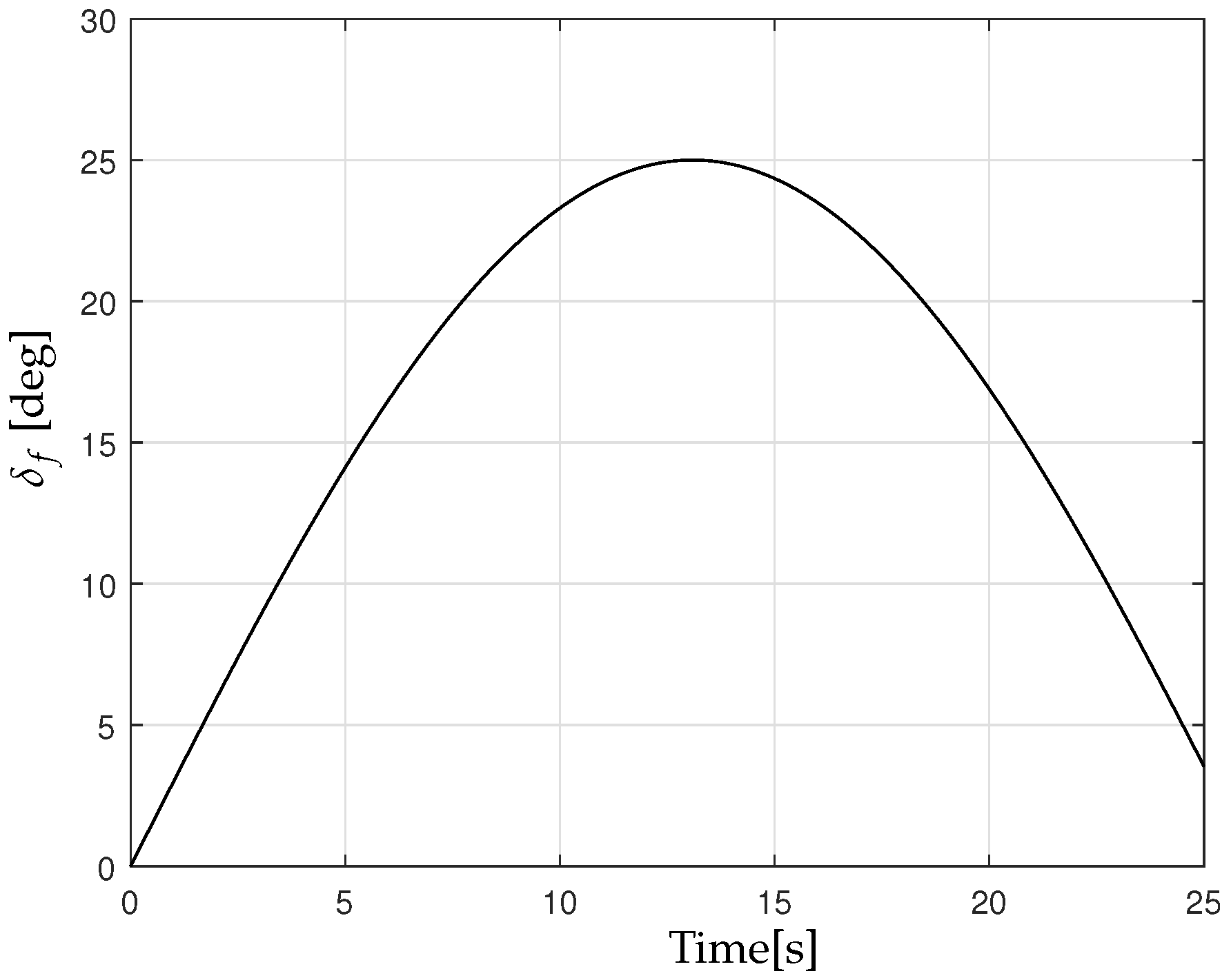
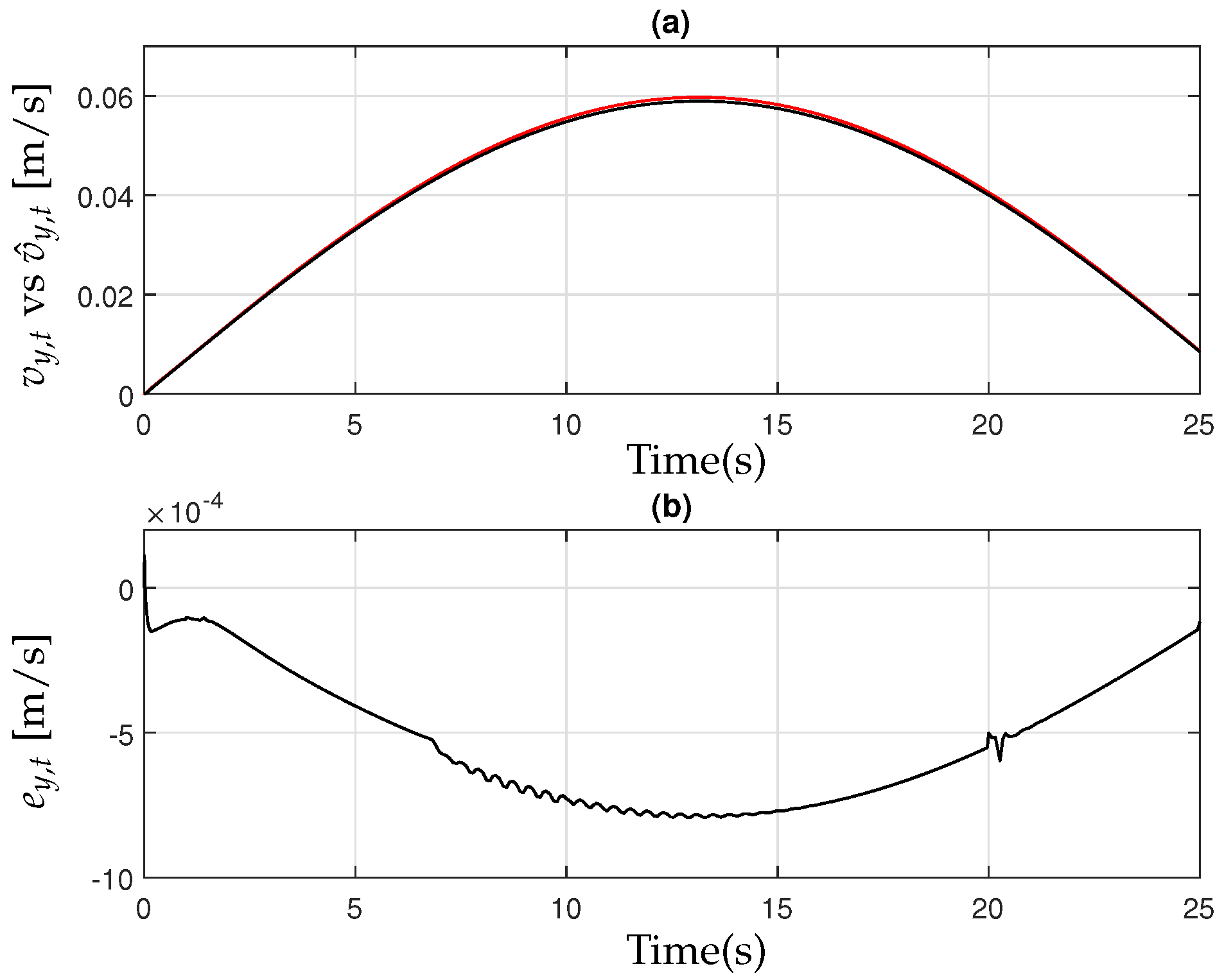
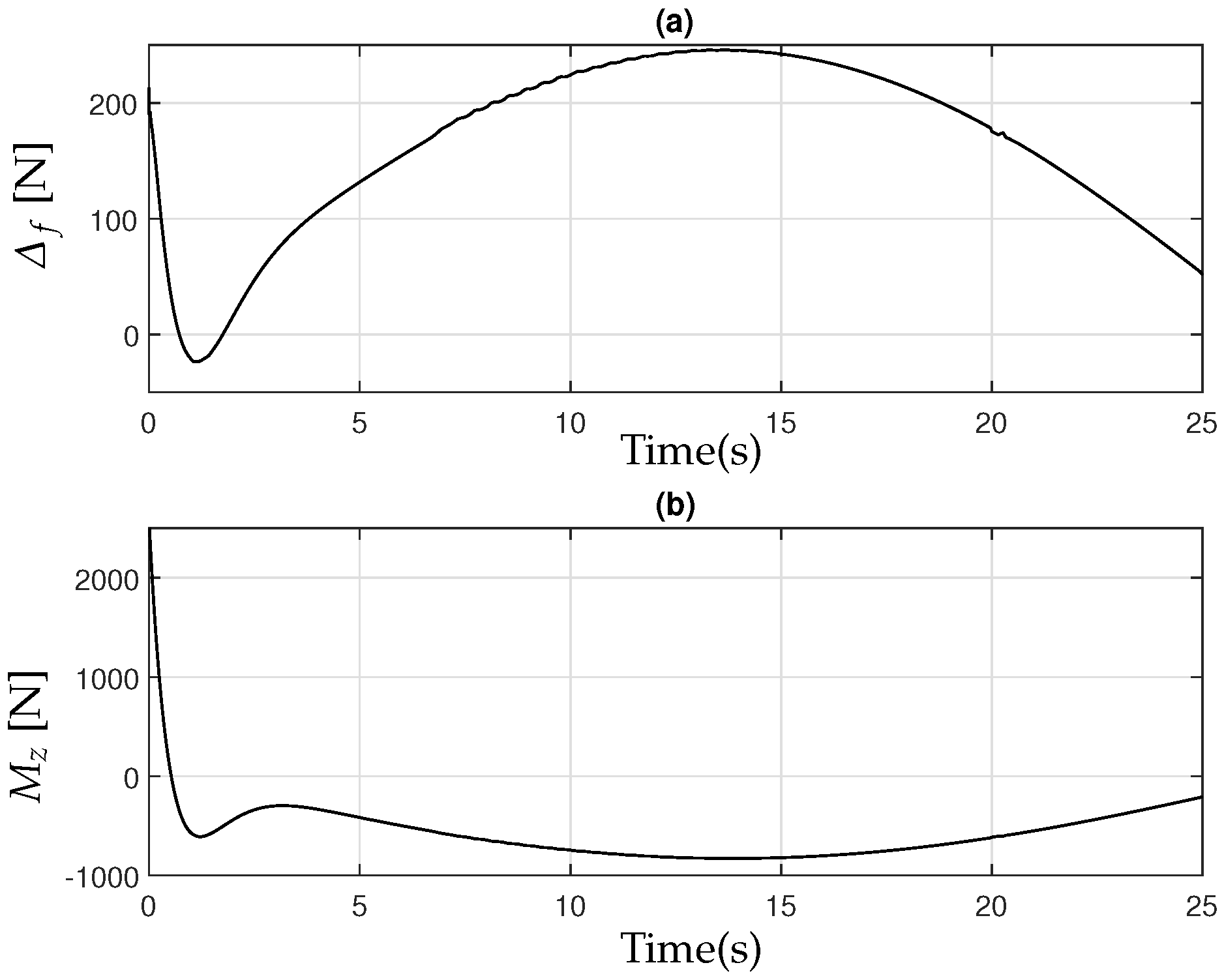
5.1. U-Turn Maneuver

In mechanized agricultural operations, the U-turn or end-of-row turn is a crucial maneuver that enables tractors to change direction at the end of a row and transition seamlessly to the next one. This maneuver is essential for optimizing field coverage and ensuring maximum land utilization. The U-turn maneuver, characterized by a gradual right turn, is analyzed to simulate the tractor’s operational conditions [39,40,41,42]. The dynamic response of the tractor-–implement system defined in (1), under the action of the controller (32), is subsequently assessed. Figure 3 depicts the application of the U-turn maneuver to the steering angle. In standard field operations, farm tractors typically move in straight lines; however, upon reaching the end of a row, they must execute a U-turn to align with the next pass. The direction of the turn, whether left or right, depends on the specific field operation requirements. When towing an implement, a tractor generally completes this maneuver in approximately 25 s, covering an average distance of 15 m.

The results are shown in Figure 4, Figure 5, Figure 6, Figure 7, Figure 8 and Figure 9. The parameters used in the observer (17), and in the controller (32), are shown in

Table 2. Real plant parameter values of (1) and controller gains (32) [35,43].

${\mathit{m}}_{\mathit{t}}=9391$ kg	${\mathit{m}}_{\mathit{i}}=2127$ kg	${\mathit{J}}_{\mathit{z},\mathit{t}}$ = 35,709 kg m2
$J_{z,i}=6402$ kg m2	$l_{f,t}=1.7$ m	$l_{r,t}=1.2$ m
$l_p=2.1$ m	$l_{f,i}=3.62$ m	$l_{r,i}=0.1$ m
$D_{f,t}$ = 36,850.28 N	$C_{f,t}=1.4$ N	$B_{f,t}=4.3$
$D_{r,t}$ = 55,275.38 N	$C_{r,t}=1.5$ N	$B_{r,t}=5.86$
$D_{r,i}$ = 20,865 N	$C_{r,i}=1.5$ N	$B_{r,i}=16$
$k_{o,1}=k_{o,4}=1$	$k_{o,2}=1.8$	$k_{o,3}=1.6$
$k_{1,1}=k_{2,1}=10$	$k_{1,2}=8$	$k_{2,2}=5$

. These values are based on the physical characteristics and system configuration of a JD 7930 tractor and a Parker 500 Grain Cart, as reported in [43] (Ch. 7.2.1., p. 199). “Tractor and towed implement trajectory data was collected on 19 Sepember 2008 in the ISU Agronomy and Agricultural Engineering Research Center (AAERC) located about eight miles west of the ISU central campus. The experimental data was collected using commercially available general purpose GPS receivers (StarFire iTC, Deere and Co., Moline, IL, USA), roll angle compensators, yaw-rate sensors and an integrated wheel angle sensor so that no special instrumentation was required. The field was planted to oats during the prior growing season and was harvested before the tests. A MFWD tractor (model 7930, Deere and Co., Moline, IL, USA) and a single axle 18 m³ (500 bu) grain cart (model 500, Alliance Product Group, Kalida, OH, USA) were used in the experiment”. The JD 7930 is a powerful and versatile tractor designed for heavy-duty agricultural tasks. The JD 7930 is designed for efficiency, comfort, and durability, making it suitable for a wide range of farming operations. Its advanced technology and robust construction ensure high productivity and reliability in demanding conditions. The tractor is equipped with a JD PowerTech Plus engine, which is a 6-cylinder, turbocharged engine. It delivers 175 hp (130.4 kW) at 2100 rpm, with a maximum power of 190 hp (141.7 kW) at 2000 rpm when using Power Management. The John Deere 7930 provides 16 forward and 4 reverse speeds, while the AutoPower is a continuously variable transmission offering infinite speed options. The maximum speed is 40 km/h (25 mph).

Furthermore, the Parker 500 Grain Cart is a high-capacity, durable grain cart designed for efficient harvesting and transport of grain. It is designed for efficiency, durability, and ease of use, making it an excellent choice for farmers who need a reliable solution for transporting large quantities of grain during harvest season. Its robust construction and advanced features ensure high performance and productivity in demanding agricultural environments. The Parker 500 Grain Cart has a total capacity of 500 bushels, making it suitable for large-scale farming operations. The grain tank is constructed from heavy-duty steel, ensuring durability and longevity. The Parker 500 is equipped with heavy-duty axles designed to handle the weight of a full load.

To evaluate the robustness of the controller against parameter uncertainties, the actual plant parameters were set to be 10% higher than the nominal values used in the controller design. This allows the controller to compensate for variations through feedback, reflecting more realistic operating conditions. The values of the specific parameters used in the simulation are summarized in Table 2.

Figure 4 and Figure 5 illustrate the behavior of the observed lateral velocity and yaw rate of the tractor when applying the controller designed in Equation (32) to the tractor–implement system described in Equation (1). Additionally, these figures compare the system’s response with and without control, where the latter scenario represents only the driver’s input without the assistance of the control system. The results demonstrate that the proposed controller effectively tracks the reference trajectories, ensuring stability and minimizing deviations despite the presence of parameter uncertainties. In contrast, when the driver operates the tractor without external control support, the system struggles to follow the given references, leading to increased errors and reduced precision. The lateral velocity closely follows the desired reference with minimal tracking error, enabling smooth and controlled maneuvering during the U-turn operation. Similarly, the yaw rate remains well regulated, preventing excessive oscillations or instability that could compromise the accuracy of the turning process. These findings emphasize the robustness of the proposed control strategy, as it successfully mitigates parameter variations while maintaining stable and reliable performance under dynamic operating conditions.

Then, in Figure 6, Figure 7 and Figure 8, the performance of the observer design presented in Equation (18) can be analyzed in detail. These figures illustrate the estimated states compared to their actual values, demonstrating the accuracy of the observer in reconstructing unmeasured variables such as the lateral velocity, yaw rate, and other critical dynamic parameters of the tractor–implement system. The observer effectively tracks these states with minimal error, ensuring that the estimated values converge rapidly to their true counterparts. This behavior confirms the stability and robustness of the observer under varying operating conditions, including changes in system parameters and external disturbances. The accurate state estimation provided by the observer is crucial for the successful implementation of the integrated active controller, as it allows the system to compensate for uncertainties and enhance overall vehicle stability during field operations.

Finally, the active control inputs ${∆}_f$ due to Active Front Steering (AFS) and $M_z$ due to Rear Torque Vectoring (RTV), obtained in Equation (32), are presented in Figure 9. These inputs play a crucial role in enhancing the stability and maneuverability of the tractor–implement system, particularly during turning maneuvers such as the U-turn. The ${∆}_f$ control input adjusts the front steering angle dynamically, allowing the system to counteract lateral disturbances and maintain the desired trajectory. Simultaneously, the $M_z$ control input generates corrective yaw moments, helping to stabilize the vehicle by distributing torque between the rear wheels. The figure illustrates how these control actions evolve over time, demonstrating their effectiveness in ensuring smooth trajectory tracking and preventing excessive deviations from the reference path. The results confirm that the controller successfully adapts to varying conditions, maintaining stability and optimizing the turning performance of the tractor, even in the presence of parametric uncertainties and external disturbances.

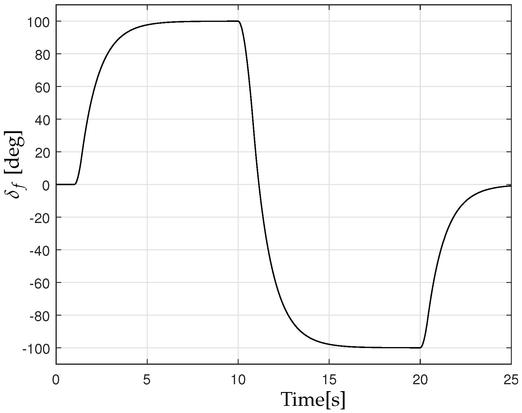
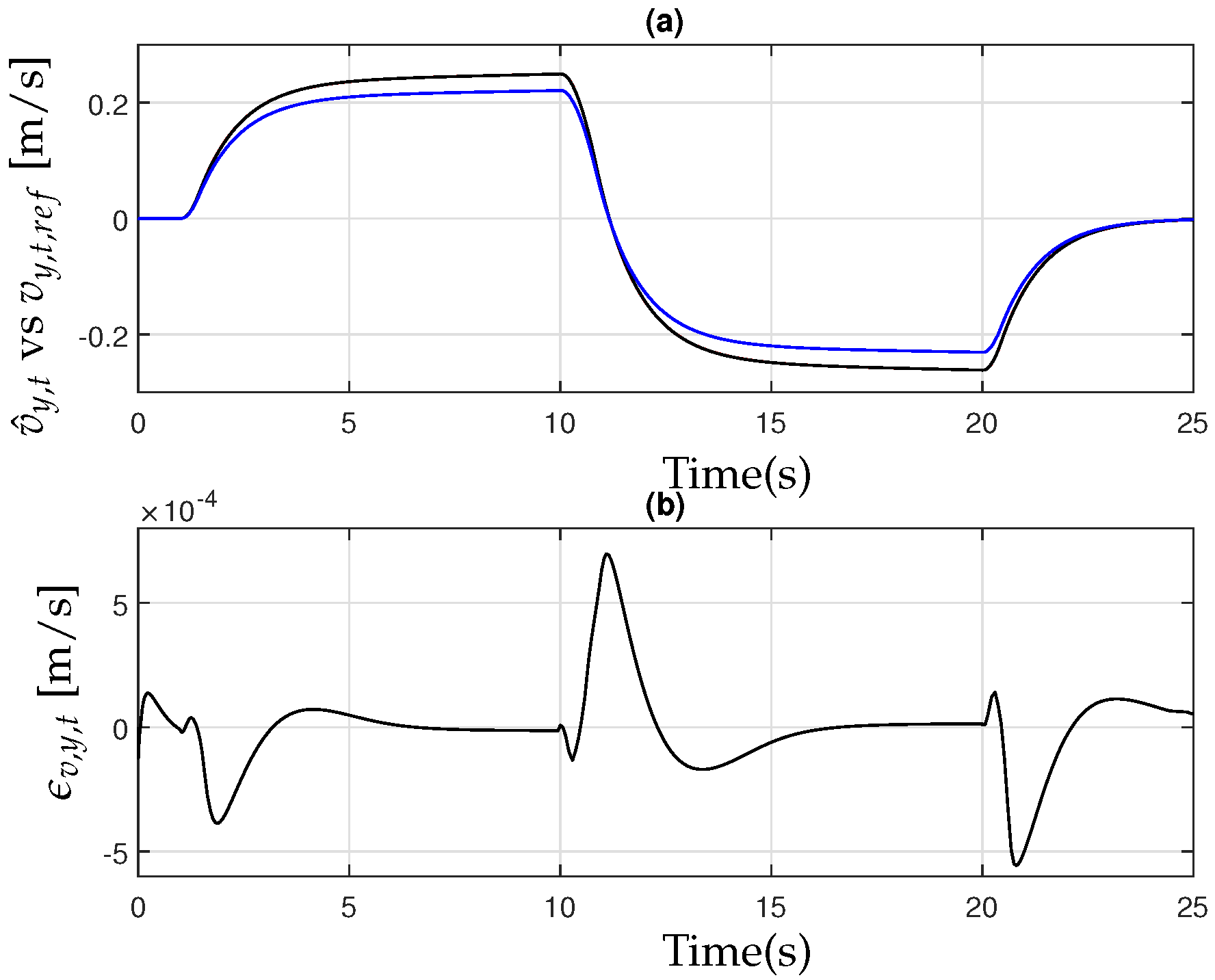
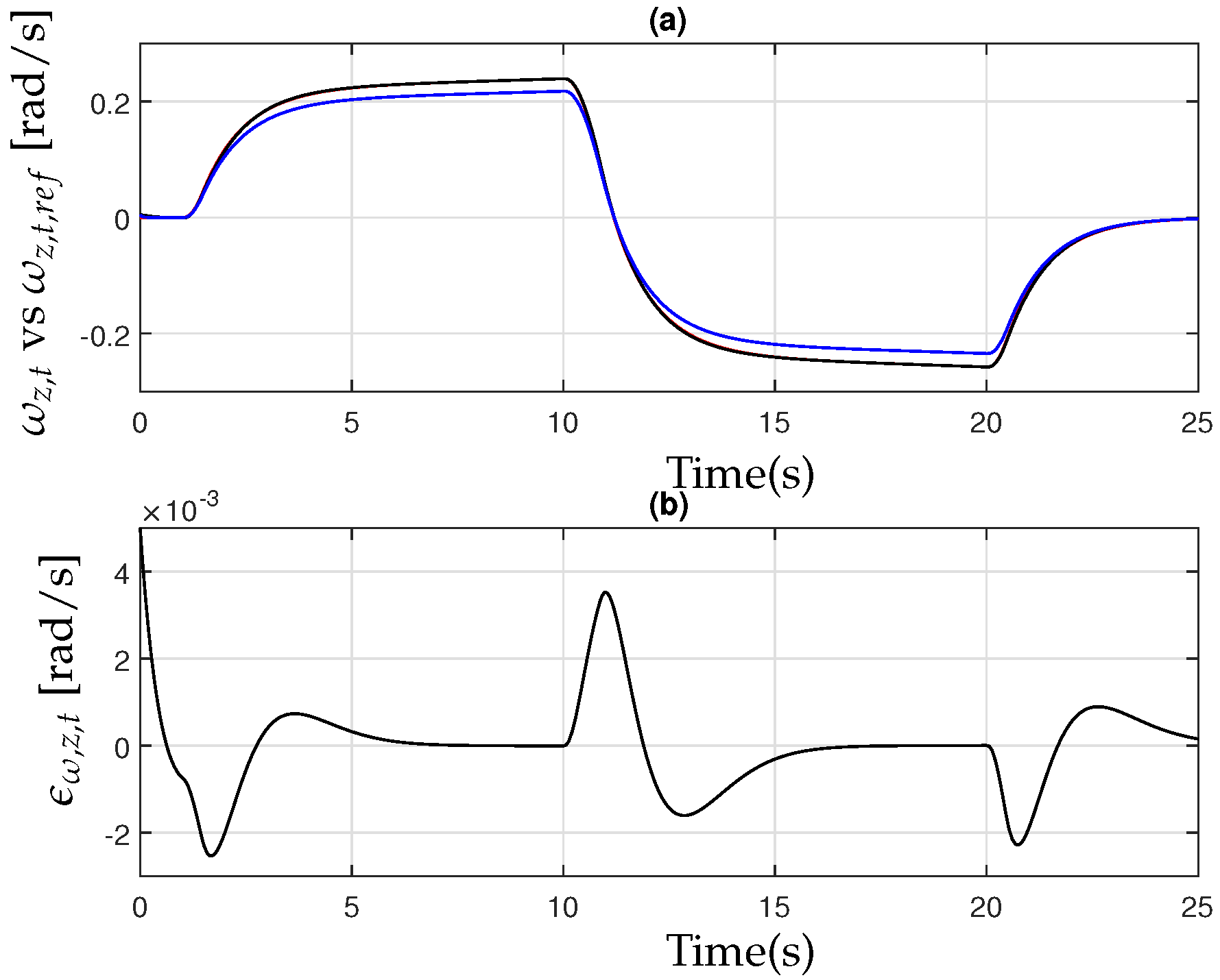
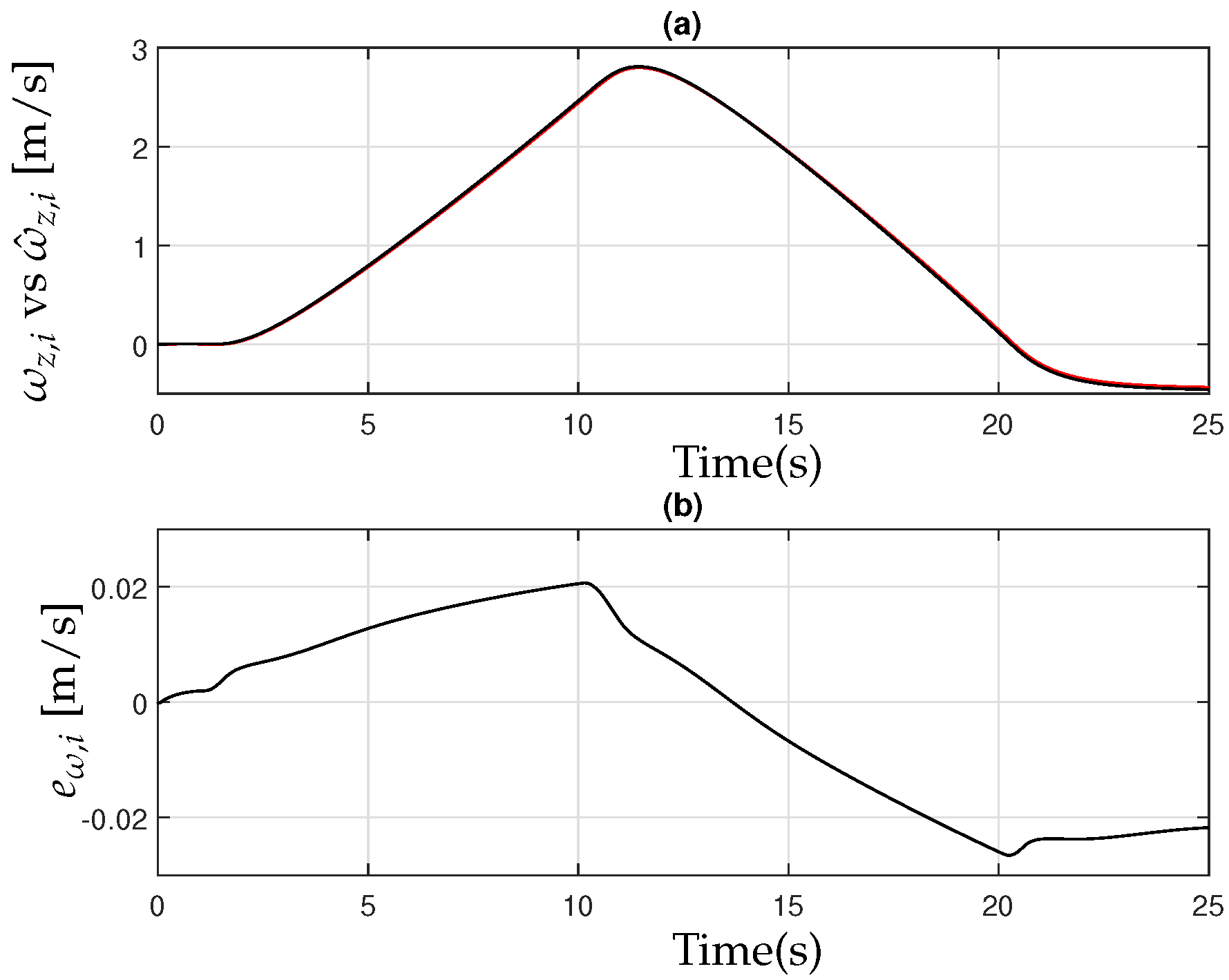
5.2. Double Steer Maneuver

This section presents an alternative demonstration of the robust control performance for the farm tractor with a towed implement under disturbances and parameter uncertainties, as defined in (32). In this case, a more aggressive maneuver, referred to as the double-step maneuver, is employed. This maneuver begins with a sharp left turn of ${100}^{\circ }$ after one second, followed by a rapid right turn of −${100}^{\circ }$ at 10 s. By 20 s, the steering wheel is brought back to its neutral position. Figure 10 provides a visual representation of this maneuver, where a rate limiter is applied to ensure smooth transitions in the steering angle throughout the process [44].

Remark 1. 

The double-step maneuver, commonly used in ground vehicle research, is utilized here to evaluate and confirm the controller’s ability to address the control problem in (20), regardless of the steering input ${\delta }_c$ imposed by the operator.

The parameters applied in both the observer (17) and controller (32) are listed in Table 2.

Figure 11 and Figure 12 illustrate the observed lateral velocity and yaw rate of the tractor when applying the controller designed in (32) to the tractor–implement system described in (1). These results demonstrate the controller’s effectiveness in accurately tracking the reference trajectories, ensuring stability and robustness under varying operating conditions. Additionally, these figures compare the system’s response with and without control, where the latter scenario represents only the driver’s input without the assistance of the control system. The results demonstrate that the proposed controller effectively tracks the reference trajectories, ensuring stability and minimizing deviations despite the presence of parameter uncertainties. In contrast, when the driver operates the tractor without external control support, the system struggles to follow the given references, leading to increased errors and reduced precision. The lateral velocity closely follows the desired reference with minimal tracking error, enabling smooth and controlled maneuvering during the U-turn operation. Similarly, the yaw rate remains well regulated, preventing excessive oscillations or instability that could compromise the accuracy of the turning process. These findings emphasize the robustness of the proposed control strategy, as it successfully mitigates parameter variations while maintaining stable and reliable performance under dynamic operating conditions.

The controller exhibits robust performance even in the presence of parameter uncertainties within the simulation. Figure 13, Figure 14 and Figure 15 further illustrate the effectiveness of the observer design (18), highlighting its ability to accurately estimate system states and maintain stability under varying conditions.

Finally, Figure 16 presents the active control inputs: ${∆}_f$ generated by the AFS and $M_z$ resulting from the RTV, as derived from (32).

6. Conclusions

This paper presented a nonlinear observer-based integrated active control strategy for a farm tractor and its towed implement system. The proposed controller regulates lateral and yaw velocities, ensuring accurate trajectory tracking despite parameter uncertainties. Pacejka’s formula was incorporated to model the nonlinear behavior of tire forces, enhancing the realism of the dynamic response. The proposed control strategy was assessed using Matlab–Simulink simulations, which confirmed its robustness and effectiveness under varying operating conditions. The results confirmed the controller’s capability to maintain stability and performance across standard agricultural maneuvers, including U-turn and double-step tests. The integration of Active Front Steering (AFS) and Rear Torque Vectoring (RTV) further improved the system’s response to external disturbances.

Future work will focus on extending this approach to real-world implementations by conducting experimental validations under different operating conditions. This will involve integrating the proposed observer-based control strategy into a physical tractor–implement system and assessing its performance in field trials. Additionally, we aim to incorporate advanced sensor fusion techniques, such as integrating GNSS, IMU, and vision-based systems, to enhance the accuracy and robustness of state estimation. Another key direction will be the development of adaptive control mechanisms capable of dynamically adjusting to varying terrain conditions, soil properties, and environmental disturbances. Furthermore, we plan to explore real-time implementation challenges, computational efficiency improvements, and potential optimizations to facilitate practical deployment in precision agriculture applications.

References

1. Trimble. Available online: https://ptxtrimble.com/en/products/hardware/guidance-control/nav-500-guidance-controller (accessed on 4 March 2024).
2. John Deere. Future of Farming. Available online: https://www.deere.co.uk/en-gb/your-start-into-the-future-of-farming (accessed on 4 March 2024).
3. Reid, J.; Searcy, S. Vision–based guidance of an agricultural tractor. IEEE Control Syst. Mag. 1987, 7, 39–43. [Google Scholar] [CrossRef]
4. Bell, T. Automatic tractor guidance using carrier–phase differential GPS. Comput. Electron. Agric. 2000, 25, 53–66. [Google Scholar] [CrossRef]
5. Erickson, B.; Widmar, D.A. Precision Agricultural Services Dealership Survey Results; Purdue University: West Lafayette, IN, USA, 2015. [Google Scholar]
6. Poteko, J.; Eder, D.; Noack, P.O. Identifying operation modes of agricultural vehicles based on GNSS measurements. Comput. Electron. Agric. 2021, 185, 106105. [Google Scholar] [CrossRef]
7. Stombaugh, T.S.; Benson, E.R.; Hummel, J.W. Guidance control of agricultural vehicles at high field speeds. Trans. ASAE 1999, 42, 537. [Google Scholar] [CrossRef]
8. Bevly, D.M.; Gerdes, J.C.; Parkinson, B.W. A new yaw dynamic model for improved high-speed control of a farm tractor. J. Dyn. Syst. Meas. Control 2002, 124, 659–667. [Google Scholar] [CrossRef]
9. Bevly, D.M. High Speed, Dead Reckoning, and Towed Implement Control for Automatically Steered Farm Tractors Using GPS. Ph.D. Thesis, Stanford University, Stanford, CA, USA, 2001. [Google Scholar]
10. Pota, H.; Katupitiya, J.; Eaton, R. Simulation of a tractor-implement model under the influence of lateral disturbances. In Proceedings of the IEEE Conference on Decision and Control, New Orleans, LA, USA, 12–14 December 2007; pp. 596–601. [Google Scholar]
11. O’Connor, M.L.; Bell, T.; Elkaim, G.; Parkinson, B. Automatic steering of farm vehicles using GPS. In Proceedings of the Third International Conference on Precision Agriculture, Minneapolis, MN, USA, 23–26 June 1996; pp. 767–777. [Google Scholar]
12. O’Connor, M.L. Carrier–Phase Differential GPS for Automatic Control of Land Vehicles. Ph.D. Thesis, Stanford University, Stanford, CA, USA, 1997. [Google Scholar]
13. Bell, T. Precision Robotic Control of Agricultural Vehicles on Realistic Farm Trajectories. Ph.D. Thesis, Stanford University, Stanford, CA, USA, 1999. [Google Scholar]
14. Eglington, M.; O’Connor, M.; Leckie, L.; Sapilewski, G. System and Method for Guiding an Agricultural Vehicle Through a Recorded Template of Guide Paths. U.S. Patent 20060178820A1, 4 February 2005. [Google Scholar]
15. Blackwell, R.; Schildroth, R.; Myers, M.J.; Rolffs, M.J.; Becker, D. Autonomous Systems, Methods, and Apparatus for Ag-Based Operations. U.S. Patent 20150105963A1, 10 October 2014. [Google Scholar]
16. Basset, D.; Arthur, R.J. Modular Autonomous Farm Vehicle. U.S. Patent 20170164548A1, 11 April 2017. [Google Scholar]
17. Shah, J. Pull–Drift–Compensation Mittels AFS. U.S. Patent 20150105965A1, 3 August 2018. [Google Scholar]
18. Etienne, L.; Acosta Lúa, C.; Di Gennaro, S.; Barbot, J.-P. A Super–Twisting Controller for Active Control of Ground Vehicles with Lateral Tire–Road Friction Estimation and CarSim Validation. IEEE Trans. Control Syst. Technol. 2020, 8, 1177–1189. [Google Scholar] [CrossRef]
19. Acosta Lúa, C.; Di Gennaro, S. Nonlinear adaptive tracking for ground vehicles in the presence of lateral wind disturbances and parameter variations. J. Franklin Inst. 2017, 354, 2742–2768. [Google Scholar] [CrossRef]
20. Acosta Lúa, C.; Castillo–Toledo, B.; Di Gennaro, S. Nonlinear output robust regulation of ground vehicles in presence of disturbances and parameter uncertainties. In Proceedings of the 17th IFAC World Congress, Seoul, Republic of Korea, 6–11 July 2008; pp. 141–146. [Google Scholar]
21. Acosta Lúa, C.; Castillo–Toledo, B.; Cespi, R.; Di Gennaro, S. An integrated active nonlinear controller for wheeled vehicles. J. Franklin Inst. 2015, 352, 4890–4910. [Google Scholar] [CrossRef]
22. Navarrete–Guzmán, A.; Vaca–García, C.C.; Di Gennaro, S.; Acosta Lúa, C. HOSM Controller Using PI Sliding Manifold for an Integrated Active Control for Wheeled Vehicles. Math. Probl. Eng. 2021, 2021, 5482421. [Google Scholar]
23. Grip, H.V.; Imsland, L.; Johansen, T.A.; Fossen, T.I.; Kalkkulhl, J.C.; Suissa, A. Nonlinear vehicle side-slip estimation with friction adaptation. Automatica 2008, 44, 611–622. [Google Scholar] [CrossRef]
24. Zhao, L.H.; Chen, H. Design of a nonlinear observer for vehicle velocity estimation and experiments. IEEE Trans. Control Syst. Technol. 2011, 19, 664–672. [Google Scholar] [CrossRef]
25. Baffet, G.; Stephant, J.; Charara, A. Lateral vehicle–dynamic observers: Simulations and experiments. Int. J. Veh. Auton. Syst. 2007, 5, 184–203. [Google Scholar] [CrossRef]
26. Guo, H.; Chen, H.; Cao, D.; Jin, W. Design of a reduced—Order nonlinear observer for vehicle velocities estimation. IET Control Theory Appl. 2013, 7, 2056–2068. [Google Scholar] [CrossRef]
27. Solmaz, S.; Baçslamiçsli, S. Simultaneous estimation of road friction and sideslip angle based on switched multiple non–linear observers. IET Control Theory Appl. 2011, 6, 2235–2247. [Google Scholar] [CrossRef]
28. Pan, H.; Sun, W.; Gao, H.; Hayat, T.; Alsaadi, F. Nonlinear tracking control based on extended state observer for vehicle active suspensions with performance constraints. Mechatronics 2014, 30, 363–370. [Google Scholar] [CrossRef]
29. Shen, X.; Liu, G.; Liu, J.; Gao, Y.; Leon, J.I.; Wu, L.; Franquelo, L.G. Fixed-time sliding mode control for NPC converters with improved disturbance rejection performance. IEEE Trans. Ind. Inform. 2025. [Google Scholar] [CrossRef]
30. Vo, A.T.; Truong, T.N.; Le, Q.D.; Kang, H.-J. Fixed-Time Sliding Mode-Based Active Disturbance Rejection Tracking Control Method for Robot Manipulators. Machines 2023, 11, 140. [Google Scholar] [CrossRef]
31. Giap, N.V.; Vu, H.S.; Nguyen, Q.D.; Huang, S.C. Disturbance and Uncertainty Rejection-Based on Fixed-Time Sliding-Mode Control for the Secure Communication of Chaotic Systems. IEEE Access 2021, 9, 133663–133685. [Google Scholar] [CrossRef]
32. Shen, X.; Liu, J.; Liu, G.; Zhang, J.; Leon, J.I.; Wu, L.; Franquelo, L.G. Finite-time sliding mode control for NPC converters with enhanced disturbance compensation. IEEE Trans. Circuits Syst. Regul. Pap. 2024, 72, 1822–1831. [Google Scholar] [CrossRef]
33. Meng, J.; Tan, H.; Jiang, L.; Qian, C.; Xiao, H.; Hu, Z.; Li, G. Robust Finite-Time Sliding Mode Control of Unmanned Surface Vehicle with Active Compensation of Pose Estimation Uncertainty. Ocean Eng. 2024, 304, 117831. [Google Scholar] [CrossRef]
34. Shen, X.; Liu, J.; Liu, Z.; Gao, Y.; Leon, J.I.; Vazquez, S.; Wu, L.; Franquelo, L.G. Sliding mode control of neutral-point-clamped power converters with gain adaptation. IEEE Trans. Power Electron. 2024, 39, 9189–9201. [Google Scholar] [CrossRef]
35. Karkee, M.; Steward, B.L. Study of the open and closed loop characteristics of a tractor and a single axle towed implement system. J. Terramech. 2010, 47, 379–393. [Google Scholar] [CrossRef]
36. Pacejka, H. Tyre and Vehicle Dynamics; Elsevier Butterworth–Heinemann: Butterworth, Malaysia, 2005. [Google Scholar]
37. Imsland, L.; Johansen, T.A.; Fossen, T.I.; Grip, H.V.; Kalkkulhl, J.C.; Suissa, A. Vehicle estimation using nonlinear observer. Automatica 2006, 42, 2091–2103. [Google Scholar] [CrossRef]
38. Khalil, H.K. Nonlinear Systems; Prentice–Hall: Englewood Cliffs, NJ, USA, 2002. [Google Scholar]
39. Lee, M.F.R.; Nugroho, A.; Purbowaskito, W.; Bastida, S.N. Path Following for Autonomous Tractor under Various Soil Conditions and Unstable Lateral Dynamic. In Proceedings of the 2020 International Conference on Advanced Robotics and Intelligent Systems (ARIS), Taipei, Taiwan, 19–21 August 2020; pp. 1–6. [Google Scholar] [CrossRef]
40. Lei, G.; Zhou, S.; Zhang, P.; Xie, F.; Gao, Z.; Shuang, L.; Xue, Y.; Fan, E.; Xin, Z. Stability Control of the Agricultural Tractor-Trailer System in Saline Alkali Land: A Collaborative Trajectory Planning Approach. Agriculture 2025, 15, 100. [Google Scholar] [CrossRef]
41. Cutini, M.; Bisaglia, C.; Brambilla, M.; Bragaglio, A.; Pallottino, F.; Assirelli, A.; Romano, E.; Montaghi, A.; Leo, E.; Pezzola, M.; et al. A Co-Simulation Virtual Reality Machinery Simulator for Advanced Precision Agriculture Applications. Agriculture 2023, 13, 1603. [Google Scholar] [CrossRef]
42. Qu, J.; Zhang, Z.; Qin, Z.; Guo, K.; Li, D. Applications of Autonomous Navigation Technologies for Unmanned Agricultural Tractors: A Review. Machines 2024, 12, 218. [Google Scholar] [CrossRef]
43. Karkee, M. Modeling, Identification and Analysis of Tractor and Single Axle Towed Implement System. Ph.D. Dissertation, Iowa State University, Ames, IA, USA, 2008. [Google Scholar]
44. Wang, H.; Noguchi, N. Real-time states estimation of a farm tractor using dynamic mode decomposition. GPS Solut. 2021, 25, 16. [Google Scholar] [CrossRef]
Figure 1. Schematic of the tractor–implement dynamics.
Electronics 14 01575 g001
Figure 2. Forces acting on the tractor–implement system.
Electronics 14 01575 g002
Figure 3. Steering angle δ d .
Electronics 14 01575 g003
Figure 4. (a) Closed−loop representation of the estimated lateral velocity of the agricultural tractor, v ^ y , t , and its reference, v y , t , r e f [red], comparing the response with the nonlinear control (32) [black] and without it (32) [blue]; (b) tracking error ϵ v , y , t .
Electronics 14 01575 g004
Figure 5. (a) Closed−loop representation of the farm tractor’s yaw rate, ω z , t , alongside its reference value, ω z , t , r e f [red], comparing the response with the nonlinear control (32) [black] and without it (32) [blue]; (b) tracking error, ϵ ω , z , t .
Electronics 14 01575 g005
Figure 6. (a) Longitudinal velocity of the farm tractor v x , t [black] and observer v ^ x , t [red]; (b) the observer error e x , t .
Electronics 14 01575 g006
Figure 7. (a) Farm tractor’s lateral velocity v y , t [black] and observer v ^ y , t [red]; (b) the observer error e y , t .
Electronics 14 01575 g007
Figure 8. (a) Yaw rate of the implement ω z , i [black] and observer ω ^ z , i [red]; (b) the observer error e ω , i .
Electronics 14 01575 g008
Figure 9. (a) Active Front Steering in closed-loop representation: f control; (b) Rear Torque Vectoring, M z control.
Electronics 14 01575 g009
Figure 10. Steering angle δ d .
Electronics 14 01575 g010
Figure 11. (a) Closed-loop representation of the estimated lateral velocity of the agricultural tractor, v ^ y , t , and its reference, v y , t , r e f [red], comparing the response with the nonlinear control (32) [black] and without it (32) [blue]; (b) tracking error ϵ v , y , t .
Electronics 14 01575 g011
Figure 12. (a) Closed-loop representation of the farm tractor’s yaw rate, ω z , t , alongside its reference value, ω z , t , r e f [red], comparing the response with the nonlinear control (32) [black] and without it (32) [blue]; (b) tracking error, ϵ ω , z , t .
Electronics 14 01575 g012
Figure 13. (a) Longitudinal velocity of the farm tractor v x , t [black] and observer v ^ x , t [red]; (b) the observer error e x , t .
Electronics 14 01575 g013
Figure 14. (a) Lateral velocity of the farm tractor v y , t [black] and observer v ^ y , t [red]; (b) the observer error e y , t .
Electronics 14 01575 g014
Figure 15. (a) Yaw rate of the implement ω z , i [black] and observer ω ^ z , i [red]; (b) the observer error e ω , i .
Electronics 14 01575 g015
Figure 16. (a) Active Front Steering in closed-loop representation: f control; (b) Rear Torque Vectoring, M z control.
Electronics 14 01575 g016