Abstract
The control of vehicles towing trailers is of significant interest to industry due to their wide-ranging applications across various sectors. Trailers play essential roles in logistics, mining, and other fields. This study focuses on the control of a dumper with a trailer specifically used for the monitoring of terrain stability in mining operations. The trailer is equipped with a radar system for detecting potential ground shifts that could jeopardize fieldwork safety. While numerous studies have addressed the control of Ackerman vehicles and trailers, this dumper presents a unique challenge due to its rear-axle steering mechanism. Due to this configuration, which has not been extensively studied in the literature, although the differential flatness of the system is proven, computation of the flat outputs leads to a system of partial differential equations that cannot be solved analytically. For this reason, this paper examines partial feedback linearization to facilitate control and proposes a solution for trajectory tracking that also stabilizes jack-knifing tendencies between the vehicle and trailer. The designed control system was successfully validated in a virtual environment.
1. Introduction
Interest in controlling vehicles with trailers is significant due to their crucial role in industry. These areas encompass logistics in factories, road transportation, and agricultural activities such as tractor–trailer combinations. The trajectory tracking problem for vehicles with trailers is more complex due to the inherent non-linearity of the system, the kinematic characteristics of the tractor vehicle, and constraints on actuation margins (e.g., maximum/minimum steering angles and steering speed limits). Furthermore, the system’s behavior varies based on the steering direction, which can lead to potential loss of controllability. Additionally, perturbations like sliding, slack between elements, or friction may also affect the system’s dynamics. Previous research has explored control strategies for these systems from diverse perspectives. It is worth mentioning the solutions described by Rouchon et al. [1], namely an Ackerman tractor vehicle system with a series of passive trailers that was proven to be linearizable by applying differential flatness when the rotation point between consecutive elements was placed on the rear axle of every vehicle. This condition is no longer valid when there is more than one trailer and the rotation point is not located on the axle [2]. For some particular cases, for example, a tractor vehicle with an active trailer, it is, again, possible to linearize the system by means of flatness, then to exploit this property for trajectory planning and control [3]. In other cases, it is common to apply partial linearization of the system, as in the work by Altafini et al. [4]. A different controller is selected in their proposal depending on the type of movement (forwards; backwards, following a straight line; and a curve), and it is obtained by linearizing the system along the trajectory and applying LQ (Linear Quadratic) optimal control in every mode. A similar procedure was described in the work by Evestedt et al. [5]. Werling et al. [6] sought a general stabilization procedure for any possible relative angular movement between a tractor vehicle and trailer by applying input–output linearizations. Afterwards, it was incorporated in the global vehicle–trailer controller by linearizing the whole system along the trajectory. Previous examples have considered the slip between the wheel and the terrain to be negligible. In order to solve the case considering slip, Alipour et al. included this effect through the LuGre friction model and applied sliding control to compensate for perturbations derived from it [7]. The slip effect was also studied in the case of a tractor vehicle with an active trailer, where the movement was stabilized by combining backstepping techniques for the motion of the tractor and a non-linear PI (Proportional Integral) controller for the trailer angle [8].
The theory of differential flatness has been successfully applied in the past to control a wide range of industrial applications. The method has proven its robustness in different systems, and the coupling between the trajectory and the controller that arises from the differential flatness property makes it specially useful for trajectory tracking applications. The following application examples show the widespread possibilities of flatness for the design of robust controllers: autonomous robots for logistics control in [9]; components of the automotive industry like [10] for motors in electric vehicles or [11] for synchronized movement of windshield wipers, construction machinery like [12,13] for the position control of loads on tower cranes, and energy-sector applications like [14] for the control of gas-turbine power generation. One of its key advantages is that it provides a powerful tool for developing control algorithms, particularly for linear and non-linear systems. A system with differential flatness exhibits a unique property: its reference trajectory can be uniquely defined through a diffeomorphism with the control law. This relationship enables the incorporation of differential flatness into feedforward control schemes, providing a robust foundation for control design. By augmenting this feedforward approach with a feedback loop that refines the control action, improved performance can be achieved. The application of differential flatness has been particularly successful in solving the driftless navigation problem for vehicles with and without trailers, where it has enabled efficient and stable control [2,15]. In recent years, these results have been extended towards scenarios with drifting wheels and higher velocities, both in the controller (longitudinal and lateral control), and in the local planner [16]. In this case, the simplicity of calculations is exploited for real-time applications.
In the development of autonomous vehicles, the coupling between the navigation system and the low-level controllers is significant. In this connection, the local planner is especially important, as it is responsible for defining the trajectory of the vehicle and doing so in accordance with the vehicle characteristics and environmental conditions (road shape, obstacles, etc.). This local planner is sometimes directly linked with the longitudinal and lateral controllers, but some architectures separate the two approaches, thereby simplifying the optimization process. A possible approach in this connection is the use of differential flatness [15], which permits the definition of a feasible trajectory, keeping the kinematic restrictions and obtaining a feedforward command in a straightforward way. This is also the approach used by Volvo trucks [17]. The trajectory can be optimized using receding horizon optimizations like MPC (Model Predictive Control) or others. The consideration in this local planner optimization of all restrictions and data coming from system estimators (road traction limits, side angle, slope and bank angle, etc.) permits a reduction in the complexity of the low-level controllers (for example, by using MPC [18]). It is worth mentioning that no previous study has dealt with the control of a rear-axle steering vehicle connected to a trailer.
Another challenge that must be tackled to control vehicles with trailers is the jack-knifing effect. This behavior may appear when performing certain driving maneuvers or under slippery road conditions, and it causes a folding between the vehicle and the trailer. Such undesired folding affects the control strategy to the extent that it can make it unstable. Compared to other strategies for compensating for jack-knifing, the proposed approach uses a different controller once the vehicle reaches difficult conditions, which is similar to what a human driver would do. The proposed approach combines trajectory tracking focused on the front vehicle with a relative angle compensator that only operates in case of jack-knifing. This strategy differs from other approaches in the literature. For example, Ref. [6] used a linearization technique around the operation point to calculate the maximum affordable curvature of the trajectory and modify the followed path accordingly. Ref. [4] linearized the system for straight and curved trajectories and calculated a linear controller that stabilizes the system, including the angles of the vehicle and trailer, along those tracks. Similarly, in [19], the vehicle used a two-level controller, as well as a pure pursuit trajectory tracker at the highest level, combined with an orientation controller at the lower level. The latter control loop avoids risky conditions by using a stabilizing controller to reach the look-ahead reference orientation. These strategies limit the relative angle all along the trajectory, considerably reducing the admitted maneuvers. In the proposed strategy, which also uses linearization techniques, the relative angle compensator only actuates when a certain threshold has been exceeded and tries to perfectly track the desired trajectory until that moment, even if the relative angle considerably increases. This is so because the vehicle operates at a low speed and the scanning application needs higher versatility in terms of the admitted maneuvers and derived angles in order to adapt the movement to the terrain restrictions.
The current work is focused on the trajectory tracking of a rear-axle steering dumper connected to a trailer. To the best of the knowledge of the authors, this use case has not been studied in the literature, showing important challenges in terms of control. The main contributions of the paper are a mathematical analysis of the problem, partial feedback linearization of the system, and application to the design of a trajectory tracking controller. During the analysis, the proof of the differential flatness of the system is given, which opens the possibility of applying some successful controllers for vehicles with trailers, and the further derivation of a proper controller. However, computation of the flat outputs leads to a system of partial differential equations that cannot be solved analytically. To overcome this issue, partial state feedback combined with a compensator for avoiding jack-knifing is proposed and successfully validated under virtual conditions. The algorithm for partial feedback linearization of control systems was outlined in [20], and it has been successfully implemented in other mechanical systems, as in [21], where a controller for a Segway was designed.
This paper is organized in six sections. After the Introduction, the problem is described in Section 2. The mathematical analysis of the system and the potential linearizations appear in Section 3. A possible controller based on this linearization is proposed in Section 4 and tested under simulated conditions in Section 5. The conclusions appear in Section 6.
2. Problem Statement
2.1. Description
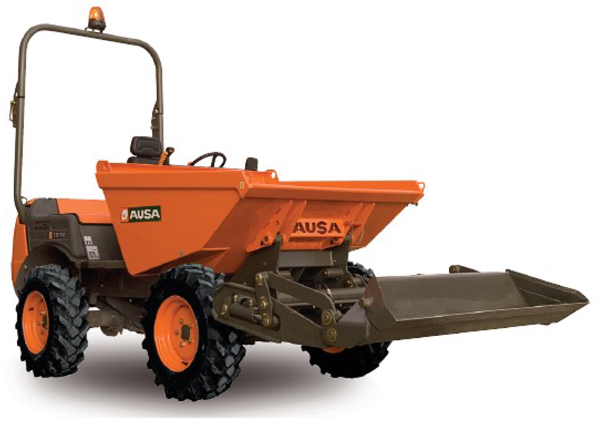
The present work is part of a larger project to continuously monitor the status of a mine (see funding information at the end of the paper for the details of the project). Continuous earth movement often leads to the formation of unstable ground areas. To address this, the project proposes the combined use of autonomous vehicles and drones with sensors for the monitoring of changes in the carved working face of the mine. The present paper focuses on the control problem of autonomous vehicles equipped with radar sensors on trailers. The vehicles are dumpers with hydraulic traction and steering systems (Figure 1). A unique aspect is that the steering wheels are located at the rear axle, which, as explained in the next section, has a significant impact on the controllability of the combined vehicle and trailer.

Figure 1.
Dumper vehicle studied in the present work and used in the real mining environment.
The main dimensions of the system vehicle and trailer are summarized in Table 1.

Table 1.
Main dimensions of the vehicle and trailer.
2.2. Setup Approach
With the purpose of implementing the control system, the dumper in Figure 1 was equipped with different sensors and processing units. We obtained the velocities of the dumper and the trailer by combining data from Ardusimple GPS (Global Positioning System) devices with two antennas, IMUs (Inertial Measurement Units), and Hall-effect wheel encoders. The absolute orientation of the dumper was obtained from the GPS, and the relative angle between the dumper and the trailer was determined by processing the point cloud obtained by a Sick TIM-571 laser (Sick, Germany) installed on the rear part of the dumper. In addition, the surrounding environment was detected thanks to an Ouster OS-1-128 LIDAR (Ouster, USA) instrument mounted at the top of the vehicle, two Livox HAP (Livoxtech, China) modules installed on the front and rear parts, two HESAI FT120 LIDARs (Hesai, China) located on the right and left sides, and two industrial-degree Blackfly POE RGB cameras (Teledyne, USA) positioned on the top-front and top-rear sides. All sensors were connected to an onboard PC to reduce communication delays, including an Intel Core i9 5GHz 16-core processor (Intel, USA).
This combination of devices allowed us to minimize the real-world uncertainties that cannot be represented in the virtual validation environment.
3. Differential Flatness and Partial Feedback Linearization
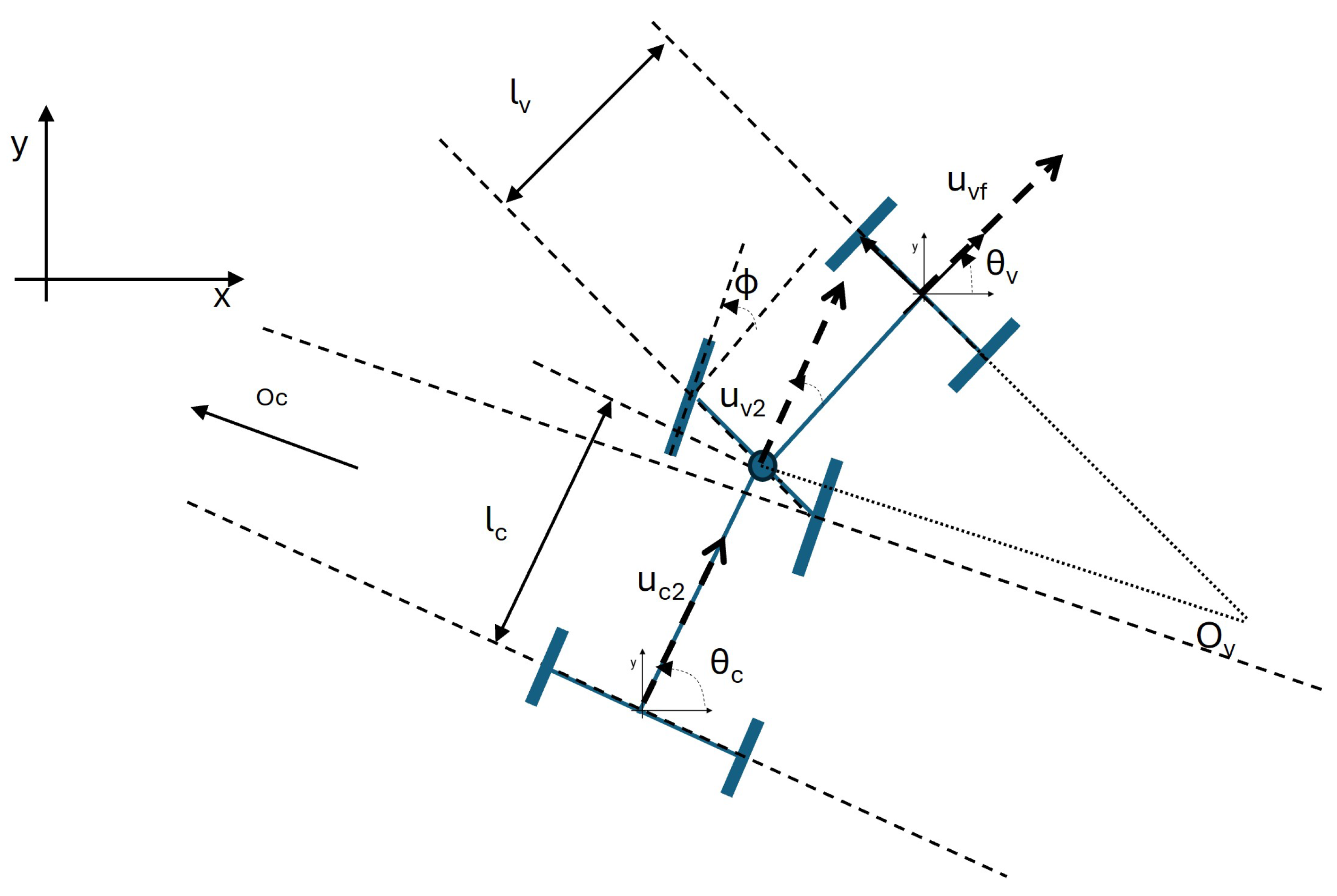
Due to the low speeds and the load of the vehicle and trailer, the dynamics of the system are represented under non-sliding conditions. A schema with the main variables of the system is presented in Figure 2.
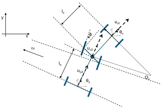
Figure 2.
Schematic of the vehicle showing the main parameters involved. and are the instantaneous centers of rotation for the vehicle and the trailer, respectively (the arrows show the positive sense of the angle).
Although it is possible to represent the system in different ways depending on the axle at which the reference is placed, we study a case with the reference in the vehicle’s front axle. As the speed on the front axle () is the longitudinal control action, it makes sense to describe the movement from that reference. The lateral control action is the steering-wheel angle (). The resulting evolution of the front axle’s center position (, ) and the orientation of the vehicle () and trailer () can be described as follows:
In order to simplify the notation, we will denote
The system is not in affine form. Hence, a new state () is added with the corresponding additional equation (), obtaining a two-input driftless system:
The vector fields associated with this system are
and the necessary and sufficient condition for flatness given by Martin and Rouchon in [22] can be checked by computing the following distributions:
It is a straightforward computation to check that the dimension of is , ∀. According to [22], this implies the flatness of the system. However, the authors were not able to find the flat outputs of (2) by applying the algorithms given in [22] because this led to a system of partial differential equations that cannot be solved analytically. Similarly, the application of the results presented in [23,24] also faces this issue.
On the other hand, the system is not linearizable by pure prolongations ([25,26]); therefore, flat outputs cannot be computed using this method either.
An alternative method to control the system is to partially feedback linearize the representation. In order to do this, we use the construction given in [20]. Consider the following sets and distributions:
where f is the drift vector field, while and are the input vector fields, , , represents the involutive closure of , , and . Based on the former definitions, we compute the following integers:
Then, it follows that and the maximum relative degree that one can achieve for a given system is .
Before computing all these distributions and integers for and as given in (2), we apply a prolongation of the system; otherwise, , and the algorithm is not useful. More precisely, a two-order prolongation of input is performed, resulting in the following overall system:
Applying the above mentioned algorithm, distributions and are both involutive and of dimensions 2 and 4, respectively. On the other hand, , , and are of dimensions 2, 4, and 6 respectively. Therefore,
and . Therefore, the dimension of the maximum linearizable subsystem is . Finally, the dimensions of each of the Brunovsky boxes of the linearizable part are
In order to find the change of variables that partially linearize the system, two functions ( and ) must be found. These functions must fulfill the property that their relative degrees are and , and they must be differentially independent—in other words, the Jacobian of must not be singular.
It is not difficult to check that and do the job. Therefore, the change of variables to partially feedback linearize the system is expressed as follows:
The seventh variable of the change of variable can be chosen freely as long as it is differentially independent with . For instance, is a simple choice.
Regarding the feedback, the new inputs are defined in such a way that, in the new variables, the system is in Brunovsky form for the first six variables. Hence, and . Therefore, the feedback law is expressed as follows:
After applying the change of variables and the feedback law, the equations of the system become the following:
The seventh equation is obtained by computing
which, after application of the inverse of the diffeomorphism in order to write all the x variables as functions of the z variables and some bookkeeping, reads
The transformation from to changes depending on the speed direction:
- For a positive speed,
- For a negative speed,
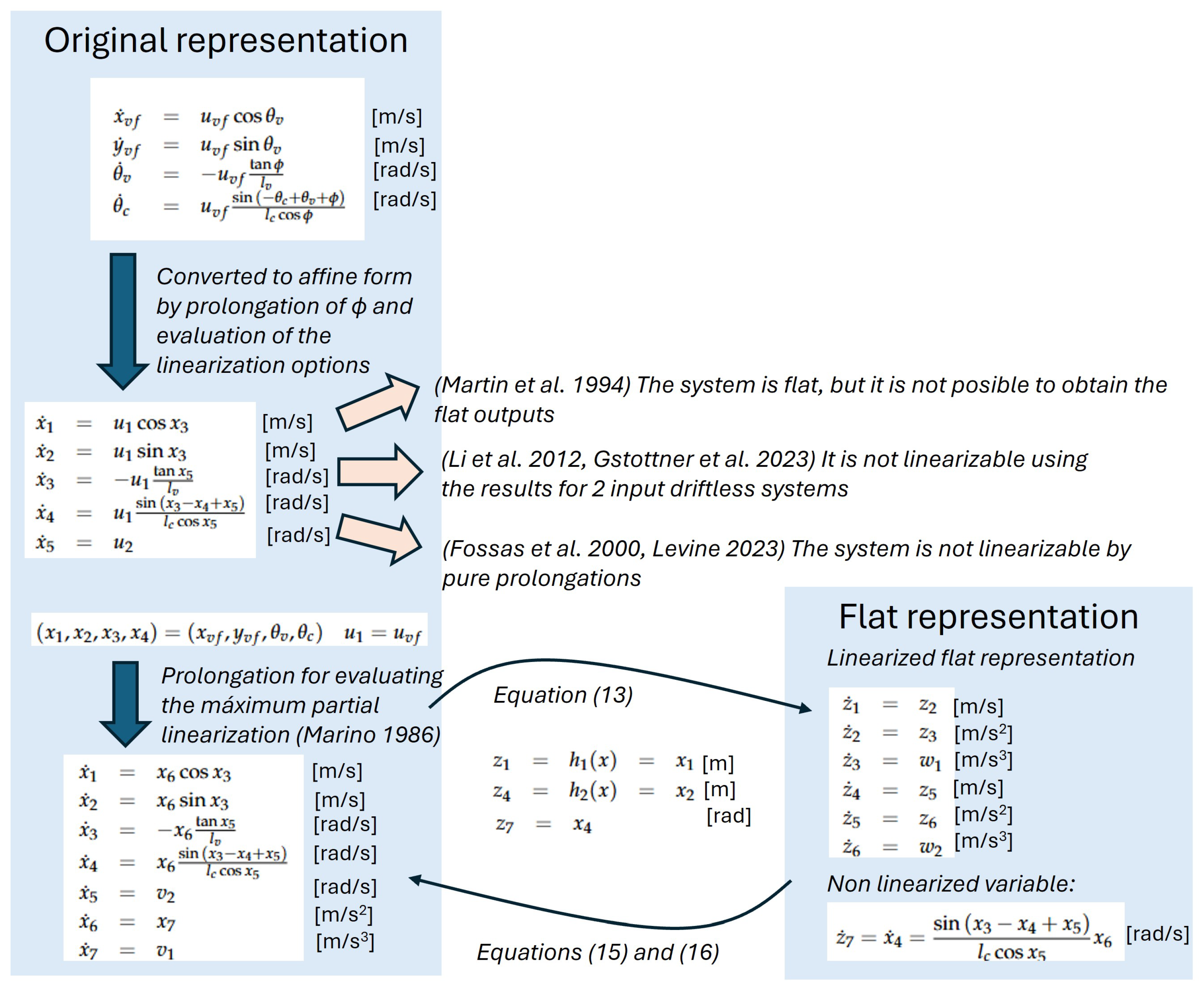
Figure 3 summarizes the followed process for linearizing the systems and the transformation between the original and the linear representation.
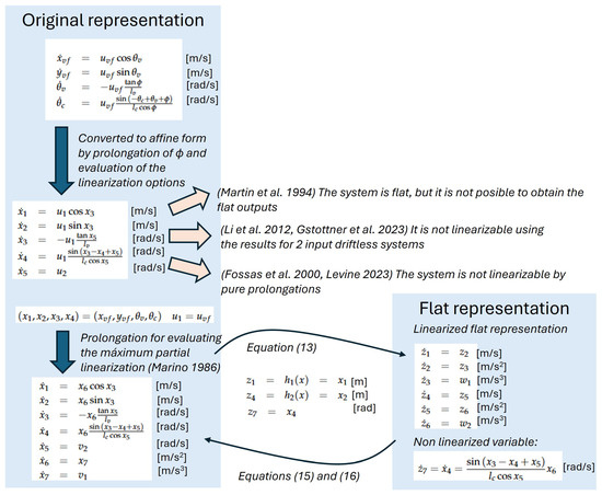
Figure 3.
Summary of the linearization process and the change of variables. The evaluation of the differential flatness is done according to Martin et al. 1994 [22]. The obtainment of the flat outputs is first evaluated by using the results from Li et al. 2012 [23] and Gstottner et al. 2023 [24] for 2 input driftless systems, and the results from Fossas et al. 2000 [25] and Levine 2023 [26] by using prolongations. None of these approaches worked, and it is finally decided to solve the problem by using the partial linearization described in Marino 1986 [20].
4. Control Design
The control structure is shown in Figure 4, where the same non-slippery condition considered in the previous sections is assumed. The trajectory is generated in the linearized representation corresponding to and and their derivatives. The figure also shows where the diffeomorphism between the x and z variables is applied. This approach is convenient because both variables correspond to the desired geometrical path, speed, acceleration, and jerk. After that, the control action can be computed in two different ways depending on the relative angle between the vehicle and the trailer. In case this angle exceeds a certain threshold, the trajectory tracking mode switches to relative angle compensation to avoid jack-knifing.
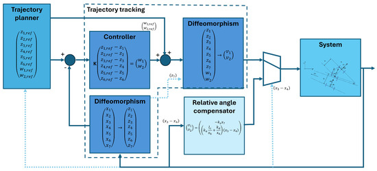
Figure 4.
Description of the control loop.
The trajectory tracking control is given in the linearized space as described in the previous section, and the obtained action is transformed into the original system input by using the diffeomorphism ((15) and (16)). The command has two terms: a feedforward action directly obtained from the theoretical trajectory and a state space feedback in (vector variables are remarked using bold font). The latter is calculated by using (14):
The state feedback command () is obtained as follows:
where . is calculated to fix the poles of the closed-loop system, as described by the error dynamics below:
The trajectory tracking controller in Figure 4 is complemented by the relative angle compensator, which takes control of the steering when the angle between the vehicle and trailer approaches a jack-knife condition. Jack-knifing can produce a risky situation that would damage both the vehicle and the radar on the trailer. To avoid that, when rad, () keeps the speed by setting as a reference, and () reduces the relative angle between vehicle and cart (). A threshold of 1.3 rad is chosen because it allows for a relative angle, which may be necessary to place the vehicle in a correct position for certain measurements of the radar system, although it avoids largely exceeding rad. This threshold can be modified depending on the application and vehicle characteristics. When compensation is activated, the speed control changes to the following:
This way, the acceleration of the vehicle is set to zero in order to keep a constant speed (). The value of is chosen according to the desired response time () of the system to keep a constant speed:
The lateral action () is defined as follows:
, , and are positive control gains. s is the Laplace transform of the derivative. The shape of the controller is decided to obtain a sort of proportional-integral compensator in the relative angle , as described in the following. The division by compensates for part of the speed dependence in the error dynamics.
Using and in (10) at a constant speed of and small angles of , the dynamics of the relative angle are described as follows:
The above equation shows that the system tends to increase the relative angle between the trailer and vehicle () once a small movement of the steering wheel is applied (). The equation below shows that the relative angle tends to increase and the system is unstable in backward movements presenting a positive pole in the linearized first-order system below, obtained by a linearization assuming a small relative angle:
For the relative angle controller, the system is linearized using first-order Taylor approximation at the following operation points: and . The result in the first operation point is:
As , its derivative becomes the following:
This result is used to substitute (22) in (25). The obtained error equation after applying the Laplace transform becomes the following:
where and . The term on the right is a consequence of using . In consequence, when the vehicle and trailer approach a risky situation, the compensator tries to align them by sending a command.
To ensure stability at all speeds, it suffices to impose the following condition:
The value of is fixed to define the response time of the relative angle controller. A summary of the gain calculation appears in Table 2.
Table 2.
Sizing procedure for the relative angle compensator.
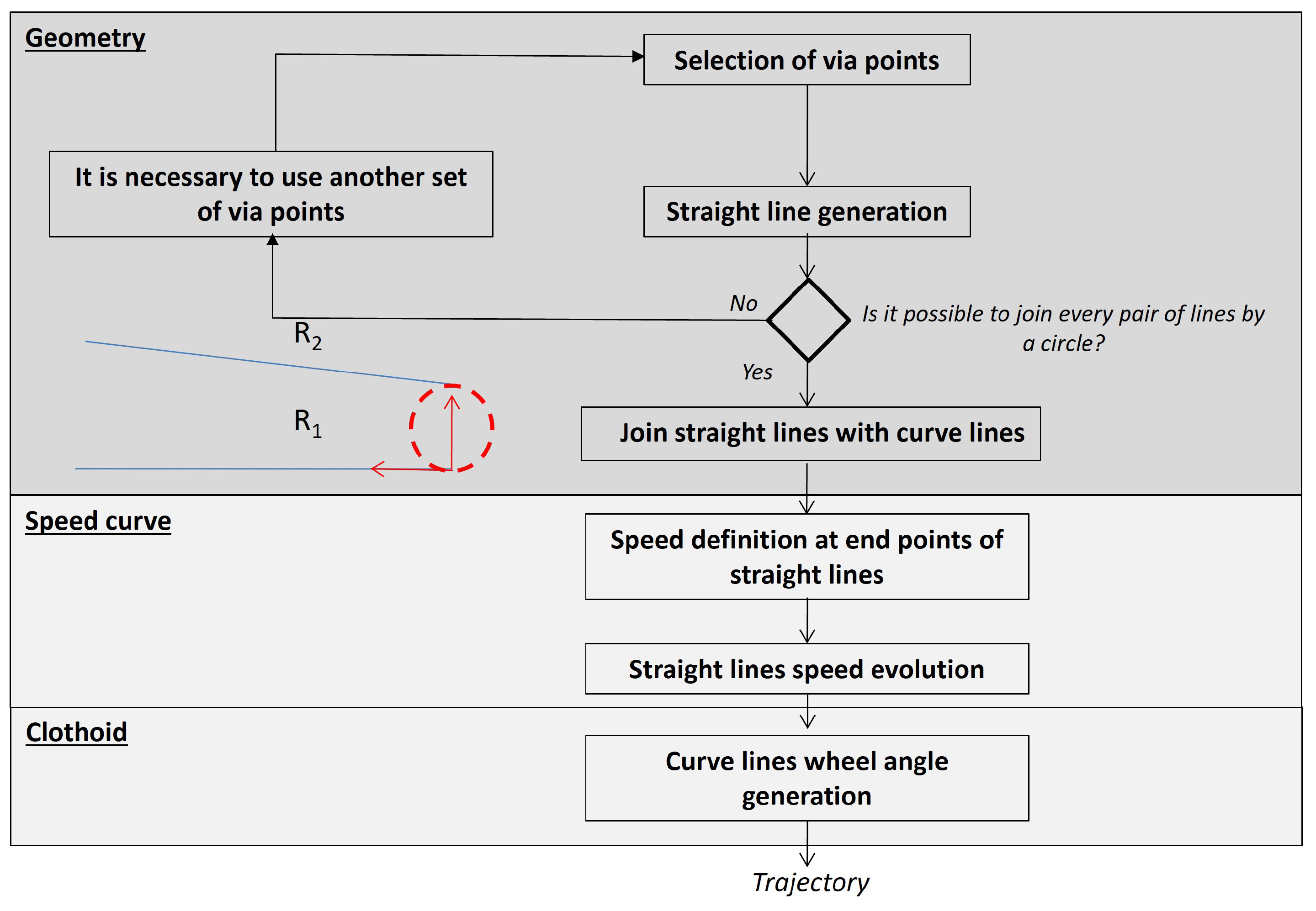
The trajectory is generated by using the algorithm described in [15] and summarized in Figure 5. The trajectory connects the guide points by using straight lines, turns, and clothoids for smoother transitions. The reference speeds at the beginning and end of the straight segment are set based on the maximum lateral acceleration allowed during curves, which maintains a constant speed. When those speeds differ, the segment is divided into acceleration, constant-speed, and deceleration sections. The trajectory planner provides the reference trajectory variables in real time. However, this transmission is paused if the relative angle compensator takes control. Once the vehicle and trailer are realigned, the tracking process is resumed.
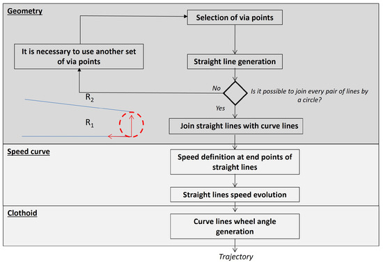
Figure 5.
Algorithm for generating the trajectory.
5. Virtual Validation
The control structure in Figure 4 was evaluated under virtual conditions using Matlab Simulink.
Validation was performed under three different conditions: a forward maneuver without and with perturbation and a backward maneuver. In forward movements, it is necessary to force a perturbation to cause jack-knifing, which naturally appears in the backward movement. The objective is to prove the functionality of the controller with and without jack-knifing conditions.
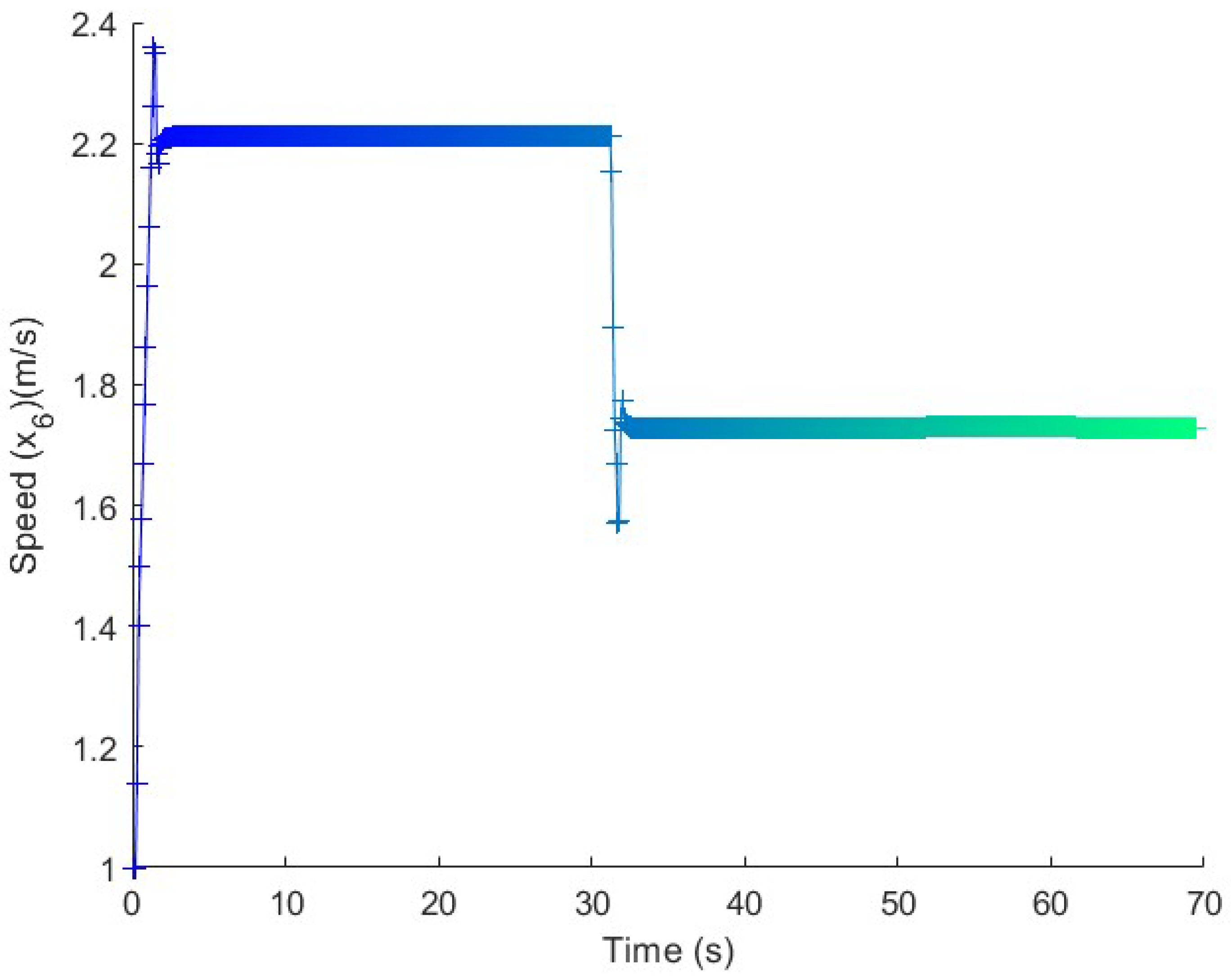
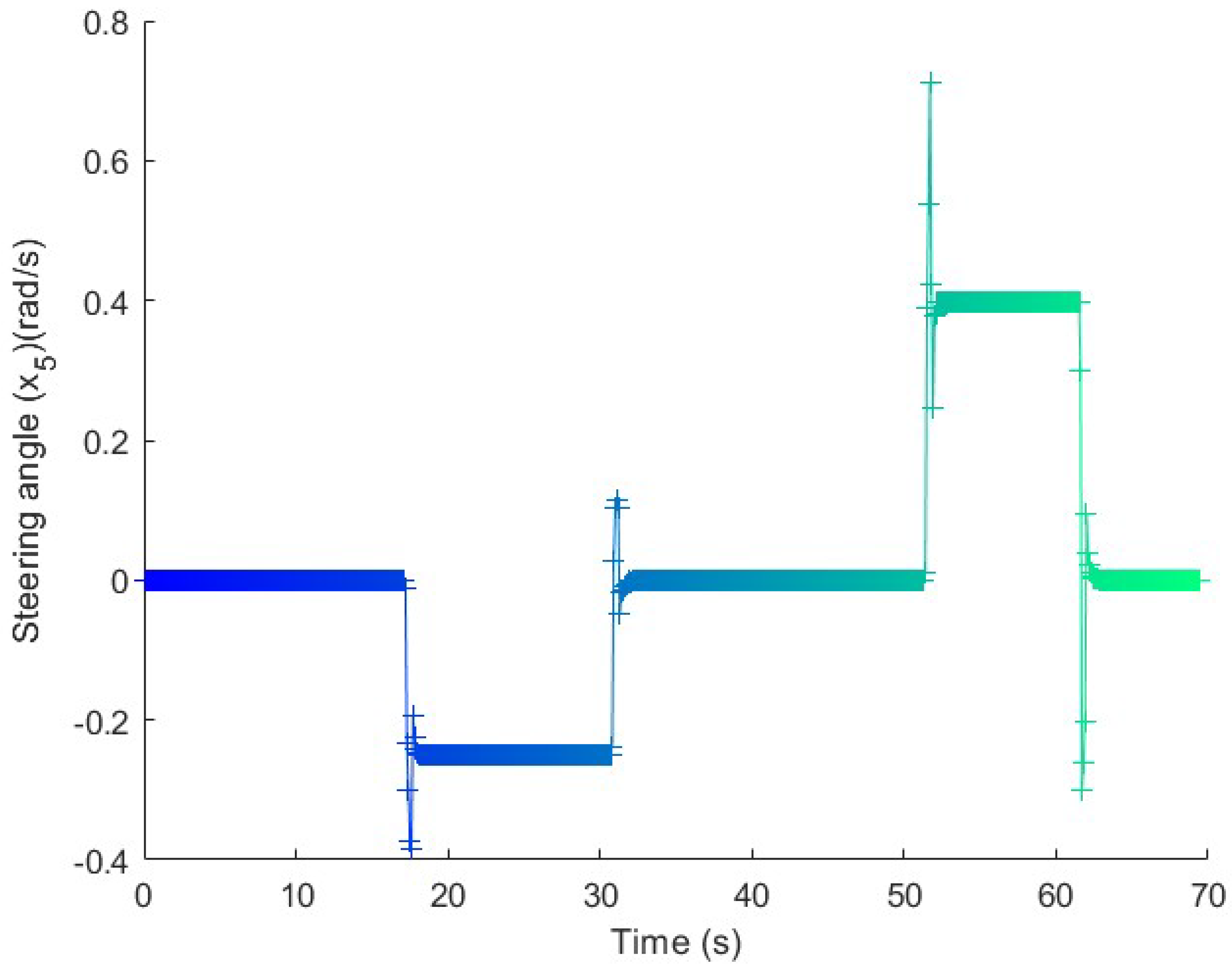
First, a long forward trajectory maneuver in the absence of perturbation is tested. The followed trajectory appears in Figure 6, where the color of the line corresponds to the time evolution. This same color pattern can be seen in the pictures of orientation (Figure 7), speed (Figure 8), and steering command (Figure 9). Figure 8 shows that the system tries to keep constant speed at the curves. The change of orientation in Figure 7 corresponds to the steering commands in Figure 9.
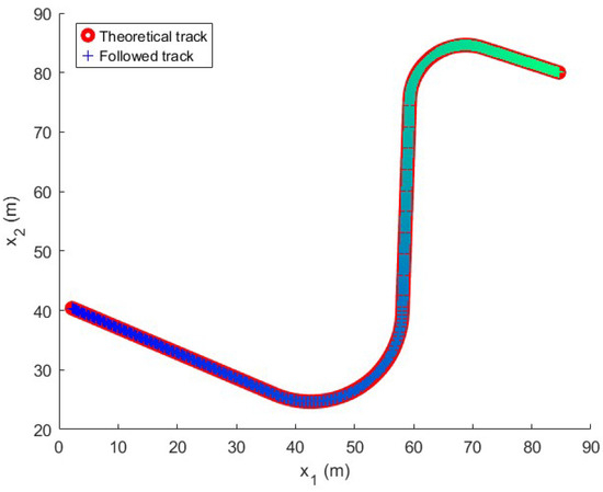
Figure 6.
Followed trajectory in the long maneuver test. The figure shows the reference in red and the followed path with a color pattern that evolves over time to relate the track point to the variable evolution in the following figures, which maintain the same color pattern.
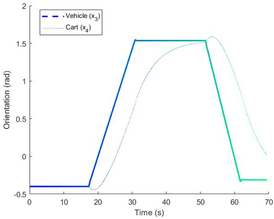
Figure 7.
Orientation in the long maneuver test. The orientations of the vehicle and cart are represented in the figure for comparison.

Figure 8.
Speed in the long maneuver test. The speed is adapted along the straight lines and kept constant in the turns.
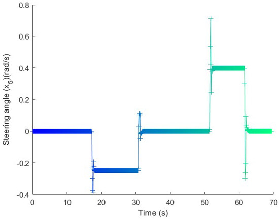
Figure 9.
Steering in the long maneuver test. The angle is kept constant along the straight line and the curves, with an adaptation range at the beginning of the turn.
After that, a perturbation is forced at the 20 s when the vehicle slides. This effect simulates a change in the friction between the road and wheels caused by variations in the road conditions—for example, the presence of water. The sliding effect is simulated by a perturbation of 2.5 rad/s in the vehicle’s angular speed () for 2 s. In absence of the relative compensator, Figure 10 shows that the vehicle cannot effectively maintain the trajectory, and it considerably deviates from the reference track marked in red. This is caused by the combined effect of the sliding at the wheels and the perturbation from the rear trailer. As observed in Figure 11, the relative angle is larger than rad, which is physically impossible, as the trailer would collide with the vehicle. The speed and steering-angle evolution are represented in Figure 12 and Figure 13.
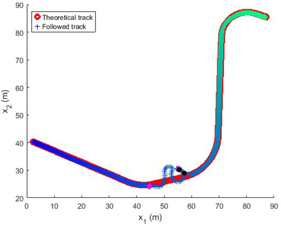
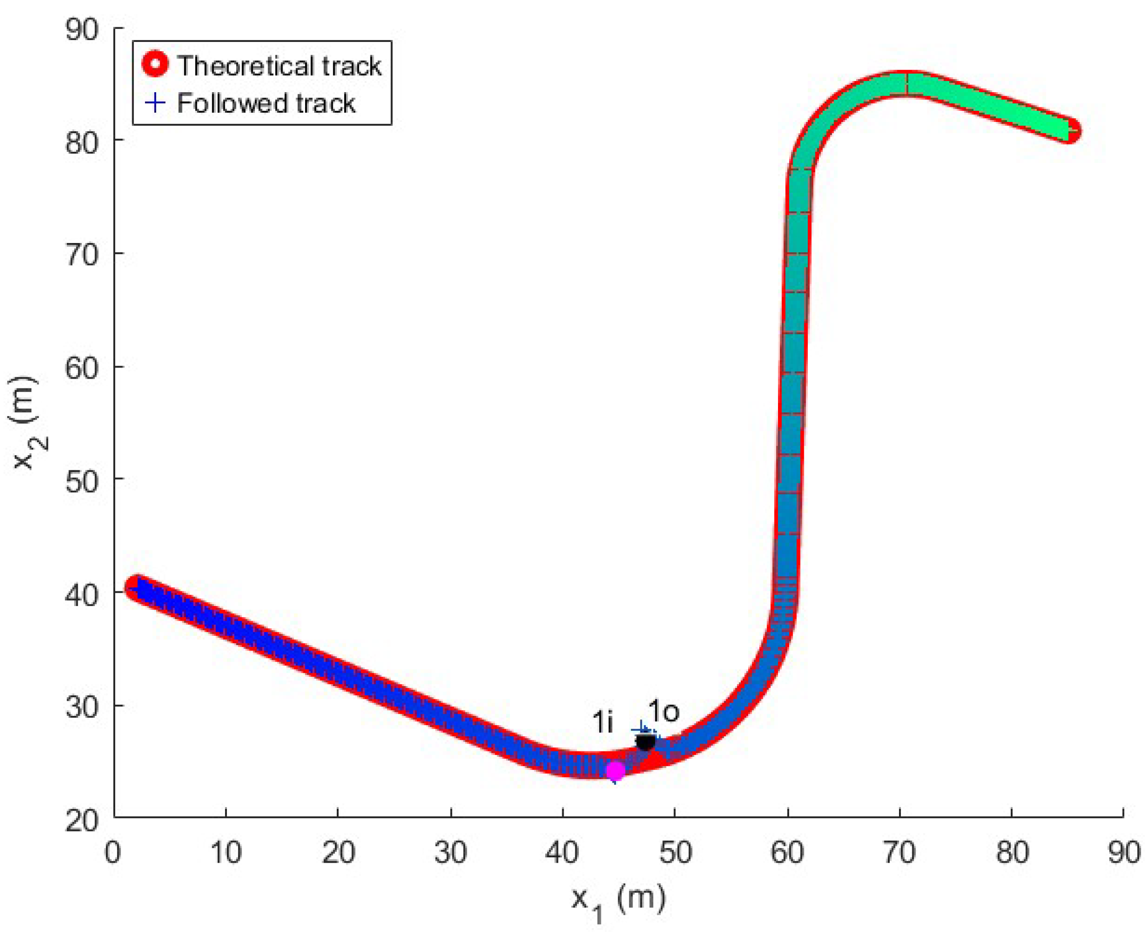
Figure 10.
Followed trajectory in the long maneuver test without a compensator. The pink and black dots represents the instants at which the relative angle compensator would have been activated and deactivated, respectively, if it were in operation.
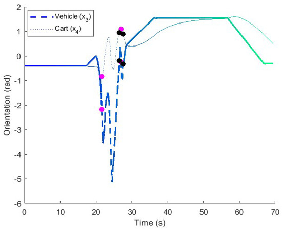
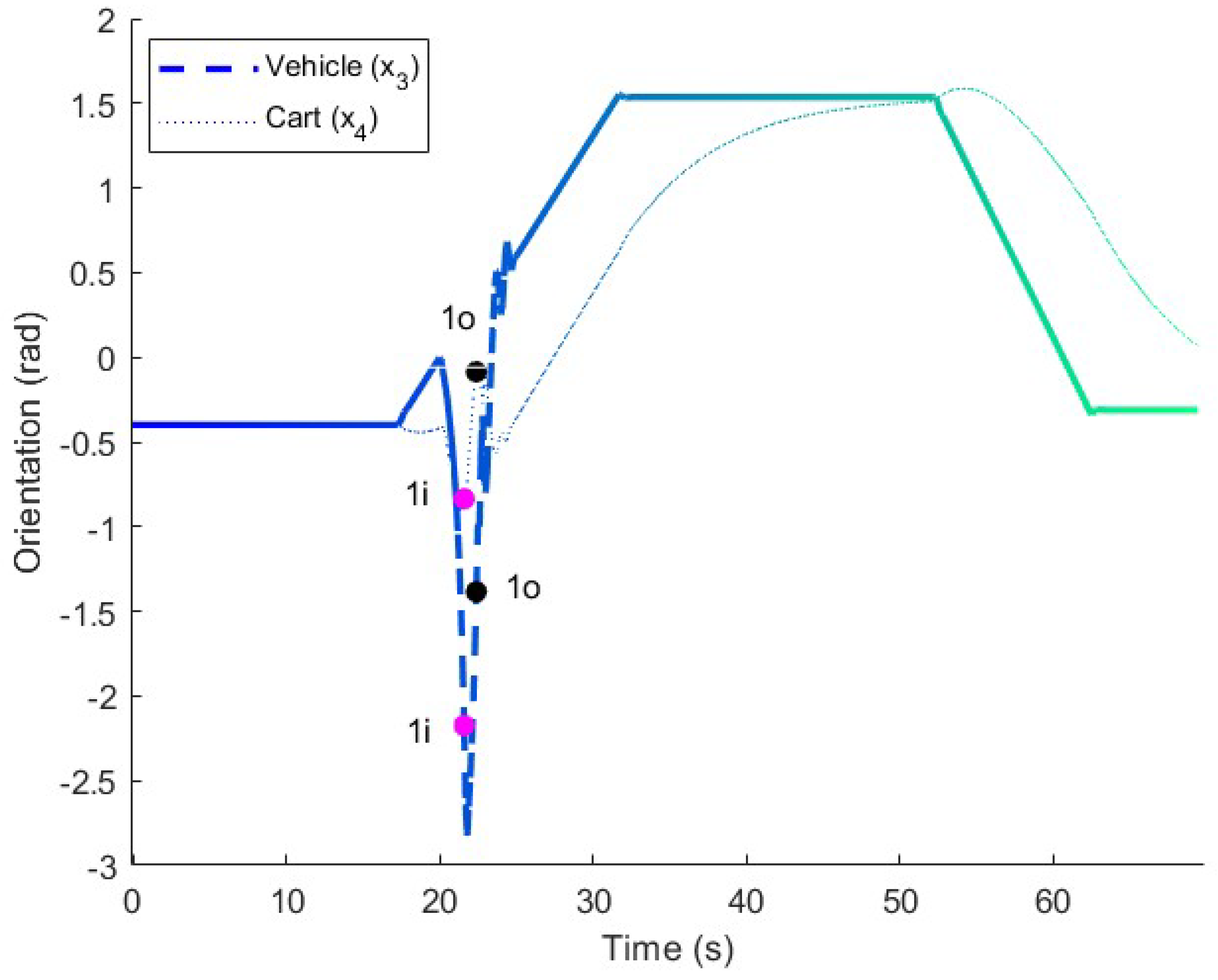
Figure 11.
Orientation in the long maneuver test without a compensator. In the absence of the relative angle compensator, the vehicle and trailer exceed the rad relative angle, which is physically impossible. The pink and black dots represents the instants at which the relative angle compensator would have been activated and deactivated, respectively, if it were in operation.

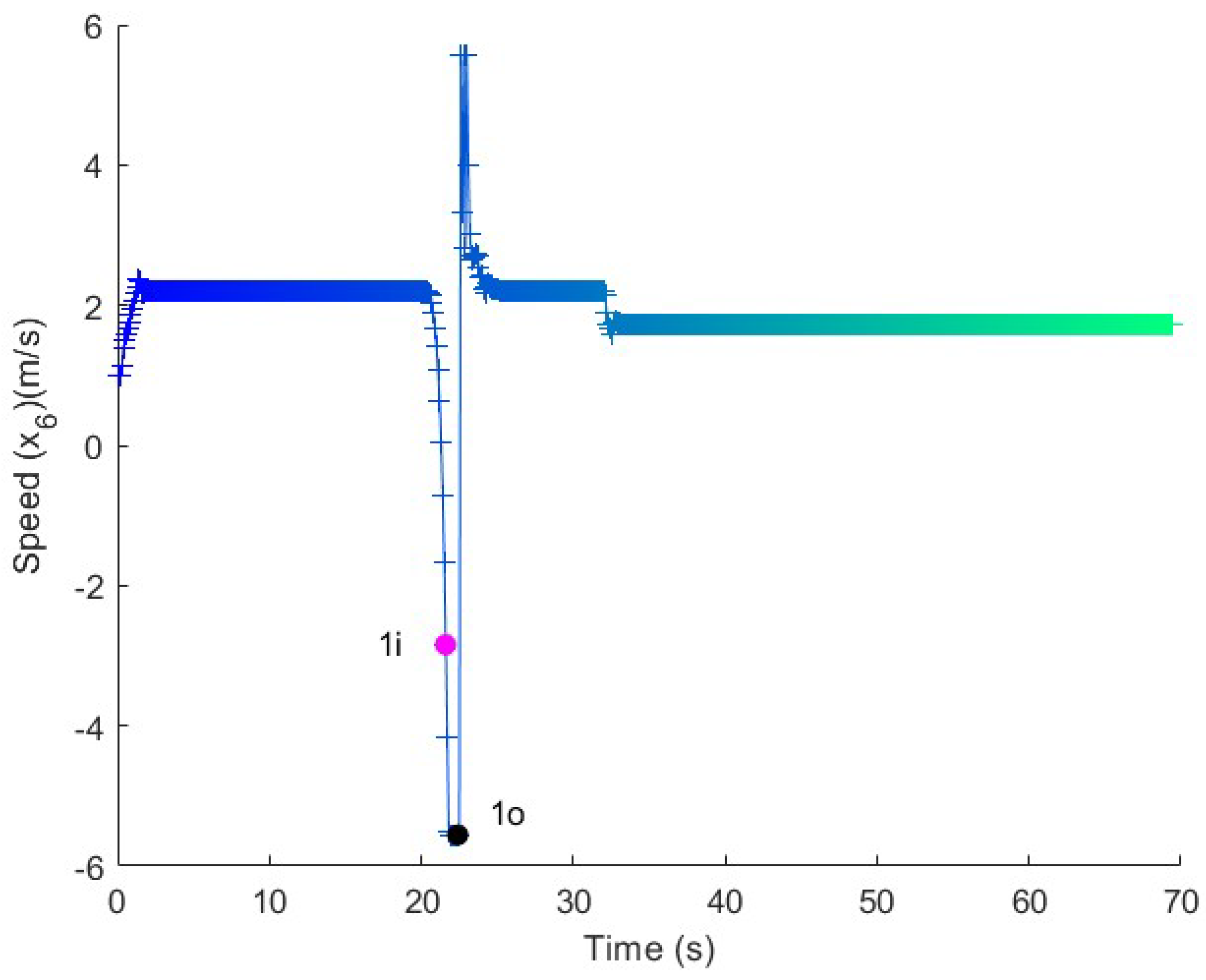
Figure 12.
Speed in the long maneuver test without a compensator. Between 21 s and 27 s, the vehicle speed is high, and it takes a long time to recover from the perturbation.The pink and black dots represents the instants at which the relative angle compensator would have been activated and deactivated, respectively, if it were in operation.

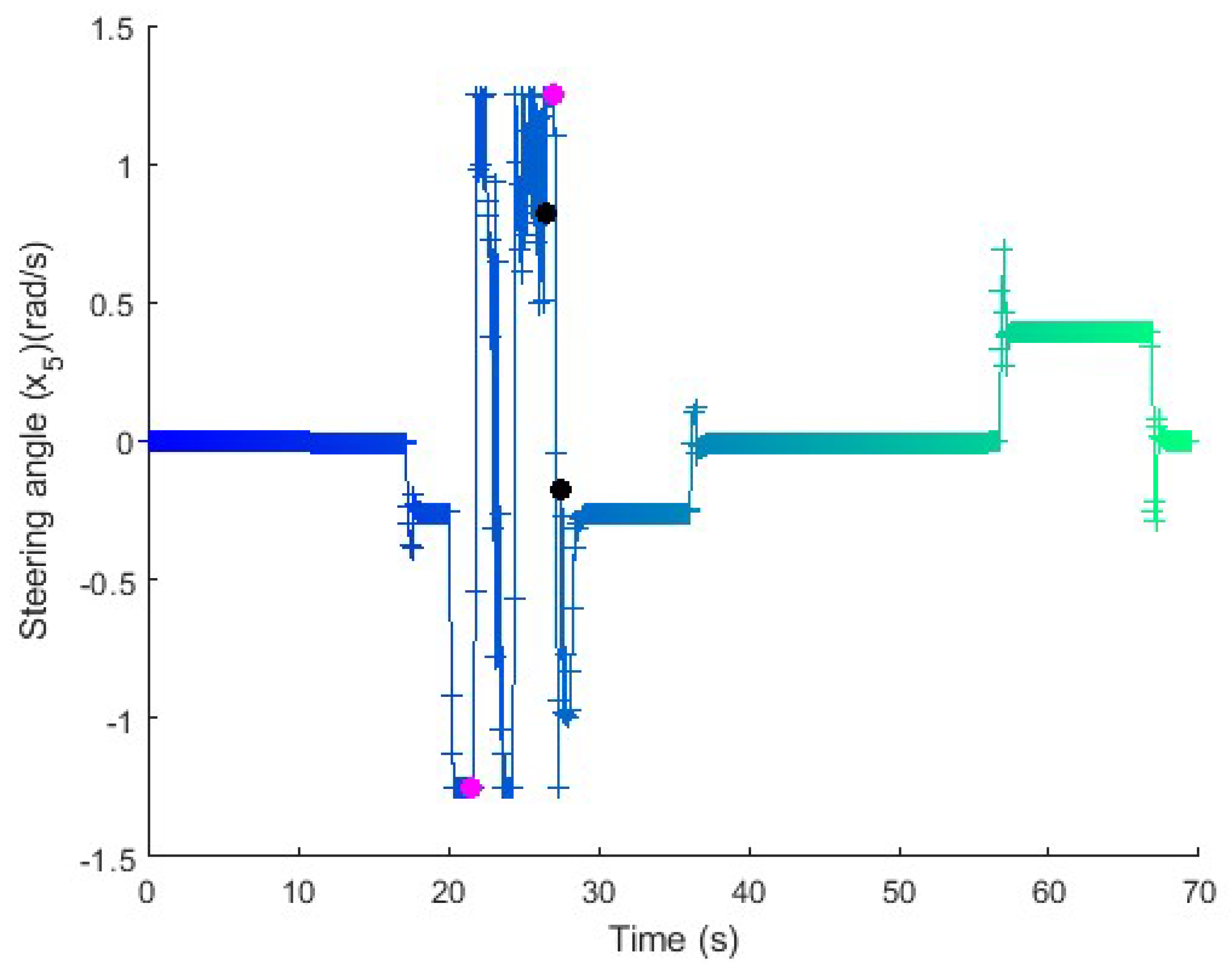
Figure 13.
Steering in the long maneuver test without a compensator. The steering command is much less smooth than the one without perturbation. The pink and black dots represents the instants at which the relative angle compensator would have been activated and deactivated, respectively, if it were in operation.
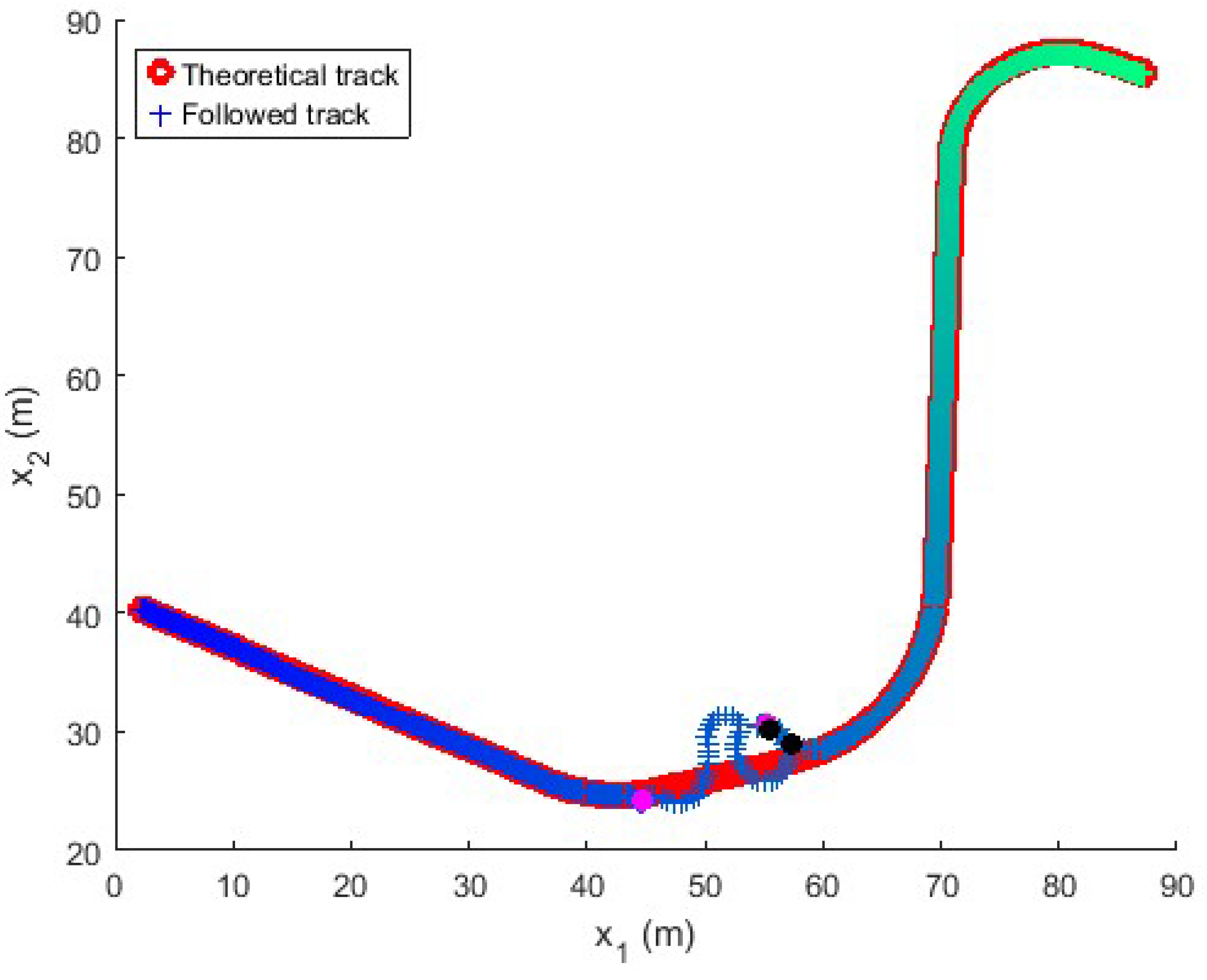
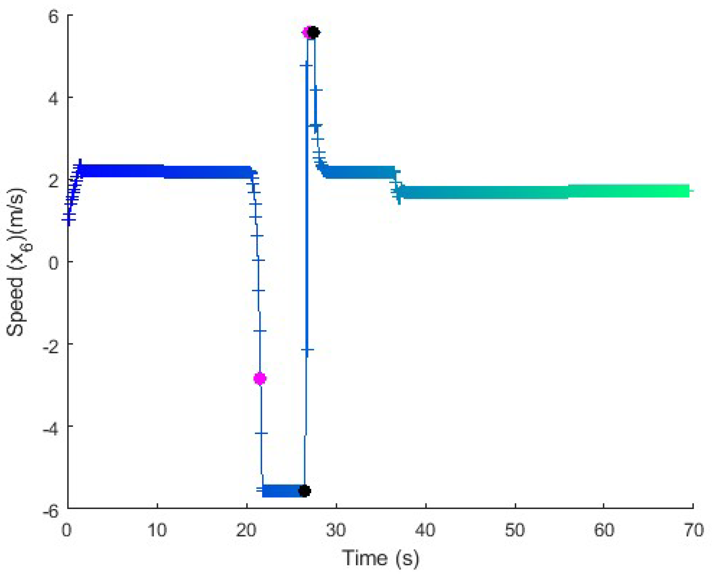
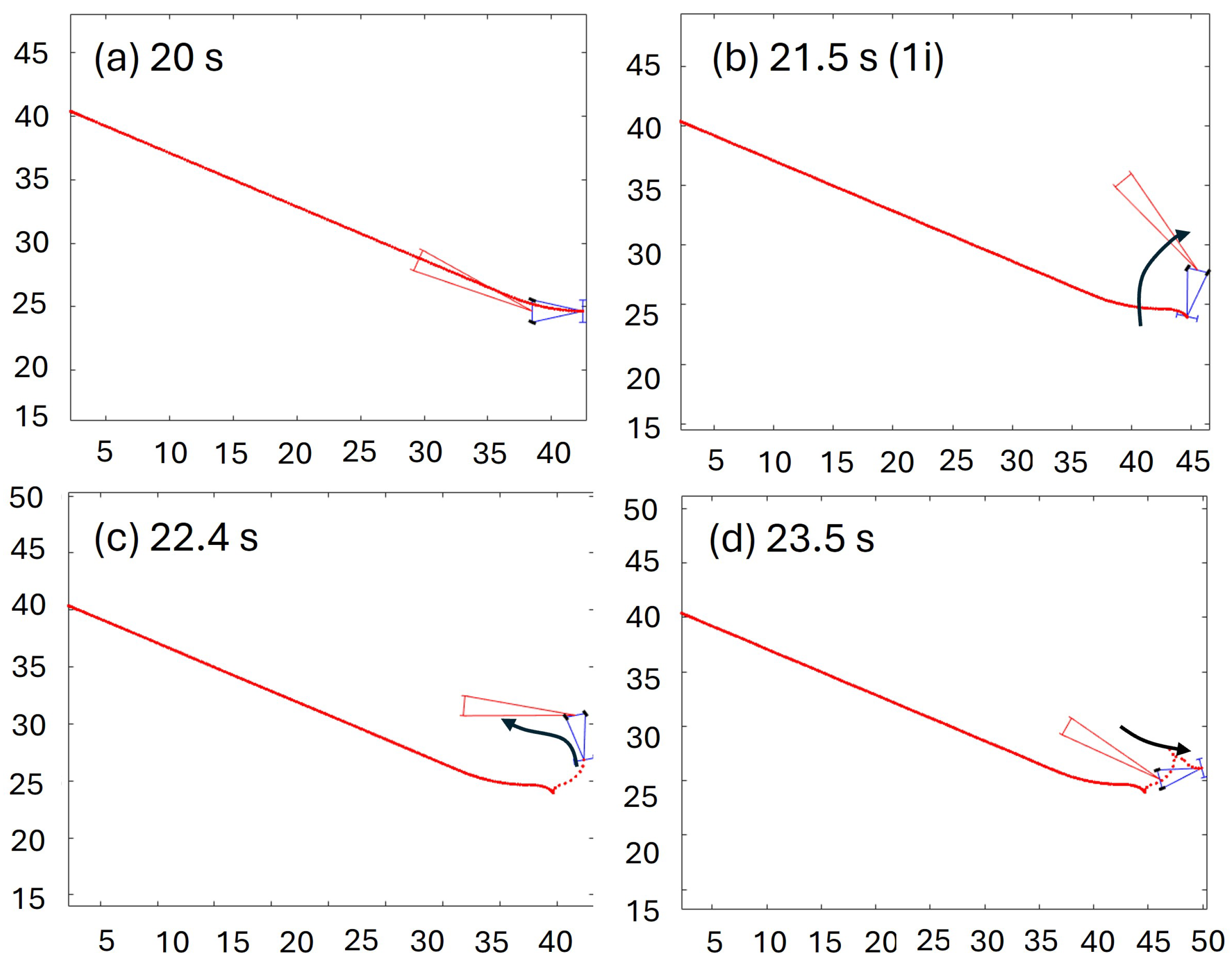
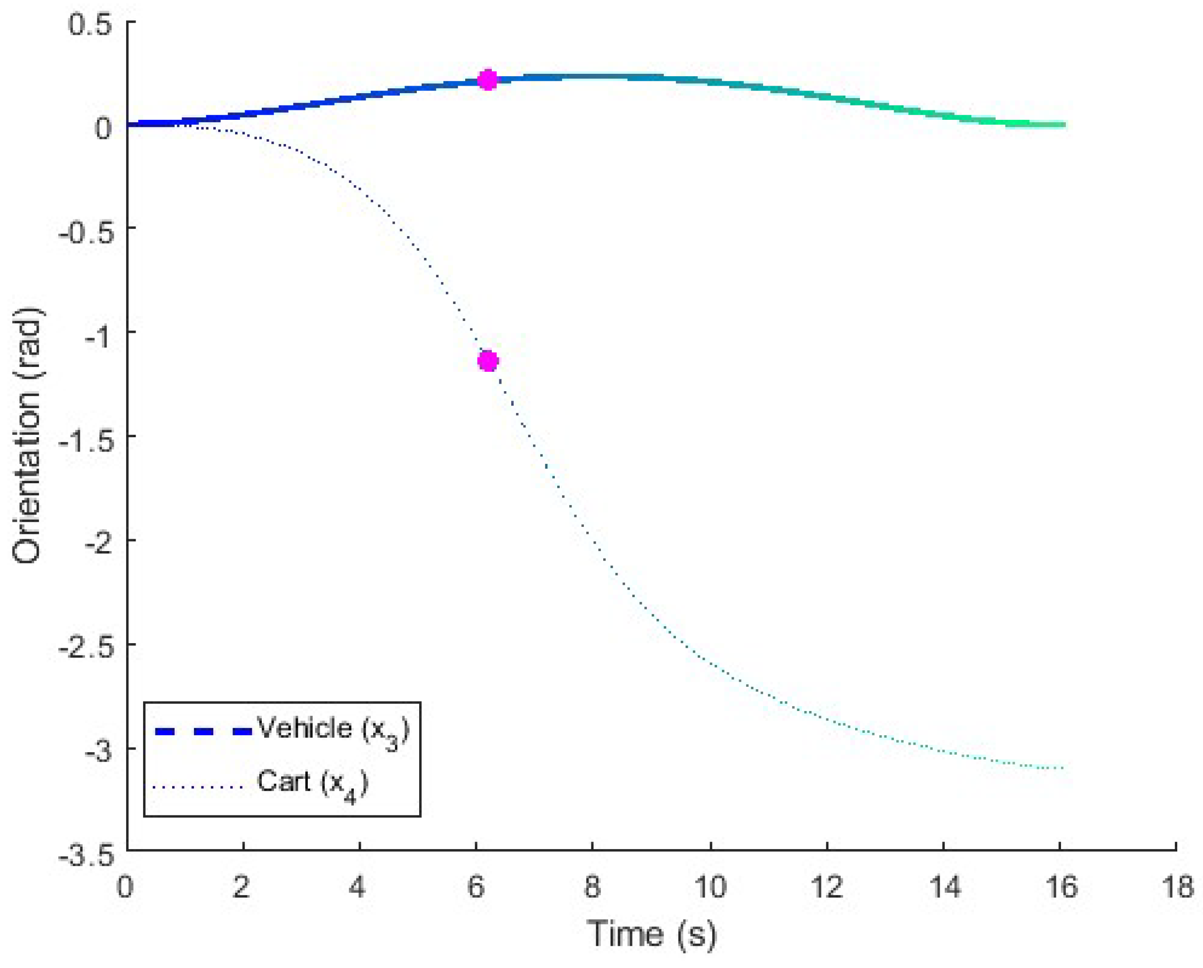
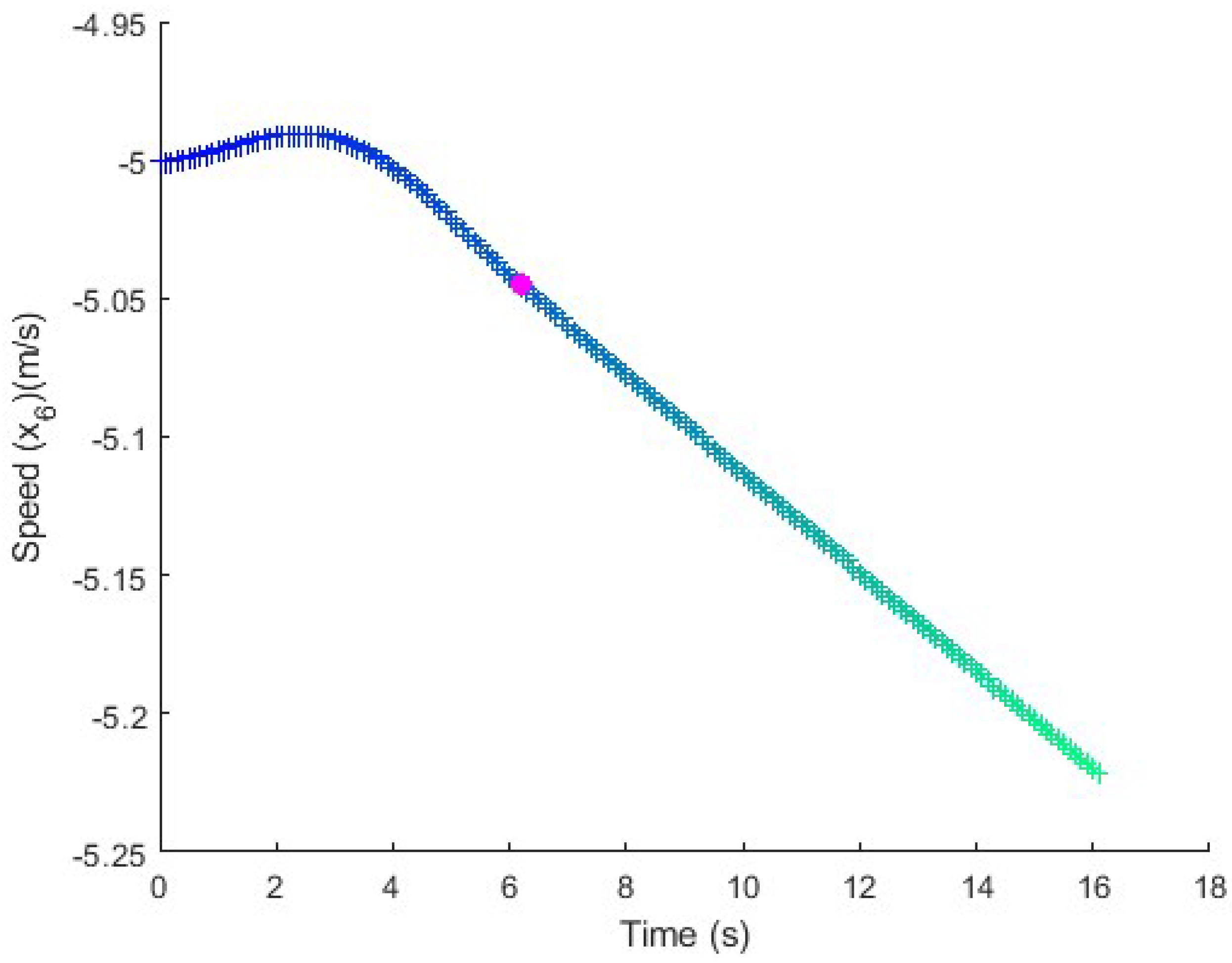
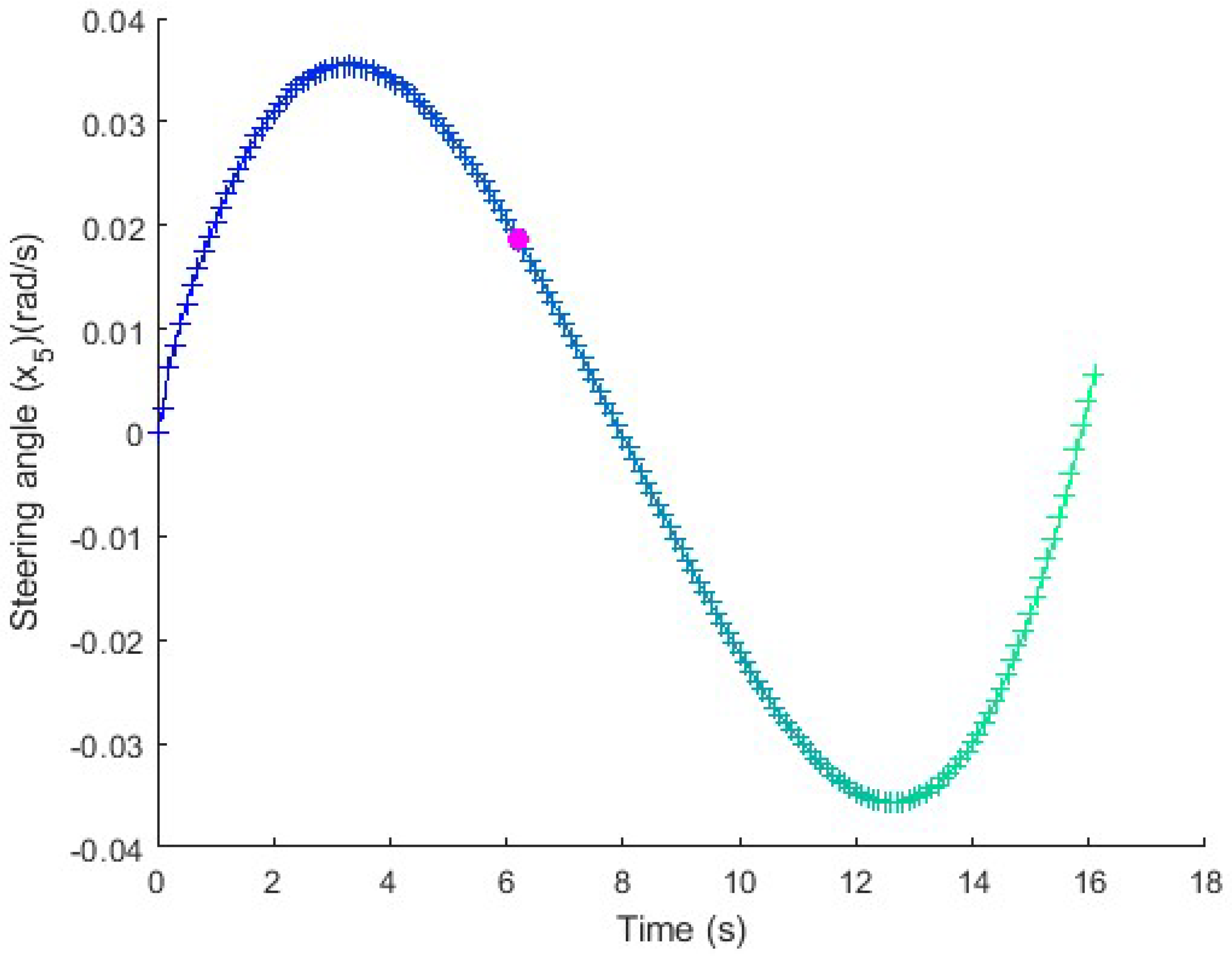
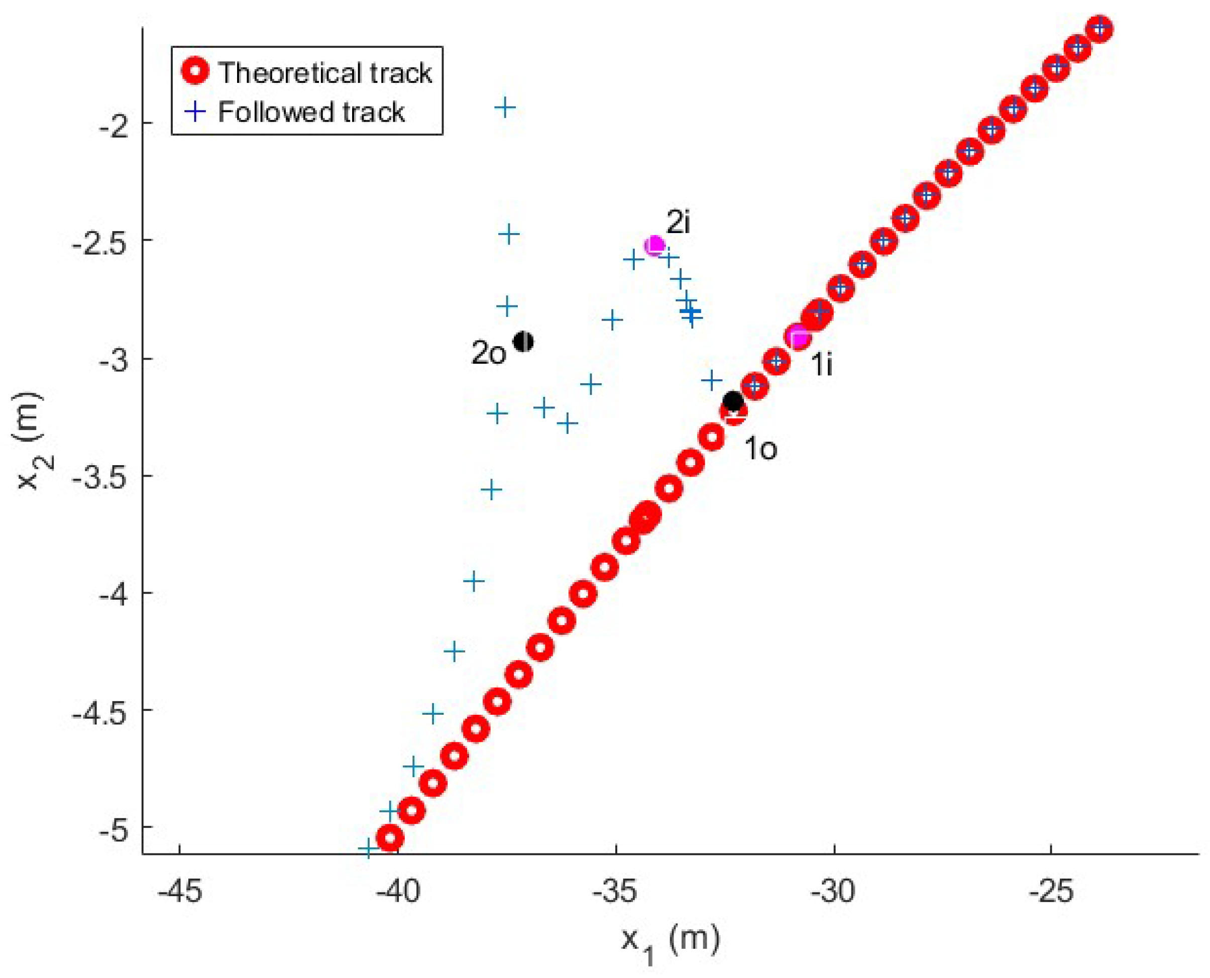
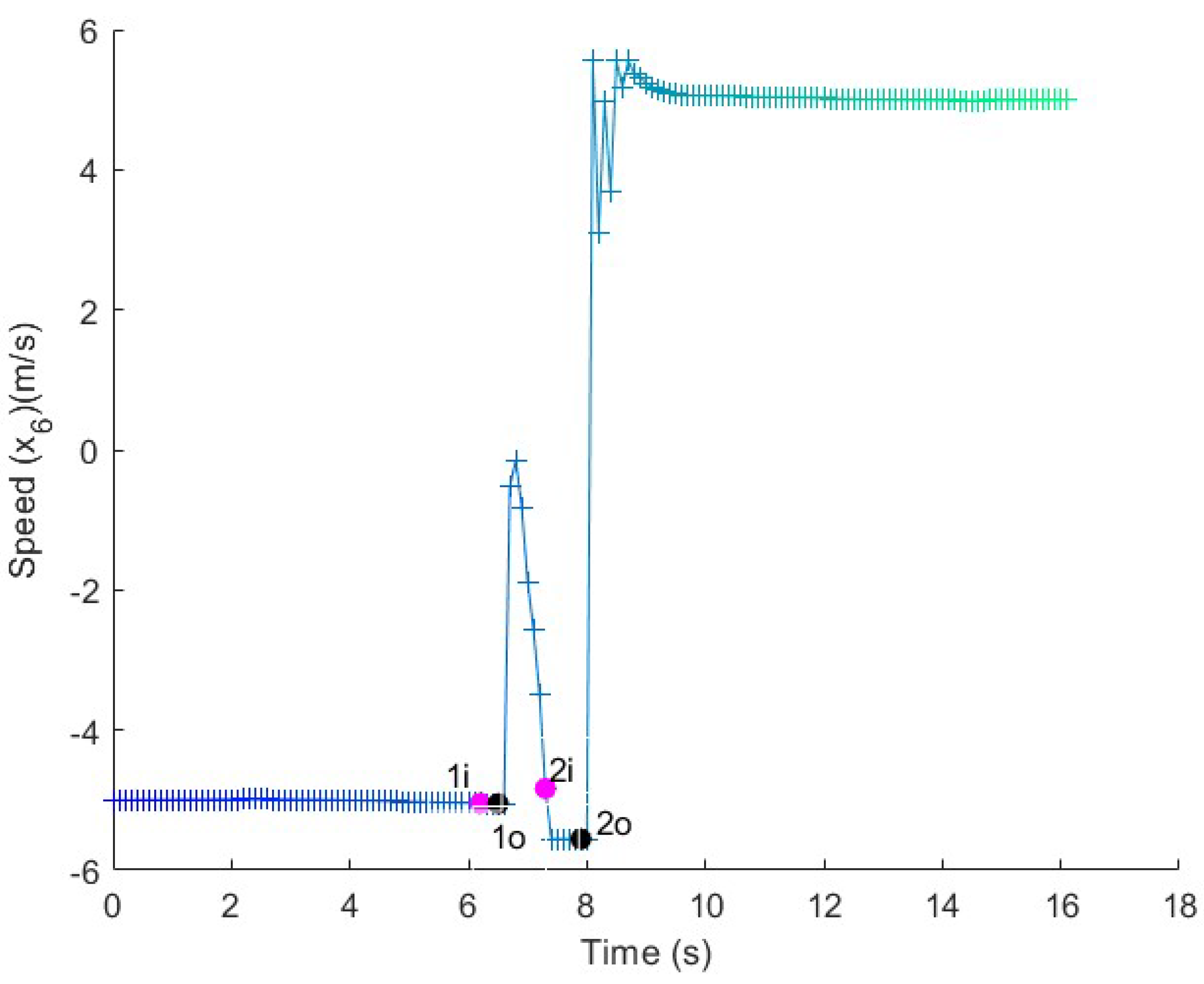
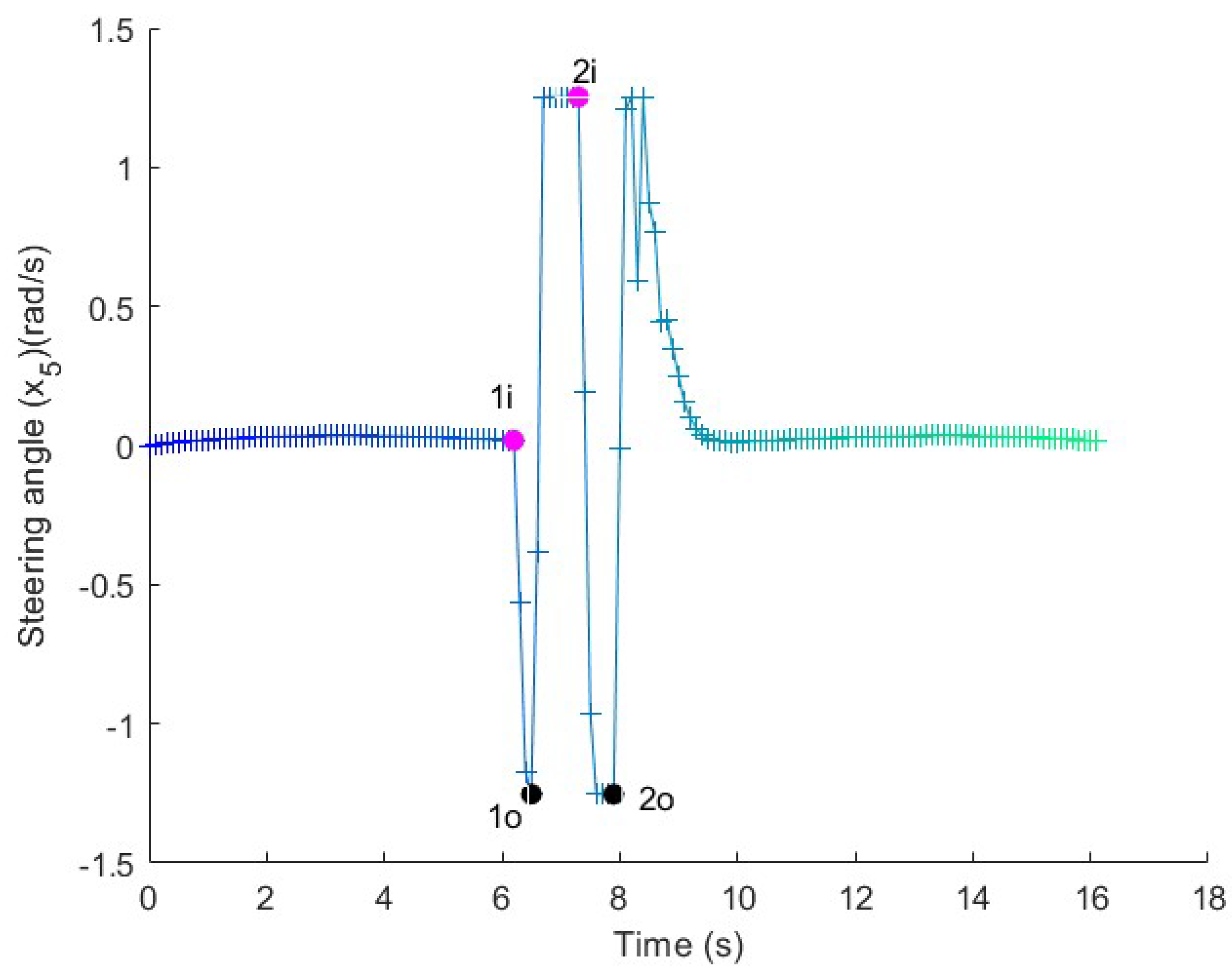
The same test is repeated with the relative angle compensator. As a consequence of the vehicle sliding, the vehicle trajectory changes, and the trailer tends to jack-knife, as can be seen in Figure 14 and the detail in Figure 15. The marks in the figure show the points at which the relative angle compensator turns on () and off (). A comparison of Figure 16 and Figure 7 shows the abrupt orientation variations in the vehicle and trailer caused by the sliding of the vehicle. At point , the relative angle exceeds the threshold of 1.3 rad, and the relative angle compensator takes over control of the vehicle. At that moment, the vehicle’s speed is kept constant, as shown in Figure 17, and the driver changes the sense of the steering command to avoid jack-knifing (Figure 18). A detailed representation of the maneuver appears in Figure 19. Both the speed and steering maneuvers are softer and shorter than without a compensator (Figure 12 and Figure 13). Just before the vehicle starts sliding at 20 s, the vehicle and trailer follow the desired trajectory. When the wheels lose adherence, both the vehicle and trailer start turning, and the relative angle compensator activates at s. At that moment, the vehicle goes backwards, turning the steering wheel to align the trailer, after which the vehicle restarts forward movement to follow the trajectory.

Figure 14.
Followed trajectory in the long maneuver test with perturbation. The figure shows the reference in red and the followed path with a color pattern that evolves over time to relate the track point to the variable evolution in the following figures, which maintain the same color pattern. (pink dot) and (black dot) represent the points at which the relative angle compensator starts and stops.
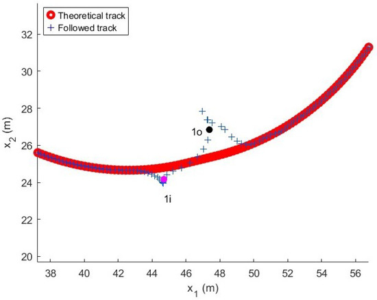
Figure 15.
Detail of the followed trajectory in the long maneuver test with perturbation. Point (pink dot) shows that before the relative angle compensator starts, the vehicle has already deviated from its trajectory due to the movement of the trailer. Point (black dot) shows the moment at which the relative angle compensator returns control to the trajectory follower.

Figure 16.
Orientation in the long maneuver test with perturbation. Points and show the start and stop moments of the relative angle compensator in the orientation of the trailer and the vehicle. The relative angle is reduced during the compensation maneuver. The pink and black dots represents the instants at which the relative angle compensator have been activated and deactivated, respectively.

Figure 17.
Speed in the long maneuver test with perturbation. Once the relative angle compensator starts, the speed tends toward a constant value. The pink and black dots represents the instants at which the relative angle compensator have been activated and deactivated, respectively.
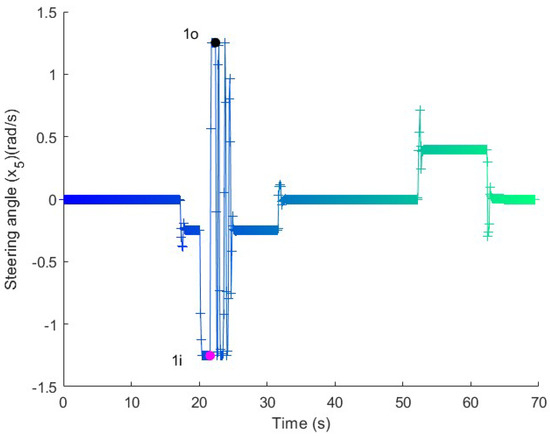
Figure 18.
Steering in the long maneuver test with perturbation. The relative angle compensator tends to counter maneuver the steering wheel to reduce the relative angle. The pink and black dots represents the instants at which the relative angle compensator have been activated and deactivated, respectively.
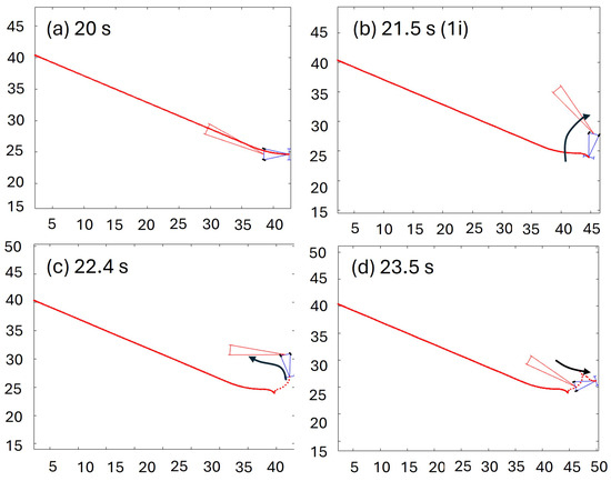
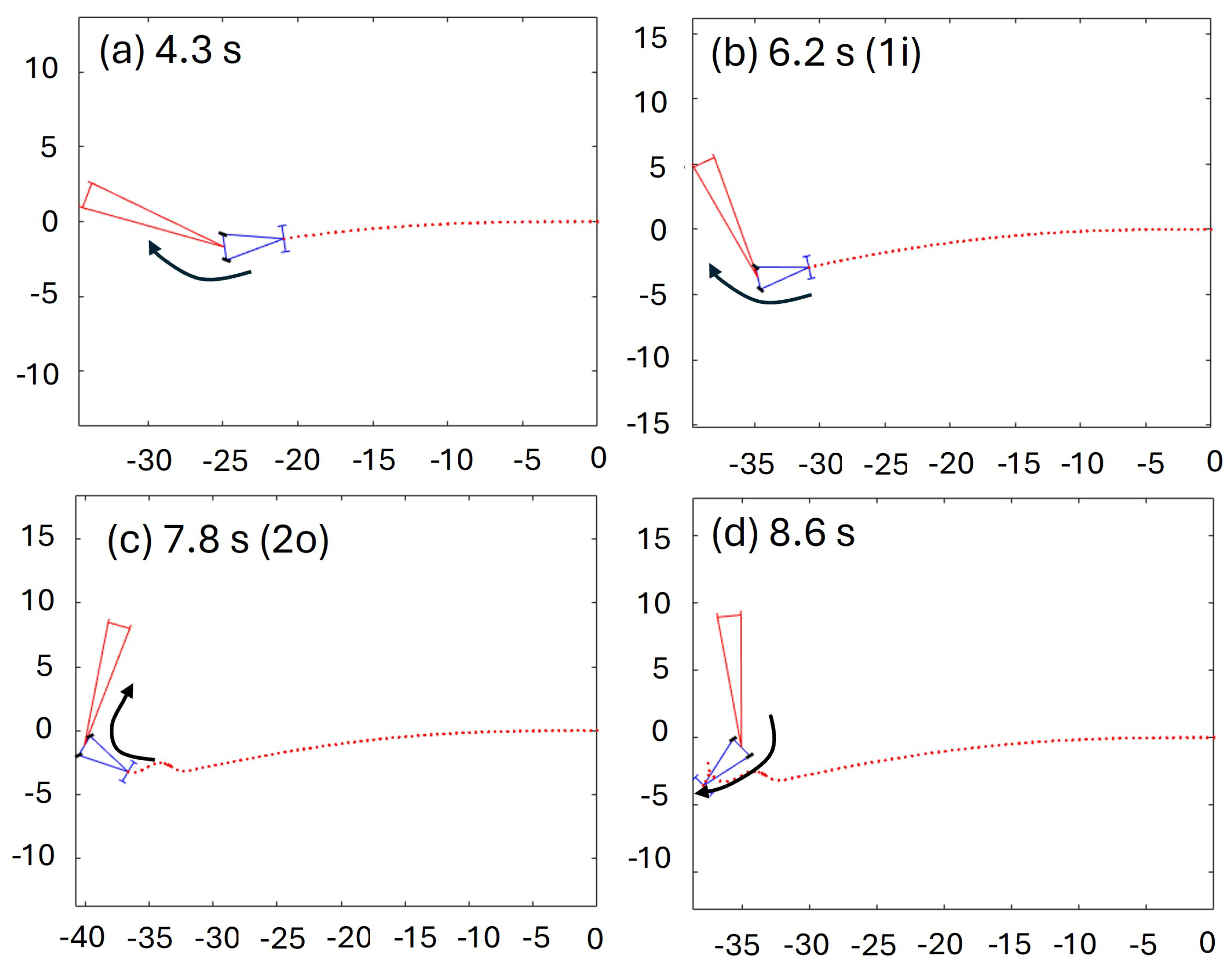
Figure 19.
Detailed representation of the maneuver in the long maneuver test with perturbation (vehicle in blue and trailer in red). (a) The vehicle follows the trajectory with a small relative angle between the vehicle and trailer; (b) the compensator activates at 21.5 s due to the perturbation; (c) the compensator moves the vehicle backwards to compensate for the angle; (d) once the vehicle and trailer are aligned, the vehicle restarts movement in the forward sense.
In the case of the backward maneuver, the trailer naturally tends to jack-knife without the presence of any perturbation as described in Equation (23). In the absence of the relative angle compensator, the path seems to be well tracked (Figure 20). However, as shown in Figure 21, the evolution of the relative angle starts increasing at the very beginning of the test, and it is about rad during the trajectory. This is an undesired behavior, as the trailer would collide with the vehicle. The evolution of the speed and steering commands is shown in Figure 22 and Figure 23. As the steering command angle in Figure 23 is positive for a long time, the relative angle increases too much and results in a collision between the vehicle and trailer at rad.
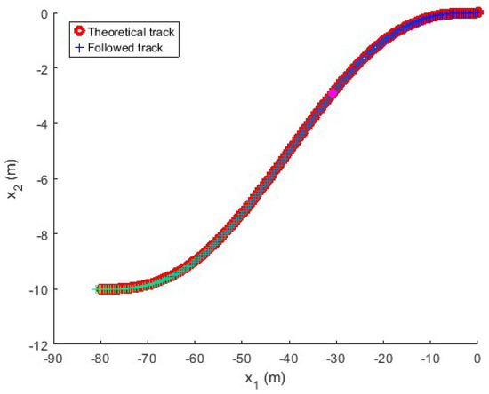
Figure 20.
Followed trajectory in the long maneuver test without a compensator. The pink dot shows that the relative angle compensator would have started operation very early during trajectory tracking.
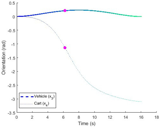
Figure 21.
Orientation in the long maneuver test without a compensator. The difference between the two curves shows a relative angle of almost rad during most of the trajectory, which implies a collision between the vehicle and trailer. The pink dot shows the instant at which the relative angle compensator would have started operation if it would be present.
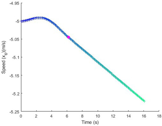
Figure 22.
Speed in the long maneuver test without a compensator. The speed evolution shows a very constant tendency along the whole trajectory because the controller does not try to compensate for the relative angle at any moment, which results in the collision between the vehicle and trailer. The pink dot shows the instant at which the relative angle compensator would have started operation if it would be present.
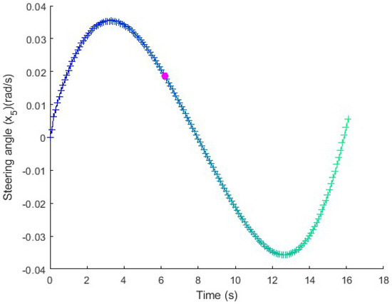
Figure 23.
Steering in the long maneuver test without a compensator. The steering evolution does not show any countermeasure to compensating for the excessive relative angle. The pink dot shows the instant at which the relative angle compensator would have started operation if it would be present.
When repeating the test with the relative angle compensator, the vehicle maneuvers to reduce the angle between the vehicle and trailer, as shown in Figure 24 and the detail in Figure 25. In this case, the relative angle compensator enters into operation twice during the test. Therefore, there are four marks in the figure for the first (, ) and second activations (, ). In both actuations of the compensator, the speed is kept constant (Figure 26). As observed in Figure 27, during the fist activation, the compensation just slightly steers the vehicle to compensate for the increase in the relative angle, but it does not affect the trajectory tracking. Just before the second actuation, the relative angle tends to sharply increase, and the vehicle gets out of the reference track. The corrective steering maneuver reduces the relative angle (Figure 28). The 2D movement of the vehicle can be seen in Figure 29. At s, the trailer has already started to turn. This trend continues until the relative angle threshold is overcome at s. The relative angle compensator continues the backwards movement to align the vehicle and the trailer and, after that, the vehicle continues trajectory tracking in the forward direction.
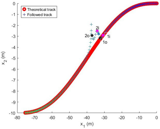
Figure 24.
Followed trajectory in the backward maneuver test. The figure shows the reference in red and the followed path with a color pattern that evolves over time to relate the track point to the variable evolution in the following figures, which maintain the same color pattern. In this case, the relative angle compensator is activated and deactivated twice, at (pink dots) and (black dots), respectively.

Figure 25.
Detail of the followed trajectory in the forward maneuver test. The first activation () is a short compensation with a minimal effect on the trajectory. The second one () shows a more drastic tracking error caused by the relative angle. The pink and black dots represents the instants at which the relative angle compensator have been activated and deactivated, respectively.
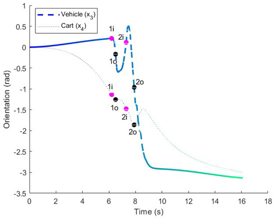
Figure 26.
Orientation in the backward maneuver test. The difference between the angles of the trailer and vehicle is lower after the actuation of the relative angle compensator, as can be seen in at points compared with . The pink and black dots represents the instants at which the relative angle compensator have been activated and deactivated, respectively.

Figure 27.
Speed in the backward maneuver test. After the second actuation of the relative angle compensator (), the trajectory tracker changes the speed. The pink and black dots represents the instants at which the relative angle compensator have been activated and deactivated, respectively.
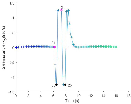
Figure 28.
Steering in the backward maneuver test. The first actuation of the relative angle compensator at shows a short actuation of the steering wheel, but the second one at results in a much larger counter-maneuver, with the steering wheel turning the complete range. The pink and black dots represents the instants at which the relative angle compensator have been activated and deactivated, respectively.
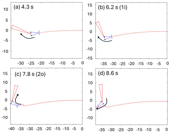
Figure 29.
Detail of the maneuver in the backward maneuver test (vehicle in blue and trailer in red). (a) From the very beginning, the trailer tends to swing with respect to the vehicle; (b) at , the relative angle is large; (c) at , the relative angle compensator turns the vehicle to align the vehicle and cart; (d) once aligned, the vehicle continues in the forward direction.
The above results show the ability of the proposed controller to follow a trajectory and react appropriately in the presence of jack-knifing conditions. In forward movements without perturbations, the trajectory tracking controller follows the reference track as desired. However, when a perturbation appears and the relative angle increases, the absence of the compensator results in collision conditions when the relative angle reaches rad values and reduced maneuverability due to the perturbations generated by the trailer. In backward movement, the trailer tends to jack-knife very early due to the instability of the movement, and a compensator is required to avoid a collision between the vehicle and trailer.
Table 3 compares the behavior of the system to the behavior of a vehicle without a trailer in the absence of external perturbations controlled using differential flatness. As can be observed, the relative angles are much lower when the relative angle compensator is activated. In fact, both forward and backward movements would be unfeasible in real conditions due to collisions between the trailer and vehicle, with angles close to rad. In the forward test, the relative angle compensator permits the system to recover faster from the sliding perturbation. In the backward test, although the time delay is null in the absence of a relative angle compensator, this is caused by the controller not avoiding the collision between vehicle and trailer, which is not a feasible solution.
Table 3.
Comparison of the evolution with and without a relative angle compensator. The maximum error is the longest distance between the vehicle reference point in the middle of the front axle and the theoretical trajectory, the maximum angle is the greatest difference between the vehicle and trailer orientation, and the time delay is the increased duration of the test with respect to the reference case.
6. Conclusions
The present paper describes a control design for a dumper vehicle with a trailer. The particularity of the system compared with previous works is the fact that the vehicle has its steering wheels on the rear axle. This has an important consequence in the mathematical linearization properties of the complete system, which makes it impossible to obtain analytical expressions for the flat outputs using the exiting algorithms. This is analyzed in Section 3, where a partial feedback linearization was demonstrated as an alternative for controlling the vehicle with the trailer. This linearization was used to design a trajectory tracking controller combined with a relative angle compensator to avoid jack-knifing between the trailer and vehicle. This control structure was successfully verified in virtual conditions.
The presented approach assumes the absence of slippery conditions under the wheels and the perfect tracking of the steering and vehicle speed at low-level controllers. Although the closed-loop structure adds robustness to the system, further developments with higher speeds should take these issues into account. Apart from that, other opportunities for extension of the present work include the implementation of the presented control architecture in a real dumper (Figure 1). The developed hardware structure is described in Section 2.2. In addition to that, further activities will include a tighter relationship between the control and the planning algorithms so that the latter updates the reference trajectory once the relative angle compensator has been activated, as well as the evaluation of potential strategies for modifying the speed when the relative angle compensator starts working. The latter can be important when the vehicle runs fast in jack-knifing conditions. This is not the case for the current application, but it could be useful for extending the present approach to other fields. Finally, the mathematical derivation for the partial linearization can be extended to conditions where the joint between the trailer and vehicle does not lie on the rear axle, which seems to be a more general condition for different vehicles and configurations.
Author Contributions
Conceptualization, R.H. and J.-M.R.-F.; methodology, J.F. and J.-M.R.-F.; software, J.-M.R.-F. and R.H.; validation, R.H.; formal analysis, J.F. and J.-M.R.-F.; investigation, J.F. and J.-M.R.-F.; resources, R.H.; data curation, R.H.; writing—original draft preparation, J.F., R.H. and J.-M.R.-F.; writing—review and editing, J.F., R.H. and J.-M.R.-F.; visualization, J.F., R.H. and J.-M.R.-F.; supervision, J.F.; project administration, J.-M.R.-F.; funding acquisition, R.H. and J.-M.R.-F. All authors have read and agreed to the published version of the manuscript.
Funding
The present work was developed within the framework of the national project titled SAFEPIT: Digital, multi-scale and autonomous slope monitoring system for a sustainable, competitive, and safe mining industry (CPP2021-008755).
Data Availability Statement
The virtual results are obtained in simulation run using Matlab Simulink software. The raw data used for the paper is not uploaded to any repository but it can be reproduced using the information summarized in the present paper.
Conflicts of Interest
The authors declare no conflicts of interest.
Abbreviations
The following abbreviations are used in this manuscript:
| LQ | Linear Quadratic |
| MPC | Model Predictive Control |
| PI | Proportional Integral |
| GPS | Global Positioning System |
| IMU | Inertial Measurement Unit |
References
- Rouchon, P.; Fliess, M.; Levine, J.; Martin, P. Flatness and motion planning: The car with n trailers. In Proceedings of the ECC’93, Groningen, The Netherlands, 28 June–1 July 1993; Volume 93, pp. 1518–1522. [Google Scholar]
- Rouchon, P.; Fliess, M.; Levine, J.; Martin, P. Flatness, motion planning and trailer systems. In Proceedings of the 32nd IEEE Conference on Decision and Control, San Antonio, TX, USA, 15–17 December 1993; Volume 3, pp. 2700–2705. [Google Scholar]
- Ryu, J.C.; Agrawal, S.K.; Franch, J. Motion Planning and Control of a Tractor With a Steerable Trailer Using Differential Flatness. J. Comput. Nonlinear Dyn. 2008, 3, 031003. [Google Scholar] [CrossRef]
- Altafini, C.; Speranzon, A.; Johansson, K.H. Hybrid Control of a Truck and Trailer Vehicle. In Proceedings of the Hybrid Systems: Computation and Control, Stanford, CA, USA, 25–27 March 2002; pp. 21–34. [Google Scholar]
- Evestedt, N.; Ljungqvist, O.; Axehill, D. Path tracking and stabilization for a reversing general 2-trailer configuration using a cascaded control approach. In Proceedings of the IEEE Intelligent Vehicles Symposium (IV), Gothenburg, Sweden, 19–22 June 2016; pp. 1156–1161. [Google Scholar] [CrossRef]
- Werling, M.; Reinisch, P.; Heidingsfeld, M.; Gresser, K. Reversing the General One-Trailer System: Asymptotic Curvature Stabilization and Path Tracking. IEEE Trans. Intell. Transp. Syst. 2014, 15, 627–636. [Google Scholar] [CrossRef]
- Alipour, K.; Robat, A.B.; Tarvirdizadeh, B. Dynamics modeling and sliding mode control of tractor-trailer wheeled mobile robots subject to wheels slip. Mech. Mach. Theory 2019, 138, 16–37. [Google Scholar] [CrossRef]
- Huynh, V.T.; Smith, R.N.; Kwok, N.M.; Katupitiya, J. A nonlinear PI and backstepping-based controller for tractor-steerable trailers influenced by slip. In Proceedings of the IEEE International Conference on Robotics and Automation, Saint Paul, MN, USA, 14–18 May 2012; pp. 245–252. [Google Scholar] [CrossRef]
- Yuan, W.; Liu, Y.; Liu, Y.H.; Su, C.Y. Differential flatness-based adaptive robust tracking control for wheeled mobile robots with slippage disturbances. ISA Trans. 2024, 144, 482–489. [Google Scholar] [CrossRef]
- Sriprang, S.; Poonnoy, N.; Guilbert, D.; Nahid-Mobarakeh, B.; Takorabet, N. Design, Modeling, and Differential Flatness Based Control of Permanent Magnet-Assisted Synchronous Reluctance Motor for e-Vehicle Applications. Sustainability 2021, 13, 9502. [Google Scholar] [CrossRef]
- Bitauld, L.; Fliess, M.; Lévine, J. A flatness based control synthesis of linear systems and application to windshield wipers. In Proceedings of the 1997 European Control Conference (ECC), Brussels, Belgium, 1–4 July 1997. [Google Scholar]
- Bonnabel, S.; Claeys, X. Industrial Control of Tower Cranes An Operator in the Loop Approach. IEEE Control Syst. Mag. 2020, 40, 27–39. [Google Scholar] [CrossRef]
- Lobe, A.; Ettl, M.; Steinboeck, A.; Kugi, A. Flatness-based nonlinear control of a three-dimensional gantry crane. IFAC-PapersOnLine 2018, 51, 331–336. [Google Scholar] [CrossRef]
- Rigatos, G.; Zervos, N.; Busawon, K.; Siano, P.; Abbaszadeh, M. Differential flatness theory-based approach to the control of gas-turbine electric power generation units. IET Control Theory Appl. 2020, 14, 187–197. [Google Scholar] [CrossRef]
- Franch, J.; Rodriguez-Fortun, J.M. Control and trajectory generation of an Ackerman vehicle by dynamic linearization. In Proceedings of the 2009 European Control Conference (ECC), Budapest, Hungary, 23–26 August 2009; pp. 4937–4942. [Google Scholar] [CrossRef]
- Han, Z.; Wu, Y.; Li, T.; Zhang, L.; Pei, L.; Xu, L.; Li, C.; Ma, C.; Xu, C.; Shen, S.; et al. An Efficient Spatial-Temporal Trajectory Planner for Autonomous Vehicles in Unstructured Environments. IEEE Trans. Intell. Transp. Syst. 2024, 25, 1797–1814. [Google Scholar] [CrossRef]
- Nilsson, P.; Laine, L.; Sandin, J. High Speed Control of Long Combination Heavy Commercial Vehicles Within Safe Corridors. Driving Simulation Center. Published by VTI, Linköping 2016. Available online: https://www.diva-portal.org/smash/get/diva2:1071781/FULLTEXT01.pdf (accessed on 29 May 2025).
- Yu, C.; Zheng, Y.; Shyrokau, B.; Ivanov, V. MPC-based path following design for automated vehicles with rear wheel steering. In Proceedings of the 2021 IEEE International Conference on Mechatronics (ICM), Kashiwa, Japan, 7–9 March 2021; pp. 1–6. [Google Scholar]
- Gonzalez-Cantos, A.; Ollero, A. Backing-Up Maneuvers of Autonomous Tractor-Trailer Vehicles using the Qualitative Theory of Nonlinear Dynamical Systems. Int. J. Robot. Res. 2009, 28, 49–65. [Google Scholar] [CrossRef]
- Marino, R. On the largest feedback linearizable subsystem. Syst. Control Lett. 1986, 6, 345–351. [Google Scholar] [CrossRef]
- Pathak, K.; Franch, J.; Agrawal, S. Velocity and position control of a wheeled inverted pendulum by partial feedback linearization. IEEE Trans. Robot. 2005, 21, 505–513. [Google Scholar] [CrossRef]
- Martin, P.; Rouchon, P. Feedback linearization and driftless systems. Math. Control. Signals Syst. 1994, 7, 235–254. [Google Scholar] [CrossRef]
- Li, S.J.; Respondek, W. Flat outputs of two-input driftless control systems. ESAIM Control. Optim. Calc. Var. 2012, 18, 774–798. [Google Scholar] [CrossRef]
- Gstottner, C.; Kolar, B.; Schoberl, M. Necessary and sufficient conditions for the linearisability of two-input systems by a two-dimensional endogenous dynamic feedback. Int. J. Control 2023, 96, 800–821. [Google Scholar] [CrossRef]
- Fossas, E.; Franch, J.; Agrawal, S. Linearization by prolongations of two-input driftless systems. In Proceedings of the IEEE Conference on Decision and Control, Sydney, NSW, Australia, 12–15 December 2000; Volume 4, pp. 3381–3385. [Google Scholar] [CrossRef]
- Levine, J. Differential Flatness by Pure Prolongation: Necessary and Sufficient Conditions. arXiv 2023, arXiv:2303.17761. [Google Scholar]


Disclaimer/Publisher’s Note: The statements, opinions and data contained in all publications are solely those of the individual author(s) and contributor(s) and not of MDPI and/or the editor(s). MDPI and/or the editor(s) disclaim responsibility for any injury to people or property resulting from any ideas, methods, instructions or products referred to in the content. |
© 2025 by the authors. Licensee MDPI, Basel, Switzerland. This article is an open access article distributed under the terms and conditions of the Creative Commons Attribution (CC BY) license (https://creativecommons.org/licenses/by/4.0/).