A Configuration Method for Energy Storage Systems in Distribution Networks by Simultaneously Improving Operation Stability and Photovoltaic Hosting Capacity

Abstract

Due to the development of renewable energy and the requirement of environmental friendliness, more distributed photovoltaics (DPVs) are connected to distribution networks. The optimization of stable operation and the improvement of DPV hosting capacity are urgently needed. Energy storage systems (ESSs), as a flexible resource, show great promise in DPV integration and optimal dispatching. Thus, an optimal configuration method for ESSs is proposed. Firstly, a two-layer, double-stage configuration model of ESSs is constructed. The inner layer contains two stages of network operation optimization and DPV hosting capacity improvement. The daily cost, voltage deviation and net load fluctuation rate are optimized in the first stage. The hosting capacity of the DPV is maximized in the second stage. The position and capacity of the ESS are configured in the outer layer. Secondly, a solution strategy for the proposed model is designed. Focusing on different problem-solving intelligence algorithms, solvers and analytic hierarchy process–anti-entropy weighting methods are used for effectively selecting comprised optimal solutions. Simulations verified the effectiveness and applicability of the proposed method. This method comprehensively considers the stable operation of distribution networks and the improvement of DPV hosting capacity, which provides scientific guidance for the orderly access of DPVs in distribution networks.

1. Introduction

The global energy transition has catalyzed the unprecedented proliferation of distributed photovoltaic (DPV) deployment worldwide. The European Union’s Renewable Energy Directive establishes binding renewable energy targets [1]. The U.S. Inflation Reduction Act implements structured fiscal incentives for solar-storage hybridization [2]. China’s dual carbon policy framework vigorously promotes renewable integration [3]. However, the high-penetration integration of DPVs into active distribution networks (AND) brings significant spatiotemporal challenges [4]. The intermittency and uncertainty of DPVs may cause reverse power flow, exacerbated net load fluctuations, increased voltage deviations and reliability degradation, which threaten network operation stability [5]. Thus, the contradiction between maintaining network operation stability and large amounts of DPV integration brings worldwide attention.

Energy storage systems (ESSs) provide critical solutions for DPV integration through their unique bidirectional power regulation and temporal energy shifting capabilities [6]. Considering the interaction between source, storage and load, the collaborative optimal configuration model for minimizing economic costs is an important research direction [7]. Xie et al. [8] listed several applicable functions in practical ESS projects, including peak cutting and valley filling, renewable energy output smoothing, overvoltage suppression and harmonic oscillation suppression. Yan et al. [9] proposed a multi-stage, four-level intelligent optimization control algorithm that integrated electric vehicle charging stations with PVs and battery ESSs. The algorithm planned the optimal charging and discharging strategies for electric vehicles and battery packs to reduce distribution network operational costs and improve reliability. Liao et al. [10] proposed a bi-level optimization model for DPVs and ESSs based on an improved deep-embedded K-means clustering algorithm, with the objective of minimizing daily operation costs, voltage deviations and network losses. Rawa et al. [11] proposed a seasonal optimization framework for optimizing the short-term operations of a microgrid, including energy storage and PVs, to reduce the total operation costs of the grid-integrated microgrid. Cho et al. [12] proposed a PV-ESS optimization configuration method for ADNs, improving renewable integration and economic performance through capacity configuration. Zhang et al. [13] established a bi-level planning model for distribution networks. The aim was to minimize cost and voltage deviation. This model optimized the coordinated operation of source–grid–load–storage and determined the sitting and sizing of ESSs.

To optimize ESS configurations, researchers have developed various assessment methods. Zhou et al. [14] used a bi-level optimization model to integrate multiple renewable sources and ESSs for cost-effective and reliable distribution network planning. Li et al. [15] introduced the energy storage performance index to evaluate the importance of distributed energy storage systems in the grid, optimizing their daily operations and investment costs using a genetic algorithm. Picioroaga et al. [16] proposed a resilience-driven ESS-sizing method based on a Mixed-Integer Linear Programming model to enhance microgrid reliability and resilience, using recovery and resilience indices. Rasool et al. [17] further expanded the assessment scope by developing a multi-objective optimization framework for hybrid renewable energy systems, incorporating the renewable energy supply fraction and energy export index alongside the cost of energy to provide a comprehensive evaluation of ESS configurations.

DPV hosting capacity refers to the maximum DPV capacity that a distribution network can safely accommodate. It serves as a crucial basis for the planning and operation of ADNs. Koirala et al. [18] evaluated various deterministic and stochastic methods for calculating the hosting capacity of photovoltaic systems in low-voltage distribution networks. By using real network data, the strengths and applicability of each approach were highlighted. Tan et al. [19] established a DPV hosting capacity assessment model for medium-voltage distribution networks, with the equivalent grid-connected capacity of DPVs as the objective function. Jain et al. [20] proposed a dynamic distributed photovoltaic hosting capacity methodology that could more fully capture the grid impacts of distributed photovoltaic systems compared to traditional methods. Allocating ESSs to enhance DPV hosting capacity has been proven effective. Shabbir et al. [21] proposed a machine learning-based control solution to alleviate overloading and overvoltage issues caused by the high penetration of DPV installations in low-voltage ADNs. The strategy employs a long short-term memory algorithm for day-ahead PV forecasting to optimize the charging/discharging of residential ESSs. Zhou et al. [22] proposed an optimal configuration and charging/discharging strategy for energy storage systems to improve the hosting capacity level of DPVs. Additionally, Vellingiri et al. [23] proposed a method to estimate the maximum hosting capacity for renewables in power grids, considering both ESSs and transmission line expansion. Numerical studies demonstrated the efficiency of the proposed method in maximizing renewable energy source penetration and improving system reliability.

In summary, ESSs play a crucial role in promoting renewable energy integration and enhancing hosting capacity. However, an ESS configuration method considering both current network operation optimization and the further improvement of DPV hosting capacity has not been reported. Thus, an ESS optimal configuration method is proposed for balancing and optimizing the above two aspects. The main contributions of this paper can be defined as follows:

(1)

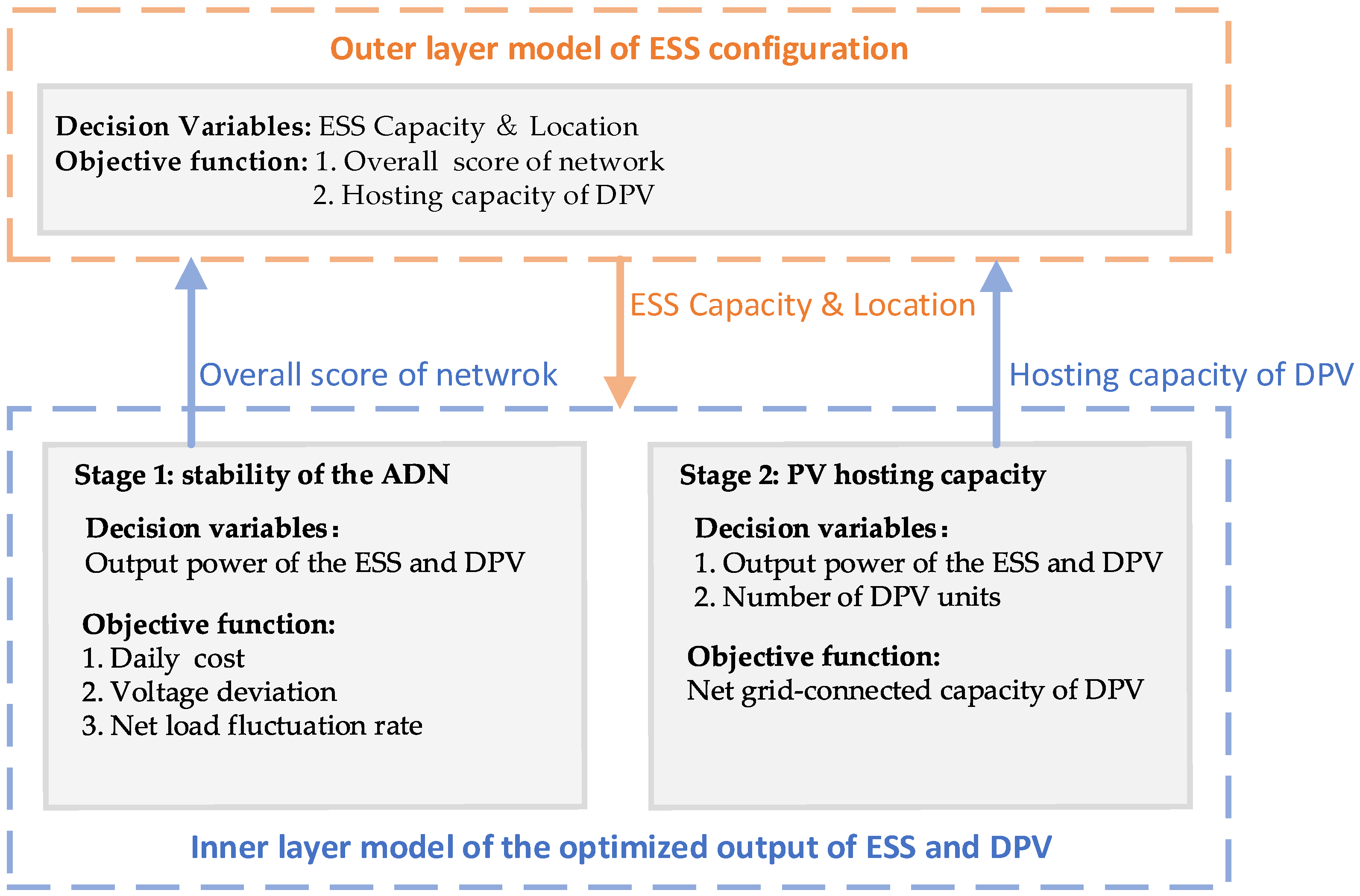
A two-layer, double-stage ESS configuration model is constructed. The outer layer is a configuration layer for the ESS position and capacity. The inner layer is the optimization operation layer, including the first stage of current network operation optimization and the second stage of further DPV hosting capacity improvement. By configuring the ESS, both the operation stability and the DPV hosting capacity are simultaneously improved.

(2)

A targeted solution strategy is designed to effectively support the configuration model. In the constructed model, single-objective, dual-objective and multi-objective optimization problems are all involved. Thus, solver and intelligent algorithms are used for the corresponding stage. To obtain a compromised optimal solution for multi-objective problems, a modified Technique for Order of Preference by Similarity to Ideal Solution (TOPSIS) and analytic hierarchy process–anti-entropy weighting method are used. The proposed solving strategy takes full advantage of the algorithms’ characteristics, which promotes solving efficiency.

(3)

Multiple cases with different operation conditions, different solving algorithms and different configuration models are analyzed and compared. The proposed method offers optimal operation and configuration results for all cases. The effectiveness has been verified.

The remainder of this paper is organized as follows. Section 2 introduces the modeling of ESSs and DPVs. The two-layer, double-stage ESS configuration model is also elaborated. Section 3 designs the solution strategy and algorithm for the proposed optimization model. Section 4 presents case studies under multiple conditions. Section 5 gives the conclusions.

2. Modeling

Firstly, key equipment modeling is introduced, including the modeling of the ESS and the DPV. Then, a two-stage, double-layer configuration model of the ESS in ADNs is proposed.

2.1. Modeling of Energy Storage System

Based on existing energy storage technologies, ESSs can be primarily categorized into mechanical storage, battery storage, chemical storage and electromagnetic storage, according to their energy storage mechanisms. This paper focuses on battery ESSs for energy storage configuration. The battery ESS model mainly considers charge and discharge power limits, state of operation constraints and capacity update restrictions.

$$\left|P_{i,t}^{\mathrm{ESS}}\right|\le P_{i,\max }^{\mathrm{ESS}},i\in N_{\mathrm{all}},t\in T$$

(1)

$$E_{i,\min }^{\mathrm{ESS}}\le E_{i,t}^{\mathrm{ESS}}\le E_{i,\max }^{\mathrm{ESS}},i\in N_{\mathrm{all}},t\in T$$

(2)

$$E_{i,t+1}^{\mathrm{ESS}}=E_{i,t}^{\mathrm{ESS}}+{\eta }_{i,t}{P}_{i,t}^{\mathrm{ESS}},i\in N_{\mathrm{all}},t\in T$$

(3)

$${\eta }_{i,t}=\left\{\begin{array}{c}{\eta }_i^c,P_{i,t}^{ESS}\ge 0\\ {\eta }_i^d,P_{i,t}^{ESS}<0\end{array}\right.$$

(4)

$$E_{i,\mathrm{T}}^{\mathrm{ESS}}=E_{i,0}^{\mathrm{ESS}},i\in N_{\mathrm{all}}$$

(5)

where $N_{\mathrm{all}}$ represents the set of ESS nodes; $P_{i,\max }^{\mathrm{ESS}}$ denotes the maximum charge and discharge power of the i-th ESS node during time period t; $E_{i,\min }^{\mathrm{ESS}}$ and $E_{i,\max }^{\mathrm{ESS}}$ are the minimum and maximum state of storage, which are set as 10% and 90% of the rated capacity, respectively; $E_{i,t}^{\mathrm{ESS}}$ represents the remaining energy of the i-th ESS node during time period t; ${\eta }_{i,t}$ is the charging and discharging efficiency of the i-th ESS node during time period t; ${\eta }_i^{\mathrm{c}}$ and ${\eta }_i^{\mathrm{d}}$ are the charging and discharging efficiencies of the ESS; and $E_{i,\mathrm{T}}^{\mathrm{ESS}}$ denotes the remaining energy at the end of a scheduling period. Equation (5) indicates that the remaining energy at the end of one scheduling period should equal the initial energy at the start of the next scheduling period to maintain consistency of the initial value.

2.2. Modeling of Distributed Photovoltaic

2.2.1. K-Means Algorithm

K-means clustering is an unsupervised learning algorithm. It partitions data into K clusters by minimizing the within-cluster sum of squares (WCSS). Each data point is assigned to the cluster with the nearest centroid using Euclidean distance, iterating until centroid convergence [24].

When processing 8760 h solar irradiance data points, K-means efficiently groups similar photovoltaic output scenarios into four typical days. These typical days represent seasonal patterns of spring, summer, autumn and winter. The algorithm proceeds through two key phases:

(1)

Cluster formation by minimizing WCSS

$$\mathrm{WCSS}={\displaystyle \sum _{i=1}^K{\displaystyle \sum _{\chi \in C_i}{‖\chi -{\mu }_i‖}^2}}$$

(6)

where K is the number of clusters; $C_i$ denotes the i-th cluster; $\chi$ represents a data point within the cluster; and ${\mu }_i$ is the centroid of $C_i$, which is the average of all data points in the i-th cluster.

(2)

Probability calculation

The occurrence probability $p_i$ for each typical day is derived from its cluster’s relative size:

$$p_i={\displaystyle \frac{\left|C_i\right|}{8760}}$$

(7)

where $\left|C_i\right|$ is the quantity of data in the i-th cluster.

2.2.2. Distributed Photovoltaic Modeling

Photovoltaic output is affected by meteorological conditions such as solar irradiance and temperature. The maximum output in a given period is the value of maximum power point tracking. To enhance stability, the upper and lower limits of photovoltaic output are set to satisfy the following:

$$(1-\gamma )P_{m,t,k}^{\mathrm{PV},\max }\le P_{m,t,k}^{\mathrm{PV}}\le P_{m,t,k}^{\mathrm{PV},\max },m\in ({\mathrm{M}}_1+{\mathrm{M}}_2)$$

(8)

where $P_{m,t,k}^{\mathrm{PV}}$ represents the actual power of DPV node m during time period t under scenario k; $P_{m,t,k}^{\mathrm{PV},\max }$ denotes the maximum power point tracking value of DPV node m during time period t under scenario k; $\gamma$ is the maximum curtailment rate; ${\mathrm{M}}_1$ is the original number of DPV nodes in the ADN; and ${\mathrm{M}}_2$ represents the number of DPV nodes that are further integrated into the ADN.

2.3. Two-Layer Double-Stage Optimization Configuration Model

Since the ESS optimization configuration problem involves numerous decision variables and constraints, it is a complex, high-dimensional, nonlinear mixed-integer problem. Thus, a two-layer, double-stage ESS optimization configuration model is proposed. The framework of the model is illustrated in Figure 1.

To simultaneously improve the current operation stability of the system and further hosting capacity of DPVs, a two-layer, double-stage ESS configuration method is proposed. The outer layer is the ESS configuration layer. The decision variables are the location and capacity of the ESS. The objective functions are the overall score of network operation and the number of DPV access units. The generated ESS configuration scheme is transmitted to the inner layer. The inner layer is the optimization operation layer. It contains the first stage of current operation optimization and the second stage of further DPV hosting capacity optimization. In the first stage, the decision variables are the output power of the ESS and DPV. The objective function is to minimize daily cost, voltage deviation and net load fluctuation rate. In the second stage, the decision variables include the quantity of DPV access units and the output power of the ESS and DPV. The objective function is the maximum hosting capacity of the DPV. The optimization results of the two stages of the inner layer are transmitted to outer layer. Comprehensive optimization is carried out in the outer layer for the optimal ESS configuration.

2.3.1. Outer-Layer Optimization Configuration Model

The objective of the outer optimization model includes two parts: the overall score of the network operation and the hosting capacity of the DPV.

The first objective function is to maximize the overall score under the first-stage operation mode, which is defined as the Euclidean distance between the final compromised solution set selected by the improved TOPSIS method and the worst solution set:

$$F_1=\max (S_{\mathrm{ADN}})=\max (\sqrt{\sum _{h=1}^{\mathrm{H}}{[f_h(x_b)-f_{h-}]}^2})$$

(9)

where $S_{\mathrm{ADN}}$ represents the overall score of the distribution network operation; $x_b$ is the final compromised solution set selected by the improved TOPSIS method; $f(x_b)$ denotes the set of the inner layer’s first-stage optimization objectives corresponding to the final compromised solution set $x_b$; H is the number of optimization objectives in the inner layer’s first stage; and $f_{-}$ represents the worst-case optimization objective set without ESS configuration.

The second objective is to maximize the DPV hosting capacity in the second-stage operation mode.

$$F_2=\max \left(\sum _{m=1}^{M_2}{S}_{\mathrm{DPV}}(m)\right)$$

(10)

where $S_{\mathrm{DPV}}(m)$ represents the allowable DPV hosting capacity at node m; and ${\mathrm{M}}_2$ represents the number of nodes where the DPV can be integrated.

2.3.2. Inner-Layer First-Stage Optimization Operation Model

The first-stage optimization operation model of the inner layer comprehensively considers operation economy and stability, selecting the daily cost, voltage deviation and net load fluctuation rate as objectives to construct the model.

(1)

Daily Cost

The daily cost of the distribution network includes the average daily investment and construction cost, operation and maintenance cost, network loss cost, cost of purchasing electricity from the upper-level grid and curtailment cost of the DPV. The objective function can be expressed as follows:

$$f_1=\min (C_{\mathrm{plan}})=\min \sum _{k=1}^{\mathrm{K}}p(k)(C_{\mathrm{inv}}+C_{\mathrm{main},}+C_{\mathrm{nl}}+C_{\mathrm{buy}}+C_{\mathrm{q}})$$

(11)

where K is the total number of clustered scenarios; $p(k)$ represents the probability of scenario k; and $C_{\mathrm{plan}}$, $C_{\mathrm{inv}}$, $C_{\mathrm{main}}$, $C_{\mathrm{nl}}$, $C_{\mathrm{buy}}$ and $C_{\mathrm{q}}$ are the daily total planed cost, daily average investment and construction cost, operation and maintenance cost, network loss cost, cost of purchasing electricity from the upper-level grid and curtailment cost, respectively.

$$C_{\mathrm{inv}} ={\displaystyle \frac{1}{365}}{\displaystyle \frac{{\mathrm{r}}^{\mathrm{ESS}}{(1+{\mathrm{r}}^{\mathrm{ESS}})}^{{\mathrm{y}}^{\mathrm{ESS}}}}{{(1+{\mathrm{r}}^{\mathrm{ESS}})}^{y^{\mathrm{ESS}}}-1}}[{\mathrm{C}}_{\mathrm{E},\mathrm{inv}}^{\mathrm{ESS}}{E}_{\mathrm{inv}}^{\mathrm{ESS}}+{\mathrm{C}}_{\mathrm{P},\mathrm{inv}}^{\mathrm{ESS}}{P}_{\mathrm{inv}}^{\mathrm{ESS}}]$$

(12)

where ${\mathrm{r}}^{\mathrm{ESS}}$ represents the discount rate of the ESS; ${\mathrm{y}}^{\mathrm{ESS}}$ denotes the service life of the ESS; and ${\mathrm{C}}_{\mathrm{E},inv}^{\mathrm{ESS}}$ and ${\mathrm{C}}_{\mathrm{P},\mathrm{inv}}^{\mathrm{ESS}}$ are the unit capacity investment cost and unit power investment cost of the ESS, respectively.

$$C_{\mathrm{main}}=\sum _{t=1}^{\mathrm{T}}(\sum _{i=1}^{\mathrm{B}}{\mathrm{C}}_{\mathrm{ESS}}\left|P_{i,t}^{\mathrm{ESS}}\right|+\sum _{m=1}^{{\mathrm{M}}_1}{\mathrm{C}}_{\mathrm{PV}}{P}_{m,t}^{\mathrm{PV}})$$

(13)

$$C_{\mathrm{nl}}={\zeta }_{\mathrm{nl}}^{\mathrm{PV}}\sum _{t=1}^T{P}_t^{\mathrm{loss}}$$

(14)

where B represents the number of ESS nodes; M₁ denotes the original number of DPV nodes in the ADN; ${\mathrm{C}}_{\mathrm{PV}}$ and ${\mathrm{C}}_{\mathrm{ESS}}$ are the operation and maintenance costs per unit of photovoltaic power and ESS charge/discharge power, respectively; ${\zeta }_{\mathrm{nl}}^{\mathrm{PV}}$ is the price per unit of network loss; and $P_{\mathrm{loss},t}$ represents the line losses of the system during time period t.

$$C_{\mathrm{buy}}=\sum _{t=1}^{\mathrm{T}}{C}_t^{\mathrm{buy}}{P}_t^{\mathrm{buy}}$$

(15)

$C_t^{\mathrm{buy}}$ represents the time-of-use electricity price; and $P_t^{\mathrm{buy}}$ denotes the purchased power between the ADN and the upper-level grid during time period t.

$$C_{\mathrm{q}}=C_{\mathrm{q}}^{\mathrm{PV}}\sum _{m=1}^{{\mathrm{M}}_1}\sum _{t=1}^{\mathrm{T}}(P_{m,t}^{\mathrm{PV},\max }-P_{m,t}^{\mathrm{PV}})$$

(16)

where $C_{\mathrm{q}}^{\mathrm{PV}}$ represents the penalty price per unit of curtailed power; $P_{m,t}^{\mathrm{PV},\max }$ denotes the maximum power point tracking value of the DPV at node m during time period t; and $P_{m,t}^{\mathrm{PV}}$ represents the actual power of the DPV at node m during time period t.

(2)

Voltage Deviation

The integration of the DPV can exacerbate voltage fluctuations. Voltage deviation $U_{VD}$ is used to evaluate the extent of voltage fluctuations.

$$f_2=\min (U_{\mathrm{VD}})=\min \sum _{k=1}^{\mathrm{K}}p(k)\left(\sum _{t=1}^{\mathrm{T}}\sum _{n=1}^{\mathrm{N}}|U_{n,t}-{\overline{U}}_n|\right)$$

(17)

where ${\overline{U}}_n$ represents the average voltage of node n over the scheduling period; $U_{n,t}$ denotes the voltage value of node n during time period t; and N is the total number of nodes.

(3)

Net Load Fluctuation Rate

Net load is defined as the residual system load not served by renewable energy generation. Following the integration of the DPV, due to its inherent output variability and reverse load characteristics, substantial net load fluctuations and peak-to-valley differences can occur, posing a risk to power balance. The configuration of flexible resources for regulation can mitigate the loading rate of the lines. Consequently, the fluctuation of the net load curve serves as a critical indicator of the power system’s flexibility and reliability. The Coefficient of Variation (CV), a statistical metric for assessing relative dispersion, is employed to quantify the net load fluctuation rate.

$$f_3=\min (\mathrm{CV})=\min \sum _{k=1}^{\mathrm{K}}p(k)\left({\displaystyle \frac{\sqrt{\frac{1}{\mathrm{T}}{\displaystyle \sum _{t=1}^{\mathrm{T}}}{(P_{\mathrm{C}}(t)-{\overline{P}}_{\mathrm{C}})}^2}}{{\overline{P}}_{\mathrm{C}}}}\right)\times 100\%$$

(18)

where $P_{\mathrm{C}}(t)$ represents the net load of the system during time period t; and ${\overline{P}}_{\mathrm{C}}$ denotes the average net load.

2.3.3. Inner-Layer Second-Stage Hosting Capacity Optimization Model

The integration of DPVs into ADNs will change network loss. Thus, the evaluation of DPV hosting capacity considers both the grid-connected capacity of distributed DPVs and the network loss caused by DPV integration. The equivalent grid-connected DPV capacity is defined as the difference between these two factors, and its maximum value represents the DPV hosting capacity of the ADN. Thus, the second-stage objective function is as follows.

$$f_4=\max (\sum _{m=1}^{{\mathrm{M}}_1+{\mathrm{M}}_2}{P}^{\mathrm{DPV}}(m)-P^{\mathrm{loss}})$$

(19)

where $P^{\mathrm{DPV}}(m)$ represents the total power output of the DPV at node m over the operating period; and $P^{\mathrm{loss}}$ denotes the total line losses.

2.4. Constraints

(1)

Power flow constraints

The following constraints must be satisfied in power flow calculations.

$$\left\{\begin{array}{l}{P}_a=U_a{\displaystyle \sum _{n=1}^{\mathrm{N}}}{U}_b\left(G_{ab}\cos {\theta }_{ab}+B_{ab}\sin {\theta }_{ab}\right)\\ Q_a=U_a{\displaystyle \sum _{n=1}^{\mathrm{N}}}{U}_b\left(G_{ab}\sin {\theta }_{ab}-B_{ab}\cos {\theta }_{ab}\right)\end{array}\right.$$

(20)

where $P_a$ and $Q_a$ represent the active power and reactive power at node a, respectively; $U_a$ and $U_b$ denote the voltages at nodes a and b, respectively; N is the total number of nodes; $G_{ab}$ and $B_{ab}$ are the conductance and susceptance of the line between node a and b, respectively; and ${\theta }_{ab}$ is the phase angle difference between nodes a and b.

The active power output and reactive power output from all types of generators must equal the active load demand and the reactive load demand plus the active and reactive power losses in the system.

$$\left\{\begin{array}{c}{P}_{a,t}^{\mathrm{buy}}+P_{a,t}^{\mathrm{PV}}+P_{a,t}^{\mathrm{ESS}}=P_{a,t}^{\mathrm{Load}}+P_{a,t}^{\mathrm{loss}}\\ Q_{a,t}^{\mathrm{buy}}=Q_{a,t}^{\mathrm{Load}}+Q_{a,t}^{\mathrm{loss}}\end{array}\right.$$

(21)

where $P_{a,t}^{\mathrm{buy}}$, $P_{a,t}^{\mathrm{PV}}$ and $P_{a,t}^{\mathrm{ESS}}$ are the main grid power, PV power and ESS active power of node a, respectively; $P_{a,t}^{\mathrm{Load}}$ and $P_{a,t}^{\mathrm{loss}}$ represent the active load and line losses of node a, respectively; $Q_{a,t}^{\mathrm{buy}}$ is the main grid power and PV reactive power of node a, respectively; and $Q_{a,t}^{\mathrm{Load}}$ and $Q_{a,t}^{\mathrm{loss}}$ represent the reactive load and line losses of node a, respectively.

(2)

Nodal Voltage Constraints

$$U_{\min }\le U_n\le U_{\max }$$

(22)

where $U_{\min }$ and $U_{\max }$ represent the lower and upper limits of the node voltage, respectively.

(3)

Node selection constraints for ESS configuration

$$N\subseteq N_{\mathrm{all}}$$

(23)

where N is the set of nodes approved for ESS configuration; and $N_{\mathrm{all}}$ contains all technically feasible candidate nodes for ESS configuration.

(4)

Node selection constraints for DPV integration

$$M_2\subseteq M_{\mathrm{all}}$$

(24)

where $M_2$ represent is the set of nodes approved for DPV integration; and $M_{\mathrm{all}}$ contains all technically feasible candidate nodes for DPV integration.

(5)

Capacity constraints for ESS configuration

$$0\le E^{\mathrm{ESS}}\le E_{\max }^{\mathrm{ESS}}$$

(25)

where $E^{\mathrm{ESS}}$ denotes the deployed ESS capacity; and $E_{\max }^{\mathrm{ESS}}$ represents the maximum permissible ESS capacity.

(6)

Capacity constraints for DPV integration

$$0\le E^{\mathrm{DPV}}\le E_{\max }^{\mathrm{DPV}}$$

(26)

where $E^{\mathrm{DPV}}$ denotes the deployed DPV capacity; and $E_{\max }^{\mathrm{DPV}}$ represents the maximum permissible DPV capacity.

(7)

Reverse load rate constraints

According to the Guidelines for Evaluating the Hosting Capacity of Distributed Power Integration into the Grid (DL/T 2041) [25], if the reverse load rate $\lambda$ > 80%, the integration of new distributed power projects should be suspended until the grid’s hosting capacity is effectively improved. The reverse load rate $\lambda$ is calculated as follows:

$$\lambda ={\displaystyle \frac{P_{\mathrm{D}}-P_{\mathrm{L}}}{S_{\mathrm{e}}}}\times 100\%$$

(27)

where $P_{\mathrm{D}}$ represents the output of the distributed power source; $P_{\mathrm{L}}$ denotes the equivalent load during the same period, which is the load minus the output of other power sources besides the distributed power; and $S_{\mathrm{e}}$ represents the actual operational limit of the transformer or line.

(8)

ESS operational constraints

The SOC of the ESS, along with its operational charging and discharging power and capacity constraints, can be described by Equations (1)–(5).

3. Solution Strategy and Algorithm

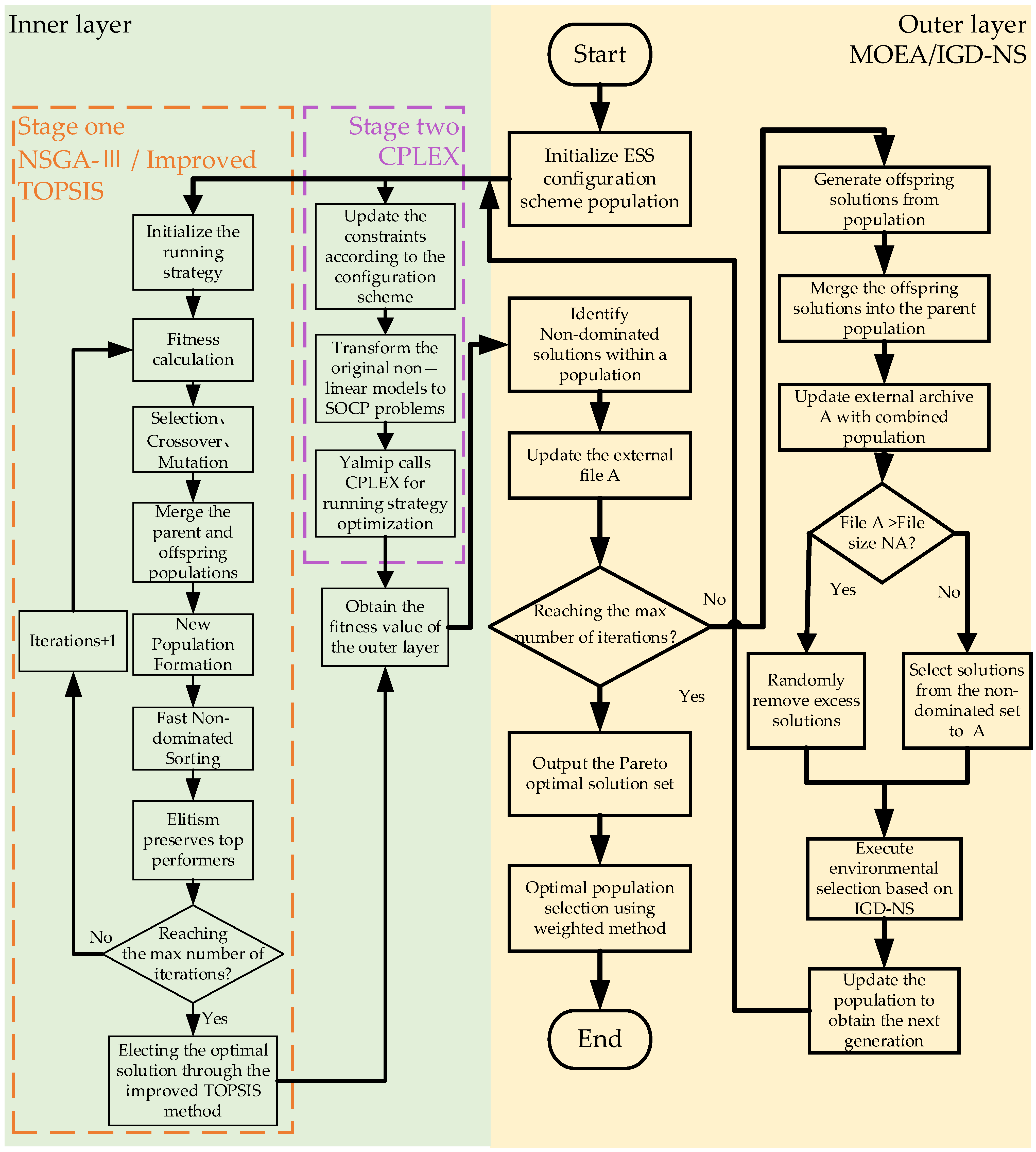
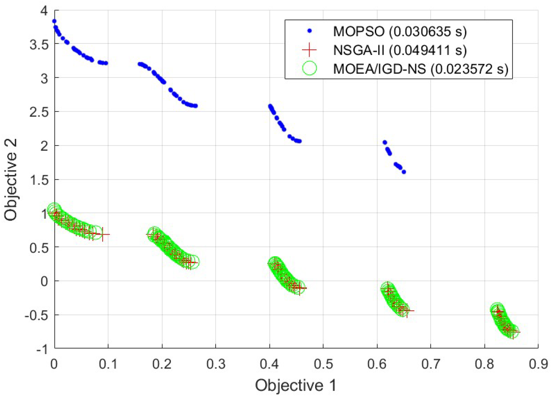
The proposed two-layer, double-stage ESS optimization configuration model requires several different solving processes, including single-objective optimization, multi-objective optimization and nested solving of both inner and outer layers. To improve solving efficiency, different solving methods are employed for different optimization problems. Specifically, Multi-Objective Evolutionary Algorithm based on Improved Inverted Generational Distance and Non-dominated Sorting (MOEA/IGD-NS), Non-dominated Sorting Genetic Algorithm-III (NSGA-III) and CPLEX solver are used to solve the respective optimization problems. The detailed workflow of this process is illustrated in Figure 2.

3.1. Solution Strategy for the Outer-Layer Model

The MOEA/IGD-NS is employed for solving the outer-layer model. The algorithm, inspired by biological evolution and population genetics mechanisms in nature, is renowned for its simplicity, minimal control parameters and outstanding optimization performance [26]. The MOEA/IGD-NS introduces an enhanced IGD-NS to evaluate the convergence and diversity of the solution set. It identifies and removes non-contributing solutions. Only solutions that effectively contribute to the optimization objectives are retained in the solution set. Thus, it is suitable for addressing the two-stage ESS configuration problem in a comprehensive manner. The flowchart of the MOEA/IGD-NS applied for outer-layer optimization is illustrated in Figure 2, which depicts the outer-layer ESS planning process.

Specific process introduction:

1. The values of the non-dominated solutions are passed from the inner layer.

2. Establish external archive A to store a set of the best non-dominated solutions discovered so far, as a reference set for IGD-NS calculations.

3. Update external archive A and repeat the evolutionary process until the termination condition is met.

4. Identify non-contributing solutions within the IGD-NS metric.

5. Eliminate the solutions that have the smallest contribution to the IGD-NS metric value.

6. Update the population and return to the inner layer to obtain the non-dominated solution.

7. Continue the iterative evolutionary process until the termination criteria are satisfied.

3.2. Solution Strategy for the Inner-Layer Model

The inner layer holds a two-stage optimization framework. The optimization of the first stage is a tri-objective optimization problem. It is solved by NSGA-III algorithm. The Pareto optimal solution is determined through an enhanced decision-making approach combining TOPSIS with the analytic hierarchy process (AHP)–anti–entropy weighting Method. The second stage focuses on DPV hosting capacity optimization. The objective function is the maximal equivalent grid-connected DPV capacity. It is solved by CPLEX optimizer. Figure 2 illustrates the complete solution workflow, detailing the interaction between two stages.

3.2.1. Solution Strategy of the First Stage

NSGA-III is an evolutionary algorithm designed to solve multi-objective optimization problems [27]. NSGA-III begins with non-dominated sorting of the individuals in the population, assigning each individual to a specific non-dominated rank. Then, a set of predefined reference points is used to guide the searching process. Finally, a niche-preservation operation is employed to select individuals, ensuring that the population covers different regions of the Pareto front. In this study, NSGA-III is used to optimize the output power of the DPV and ESS in the inner layer. NSGA-III yields a set of Pareto optimal solutions. To obtain the compromised optimal solution, an enhanced TOPSIS method incorporating subjective and objective weightings is employed.

(1)

TOPSIS-based Pareto Solution Selection

The TOPSIS method makes decisions by calculating the distances between the alternatives and the positive ideal solution or negative ideal solution, respectively. The selected solution is the one that has the minimum distance to the positive ideal solution and the maximum distance to the negative ideal solution, thereby obtaining the final compromised optimal solution [28].

To ensure comparability across objective functions with heterogeneous dimensions, normalization is performed as follows.

$$f_m^{\prime }(x_i)={\displaystyle \frac{f_m(x_i)-\min (f_m)}{\max (f_m)-\min (f_m)}}\hspace{1em}m=1,2,3$$

(28)

where $x_i$ represents the i-th set of optimization objectives, encompassing all $P^{\mathrm{DPV}}$ and $P^{\mathrm{ESS}}$; the upper bound max(f_m) denotes the negative ideal solution of the m-th objective function, corresponding to the optimization result obtained without ESS deployment; and min(f_m) represents the ideal minimum value as 0, corresponding to the theoretically optimal solution.

The TOPSIS method selects the compromised optimal solution from the Pareto front by maximizing the optimal fit degree $d(x_i)$ and quantifying the solution’s proximity to the positive ideal solution while maximizing its distance from the negative ideal solution. The formula is given as follows:

$$d(x_i)={\displaystyle \frac{d_{-}(x_i)}{d_{+}(x_i)+d_{-}(x_i)}}$$

(29)

$$d_{+}(x_i)=\sqrt{\sum _{m=1}^3{[W_m{f}_m^{\prime }(x_i)-W_m{f}_{m+}^{\prime }]}^2}$$

(30)

$$d_{-}(x_i)=\sqrt{\sum _{m=1}^3{[W_m{f}_m^{\prime }(x_i)-W_m{f}_{m-}^{\prime }]}^2}$$

(31)

$$f_{\pm }^{\prime }=[f_{1\pm }^{\prime },f_{2\pm }^{\prime },f_{3\pm }^{\prime }]$$

(32)

where $d_{+}(x_i)$ and $d_{-}(x_i)$ represent the distances from solution $x_i$ to the positive ideal solution or the negative ideal solution, respectively. After normalization, the positive ideal solution is the point $f_{+}^{\prime }$ (0,0,0), and the negative ideal solution is the point $f_{-}^{\prime }$ (1,1,1). $W_m$ represents the weight corresponding to the optimization objective $f_m$, $0<W_m<1$, and ${\displaystyle \sum _{m=1}^3}{W}_m=1$.

(2)

Combined Weighting: AHP and Anti-Entropy Method

To ensure reliable TOPSIS evaluation results, a combined weighting approach is used by integrating subjective AHP weights with objective entropy weights. Thus, expert judgment and objectivity can be balanced.

Based on the established indicator system, a three-indicator AHP is used to determine the subjective weights of each indicator. The specific algorithm steps are as follows [29].

Based on expert opinions, the importance of each indicator is compared pairwise to form a judgment matrix A, which is as follows:

$$A=\left[\begin{array}{ccc}1& a_{12}& a_{13}\\ 1/a_{12}& 1& a_{23}\\ 1/a_{13}& 1/a_{23}& 1\end{array}\right]$$

(33)

where $a_{ij}$ represents the importance of objective i relative to objective j, with values ranging from [1, 9]. The values indicate the level of importance, ranging from “equally important” to “extremely more important” for the former objective compared to the latter.

To avoid significant discrepancies between subjective judgment and objective reality, a consistency check is performed on the judgment matrix by calculating the consistency ratio (CR) value, which is calculated as follows:

$$CI={\displaystyle \frac{{\lambda }_{\max }-3}{3-1}}$$

(34)

$$CR=CI/RI$$

(35)

where ${\lambda }_{\max }$ is the maximum eigenvalue of the judgment matrix. CI represents consistency indicators; RI is the Random Consistency Index.

If the CR value is less than 0.1, the consistency of the judgment matrix is acceptable. The normalized eigenvector of the judgment matrix is then used as the weight vector to obtain the subjective weights for each indicator, denoted as $w={[w_1,w_2,w_3]}^{\mathrm{T}}$.

$$w_j(x_i)={\displaystyle \frac{v_j(x_i)}{{\displaystyle {\sum }_{j=1}^3{v}_j}(x_i)}},j=1,2,3$$

(36)

where $v_j$ represents the component corresponding to the j-th indicator in the initial feature vector.

A low-sensitivity anti-entropy weighting approach is employed for objective indicator weighting. The anti-entropy weight formula is calculated as follows:

$$e_j(x_i)=1+{\displaystyle \frac{1}{\ln 3}}\sum _{j=1}^3{f}_j^{\prime }(x_i)\cdot \ln f_j^{\prime }(x_i)$$

(37)

In the formula, $e_j(x_i)$ represents the inverse entropy of the j-th indicator of solution $x_i$.

After the normalization of anti-entropy, the final calculation for obtaining the objective weights $w^{\prime }={[w_1^{\prime },w_2^{\prime },w_3^{\prime }]}^{\mathrm{T}}$ is calculated as follows:

$$w_j^{\prime }(x_i)=e_j(x_i)/\sum _{j=1}^3{e}_j(x_i),j=1,2,3$$

(38)

The comprehensive weight calculation is as follows, which is obtained by combining the subjective and objective weights.

$$W(x_i)=\alpha w(x_i)+(1-\alpha )w^{\prime }(x_i),\alpha =0.5$$

(39)

Take the comprehensive weight results into Equations (30) and (31) to calculate the optimal fit of each candidate objective set. After ranking, the solution with the highest fit is selected as the final compromised solution.

3.2.2. Solution Strategy of the Second Stage

In the second stage of the inner layer, optimization is a single-objective problem. The CPLEX solver is used for solving the problem. In the power flow model, there are nonlinear terms such as complex power flow $V_i{I}_{ij}^{*}$ and active power $r_{ij}|I_{ij}{|}^2$. This causes the optimal power flow model to be non-convex, making it difficult for solvers to solve directly. To facilitate rapid solving, the paper adopts a second-order cone relaxation method to convexify the above model, converting the non-convex model into a convex model [30].

4. Case Study

To demonstrate the validity of the proposed two-layer configuration model of the ESS, a case study is performed on a modified IEEE 33 bus active distribution network model, as depicted in Figure 3. In the ADN, two DPVs are connected at node 7 and node 16. Nodes 5–19 and 25–27 are the optional sites for ESS configuration in the outer layer. Node 8 and node 29 are the optional locations for DPV integration in the second stage for further DPV hosting capacity evaluation. The case study objective is to configure the ESS at two different locations.

4.1. Parameter Settings

The proposed method is simulated on a modified IEEE 33-node ADN system with base voltage of 12.66 kV and base capacity of 1 MVA. The line power flow limit is set as 6 MW. Node voltage constraints are maintained between 0.93 pu and 1.07 pu to ensure stable operation. The system load is 3715 kW + j2300 kVar. Each integrated DPV unit holds a rated capacity of 50 kW. The configured ESS units are 10 kWh/5 kW units. The maximum quantity of ESS units is 150 units per node. The initial SOC is set to 20% and an operational SOC range is set between 10 and 90%.

The subjective weighting coefficients for the multi-objective evaluation criteria are presented in

Table 1. The subjective weight of indicators.

Function	${\mathit{f}}_1$	${\mathit{f}}_2$	${\mathit{f}}_3$
Subjective weight	0.7143	0.1429	0.1429

. The complete parameter settings for system components are detailed in

Table 2. Time-of-use electricity price.

Period	Electricity Price/[¥·(kW·h)−1]
Valley Period (0–8)	0.2039
Shoulder Period (9–12, 15–19, 22–24)	0.5318
Peak Period (12–14, 19–22)	0.9497

and

Table 3. Relevant parameters.

Parameters	Value
Cost of ESS Unit Capacity Investment/(¥·(kW·h)−1)	1070
Cost of ESS Unit Power Investment/(¥·(kW)−1)	1050
Cost of DPV Unit Operation and Maintenance/(¥·(kW)−1)	0.1
Cost of ESS Unit Operation and Maintenance/(¥·(kW)−1)	0.05
Cost of Curtailed DPV Energy Penalty/(¥·(kW)−1)	0.8
Network Loss Cost/(¥·(kW)−1)	0.8
Charging and Discharging Efficiency	0.9
Discount Rate/%	8
SOC Minimum Percentage%	10
SOC Maximum Percentage%	90
DPV Maximum Curtailment Rate/%	10

.

Figure 4 presents the profiles of the DPV and load. Figure 4a displays the raw annual DPV generation data with 8760 h points, which were simulated from measured solar irradiance data in a typical region of China. Figure 4b illustrates the normalized typical DPV profiles derived through the K-means algorithm and the load curve. Four distinct scenarios emerge, corresponding to seasonal variations. The probabilistic weights of each scenario are quantified in

Table 4. Probability distribution of typical days.

Scenario	Season	Probability (%)
1	Summer	32.9
2	Spring	33.4
3	Autumn	19.7
4	Winter	14.0

.

4.2. Performance of the Configuration Method

4.2.1. Performance Comparison of Optimization Strategies

Four cases are designed to verify the effectiveness of the proposed method. The benchmark case, Case 1, operates without ESS configuration. Case 2 configures the ESS by considering only the first stage of the inner layer. Case 3 configures the ESS by considering only the second stage of the inner layer. Case 4 utilizes the proposed two-layer double-stage ESS configuration method. The initial DPV penetration is set at 25%. The configuration results are shown in

Table 5. Results of ESS configuration.

Case	ESS Connection Node (Capacity)	Daily Cost/¥	Voltage Deviation	Net Load Fluctuation Rate	Overall Score of Network Operation	Quantity of DPV Access Units
Case 1	——	3.8769 × 104	5.6258	0.2538	2.7543	160
Case 2	8 (150), 12 (150)	3.8586 × 104	3.4239	0.1573	4.9514	178
Case 3	16 (150), 30 (150)	3.8667 × 104	4.0563	0.1611	4.3210	180
Case 4	14 (138), 17 (148)	3.8600 × 104	3.4844	0.1639	4.9171	179

.

As seen in Table 5, without the ESS, Case 1 shows the smallest operation score and the smallest quantity of DPV access units. Without the flexible adjustment of the ESS, the daily cost, voltage deviation and net load fluctuation rate are high, indicating a bad operation state. The hosting capacity of the DPV is also limited. By configurating the ESS in Case 2, the daily cost is reduced by 1%. The configuration cost of the ESS is compensated by peak–valley arbitrage, reduced network losses and decreased DPV curtailment expenses. The power quality is also improved with a 28% lower voltage deviation and a 35% reduced net load fluctuation rate. Thus, the overall score of network operation is increased. Though without hosting capacity optimization, the hosting capacity of the DPV is also increased, demonstrating the importance of the ESS in facilitating renewable energy integration. By configuring the ESS in Case 3, the photovoltaic hosting capacity is increased by 12.5%. Because network operation is overlooked in ESS configuration, the overall score of network operation is lower compared to Case 2. In Case 4, the two stages of network operation and DPV hosting capacity are both considered in ESS configuration. The results obtain a compromised optimal solution in the operation score and DPV hosting capacity. The validation of the proposed method is proved. The configuration capacity of the ESS does not reach the upper limit, indicating the potential for optimizations in the future.

Figure 5 shows the net load curve of the first stage in Case 4. The original load curve shows a large fluctuation rate (red line). With optimal operation, the ESS and DPV are synergistically operated. During daytime, the DPV outputs active power close to MPPT. During the periods of 22:00–24:00 and 0:00–6:00, the ESS is charging in the light loading period. During the periods of 10:00–11:00 and 13:00–15:00, the ESS is also charging to consume the active power of the DPV. During the period of 17:00–22:00, the ESS discharges to balance the heavy load. Thus, the fluctuation range of net load is obviously decreased. The maximum loading rate is lowered below 50%. The optimization of network operation also improves the voltage quality. The minimum voltage distribution of nodes is shown in Figure 6. It can be seen that the voltage stays above the minimum voltage limit after ESS configuration. The voltage deviation is obviously improved.

Figure 7 shows the state of charge curves and power curves of the ESS. Both configured ESS units exhibit similar charging/discharging patterns. Charging happens during low-price/light-load periods and discharging happens during high-price/heavy-load periods, improving both stability and economic performance.

In the second stage, on the basis of ESS configuration, the DPV is further configured for the evaluation of hosting capacity. As shown in Figure 8, the net load curves reveal system constraints from node voltage limits and reverse power flow during peak generation periods. When DPV output exceeds local demand, ESSs play a crucial role in absorbing the surplus generation.

The ESSs exhibit distinct operational patterns in this stage compared to the first stage. As detailed in Figure 9, both units maintain consistent charging and discharging behaviors, with charging operations concentrated during midday hours from 12:00 to 15:00 to absorb surplus DPV generation. Discharge cycles occur during evening and overnight periods from 20:00 to 24:00 and 0:00 to 6:00 to meet nighttime load requirements. This operational strategy effectively addresses multiple technical challenges by reducing photovoltaic curtailment, minimizing network losses and controlling reverse power flow.

4.2.2. Performance Comparison of Solving Algorithms

The superiority of the MOEA/IGD-NS in solving the outer-layer configuration model is verified and compared in Figure 10. The Pareto front calculated using the MOEA/IGD-NS is much better than that calculated using MOPSO on the ZDT3 benchmark problem [31]. Though the Pareto front calculated using the MOEA/IGD-NS is comparable to that calculated using NSGA-II, the computational time of the MOEA/IGD-NS is the shortest. Thus, the superior efficiency and effectiveness of the MOEA/IGD-NS are demonstrated in two-objective optimization problems.

To prove the performance of NSGA-III in solving the first-stage inner-layer optimization model, a comparative analysis was conducted on the compromised optimal solutions obtained with NSGA-III, NSGA-II, Multi-Objective Ant Colony Optimization (MOACO) and the Multi-Objective Genetic Algorithm (MOGA). As shown in

Table 6. Comparison of optimization results solving by different algorithms.

Algorithm	Daily Cost/¥	Voltage Deviation	Net Load Fluctuation Rate	Overall Score of Network Operation
NSGA-III	3.8600 × 104	3.4844	0.1639	4.9171
NSGA-II	3.8598 × 104	3.5120	0.1632	4.9115
MOACO	3.8705 × 104	3.8923	0.1718	4.6230
MOGA	3.8652 × 104	4.2106	0.1604	4.7057

, with identical population sizes and iteration settings, NSGA-III demonstrated superior convergence performance compared to MOACO and the MOGA, while maintaining comparable effectiveness with NSGA-II. Considering the potential inclusion of additional optimization objectives in subsequent research, NSGA-III was ultimately selected as the optimization algorithm for this stage.

4.3. Other Scenario Configuration Results

To validate the proposed ESS configuration method across different DPV penetration levels, three distinct penetration levels were selected: 25%, 50% and 75%. Figure 11 presents a comparison with the benchmark case without ESS, and

Table 7. Results for different DPV penetration rates.

Penetration Rate	ESS Connection Node (Capacity)	Daily Cost/¥	Voltage Deviation	Net Load Fluctuation Rate	Overall Score of Network	Number of DPV Units
Penetration rate 25%	14 (138), 17 (148)	3.8600 × 104	3.4844	0.1639	4.9171	179
Penetration rate 50%	13 (139), 16 (100)	3.6104 × 104	4.9886	0.2339	3.4228	156
Penetration rate 75%	10 (142), 26 (117)	3.3629 × 104	6.8559	0.3327	1.7145	138

provides the ESS configuration parameters and performance indicators for each penetration level.

Figure 11 details the effectiveness of the proposed ESS configuration method across all tested DPV penetration levels. The results show that the ESS enhances the overall score of the network and increases DPV hosting capacity without additional expenditures. It also maintains sufficient capacity margins for future ADN upgrades.

Comparative analysis in Table 7 reveals that higher DPV penetration degrades operational performance and reduces hosting capacity. This is due to constrained DPV allocation nodes and ESS configuration limits. Specifically, DPV installation is restricted to nodes 8 and 29. Broader node accessibility could improve these outcomes.

To further validate the method’s adaptability, additional case studies were conducted with modified ESS constraints. The new configuration allows three ESS units, each with a 200-unit limit. As shown in

Table 8. Results for ESS configured at three nodes.

	ESS Connection Node (Capacity)	Daily Cost/¥	Voltage Deviation	Net Load Fluctuation Rate	Overall Score of Network	Number of DPV Units
Without ESS	——	3.8769 × 104	5.6258	0.2538	2.7543	160
ESS configured at three nodes	6 (176), 9 (160), 12 (196)	3.8735 × 104	2.9175	0.1084	5.5479	190

, the ESS investment cost is fully recoverable through operational benefits. The system exhibits significant improvements: voltage deviation decreases from 5.6258 to 2.9175, net load fluctuation drops from 25.38% to 10.84%, and the network operation score doubles. Additionally, DPV hosting capacity increases from 160 to 190 units.

These results confirm the method’s versatility across different scenarios through parameter adjustment. The proposed approach effectively balances ADN stability with DPV hosting capacity enhancement.

5. Conclusions

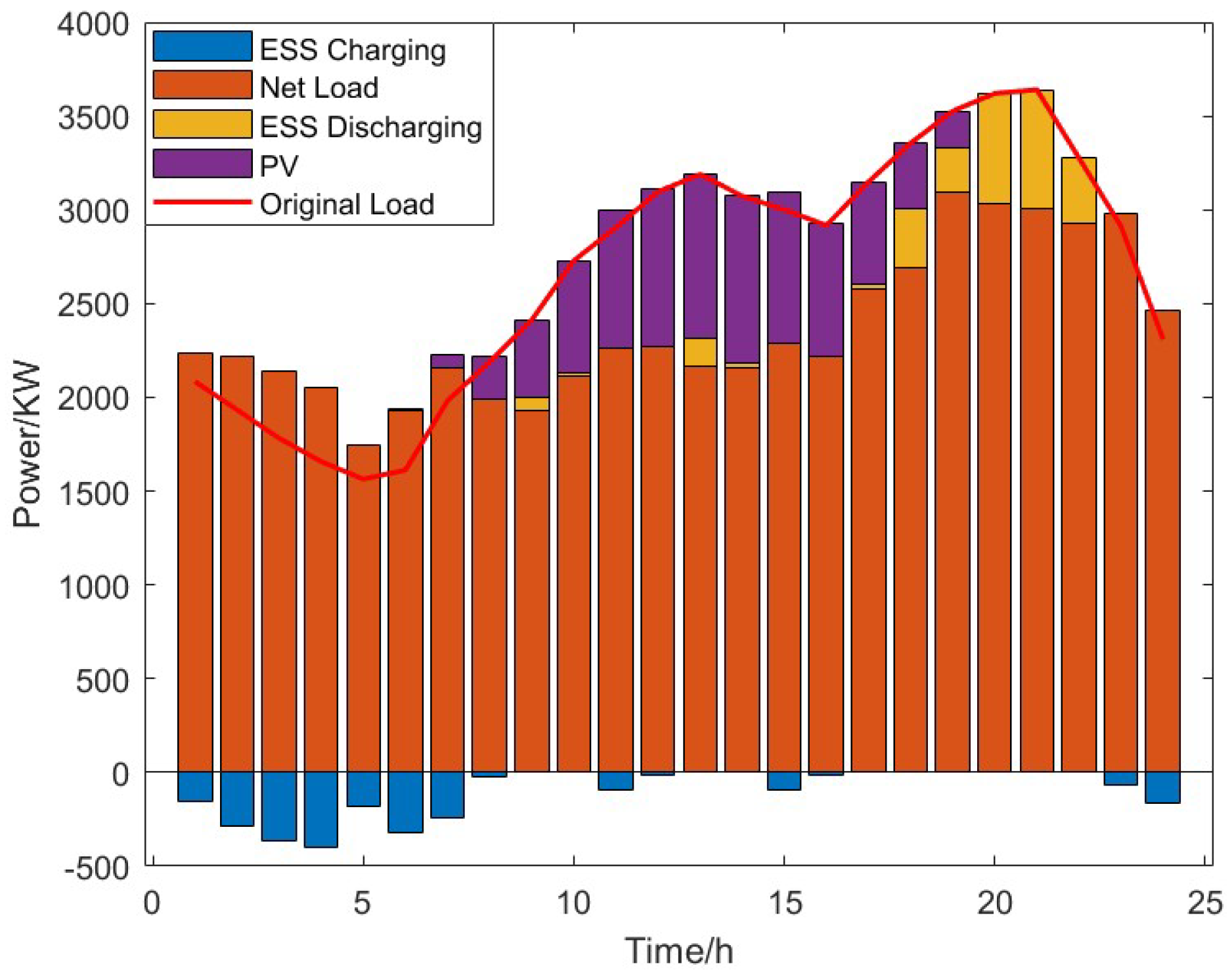
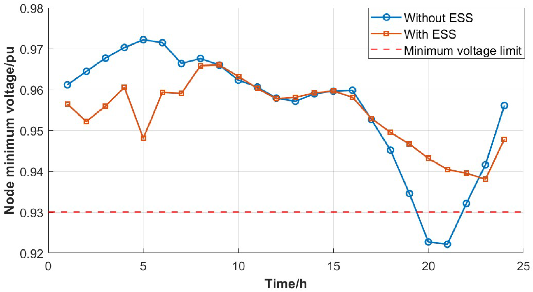
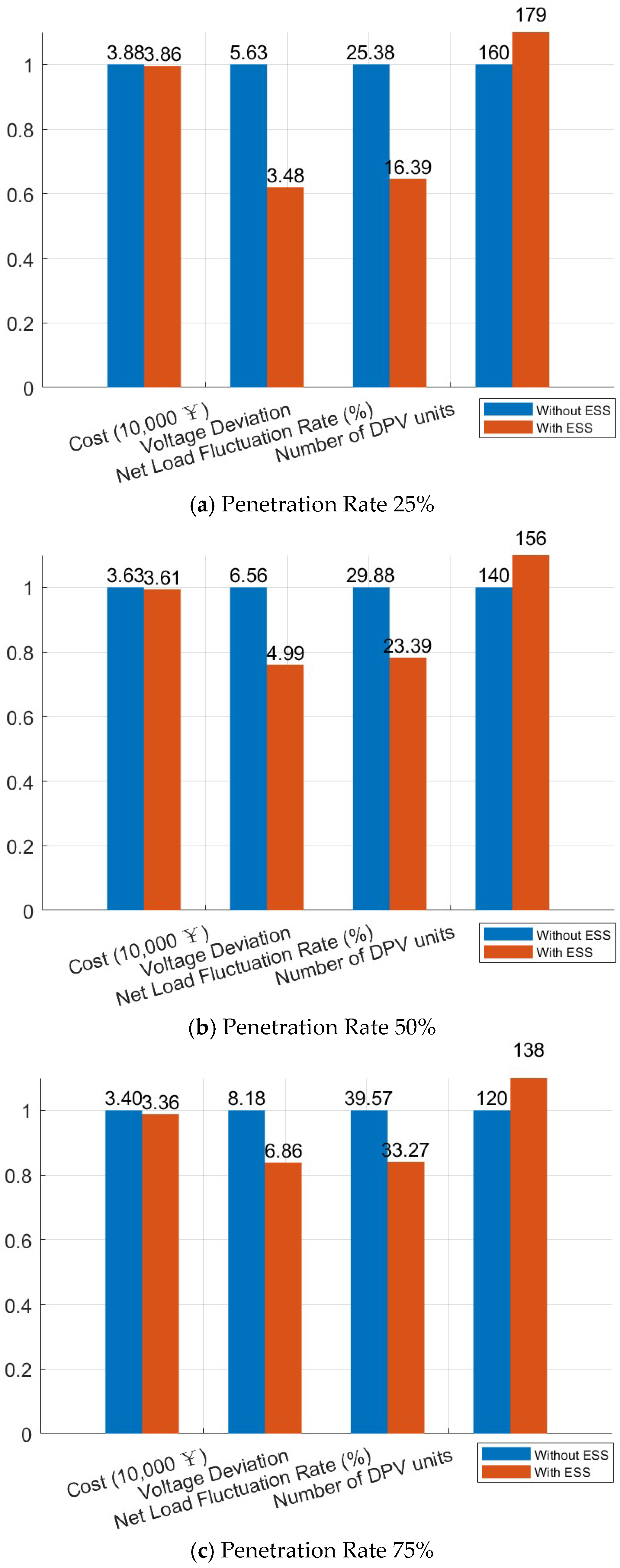
Owing to the rapid development of renewable energy, more DPVs are being injected into distribution networks. DPV hosting capacity and the stable operation of distribution networks are issues of broad concern. ESSs hold flexible charging and discharging characteristics, which provide an effective means for solving these problems. Thus, a two-layer, double-stage ESS configuration method was proposed. An ESS configuration model was constructed with two layers and two stages. The outer layer is a configuration layer for the ESS position and capacity. The two stages of the inner layer include the current network operation optimization stage and the hosting capacity improvement stage. Solving strategies and algorithms were well designed according to the characteristics of different layers and stages. Simulations were conducted and the effectiveness of the proposed method was verified. By optimizing the ESS configuration, the cost, voltage deviation and net load fluctuation rate were all reduced, improving the operation performance of the distribution network. In addition, the hosting capacity of the DPV increased by nearly 12%.

Overall, the proposed two-layer, double-stage ESS configuration method demonstrates significant advantages in improving operation stability and DPV hosting capacity, providing a potential solution for large-scale DPV integration in the future. In the following study, uncertainty modeling of DPVs, practical concerns in ESS installation and operation, and a comprehensive evaluation of hosting capacity will be focused on for the practical engineering applications of the proposed method.

References

1. Gajdzik, B.; Wolniak, R.; Nagaj, R.; Žuromskaitė-Nagaj, B.; Grebski, W.W. The Influence of the Global Energy Crisis on Energy Efficiency: A Comprehensive Analysis. Energies 2024, 17, 947. [Google Scholar] [CrossRef]
2. Shan, R.; Kittner, N. Allocation of Policy Resources for Energy Storage Development Considering the Inflation Reduction Act. Energy Policy 2024, 184, 113861. [Google Scholar] [CrossRef]
3. Zhu, H.; Cao, S.; Su, Z.; Zhuang, Y. China’s future energy vision: Multi-scenario simulation based on energy consumption structure under dual carbon targets. Energy 2024, 301, 0360–5442. [Google Scholar] [CrossRef]
4. Huang, N.; Zhao, X.; Guo, Y.; Cai, G.; Wang, R. Distribution network expansion planning considering a distributed hydrogen-thermal storage system based on photovoltaic development of the Whole County of China. Energy 2023, 278, 127761. [Google Scholar] [CrossRef]
5. Li, G.; Xie, S.; Wang, B.; Xin, J.; Li, Y.; Du, S. Photovoltaic power forecasting with a hybrid deep learning approach. IEEE Access 2020, 8, 175871–175880. [Google Scholar] [CrossRef]
6. Akram, U.; Nadarajah, M.; Shah, R.; Milano, F. A review on rapid responsive energy storage technologies for frequency regulation in modern power systems. Renew. Sustain. Energy Rev. 2020, 120, 109626. [Google Scholar] [CrossRef]
7. Li, J.; Xue, Y.; Tian, L.; Yuan, X. Research on optimal configuration strategy of energy storage capacity in grid-connected microgrid. Prot. Control Mod. Power Syst. 2017, 2, 35. [Google Scholar] [CrossRef]
8. Xie, X.; Ma, J.; Liu, W.; Zhao, W.; Xu, P.; Li, H. Functions of energy storage in renewable energy dominated power systems: Review and prospect. Proc. CSEE 2023, 43, 158–169. [Google Scholar] [CrossRef]
9. Yan, Q.; Zhang, B.; Kezunovic, M. Optimized operational cost reduction for an EV charging station integrated with battery energy storage and PV generation. IEEE Trans. Smart Grid 2019, 10, 2096–2106. [Google Scholar] [CrossRef]
10. Liao, J.; Lin, J.; Wu, G. Two-layer optimization configuration method for distributed photovoltaic and energy storage systems based on IDEC-K clustering. Energy Rev. 2024, 11, 5172–5188. [Google Scholar] [CrossRef]
11. Rawa, M.; Al-Turki, Y.; Sedraoui, K.; Dadfar, S.; Khaki, M. Optimal operation and stochastic scheduling of renewable energy of a microgrid with optimal sizing of battery energy storage considering cost reduction. J. Energy Storage 2023, 59, 106475. [Google Scholar] [CrossRef]
12. Cho, K.H.; Kim, J.; Byeon, G.; Son, W. Optimal Sizing Strategy and Economic Analysis of PV-ESS for Demand Side Management. J. Electr. Eng. Technol. 2024, 19, 2859–2874. [Google Scholar] [CrossRef]
13. Zhang, Z.; Lei, D.; Jiang, C.; Luo, J.; Xu, Y.; Li, J. A Bi-level planning model and its solution method of AC/DC hybrid distribution network based on second-order cone programming and NNC Method. Proc. CSEE 2023, 43, 70–84. [Google Scholar] [CrossRef]
14. Zhao, J.; Wang, W.; Guo, C. Hierarchical optimal configuration of multi-energy microgrids system considering energy management in electricity market environment. Int. J. Electr. Power Energy Syst. 2023, 144, 108572. [Google Scholar] [CrossRef]
15. Zhou, S.; Han, Y.; Chen, S.; Yang, P.; Mahmoud, K.; Darwish, M.M.F.; Lehtonen, M.; Zalhaf, A.S. A multiple uncertainty-based Bi-level expansion planning paradigm for distribution networks complying with energy storage system functionalities. Energy 2023, 275, 127511. [Google Scholar] [CrossRef]
16. Picioroaga, I.; Luca, M.; Tudose, A.; Sidea, D.; Eremia, M.; Bulac, C. Resilience-Driven Optimal Sizing of Energy Storage Systems in Remote Microgrids. Sustainability 2023, 15, 16002. [Google Scholar] [CrossRef]
17. Rasool, M.H.; Taylan, O.; Perwez, U.; Batunlu, C. Comparative assessment of multi-objective optimization of hybrid energy storage system considering grid balancing. Renew. Energy 2023, 216, 119107. [Google Scholar] [CrossRef]
18. Koirala, A.; Van Acker, T.; D’hulst, R.; Van Hertem, D. Hosting capacity of photovoltaic systems in low voltage distribution systems: A benchmark of deterministic and stochastic approaches. Renew. Sustain. Energy Rev. 2022, 155, 111899. [Google Scholar] [CrossRef]
19. Tan, X.; Wang, Z.; Li, Q.; Pang, X. Segmentation algorithm for maximum hosting capacity of distributed generator accessing to distribution network considering multiple constraints. Autom. Electr. Power Syst. 2020, 44, 72–80. Available online: https://link.cnki.net/urlid/32.1180.TP.20191224.2135.004 (accessed on 1 September 2024).
20. Jain, A.; Horowitz, K.; Ding, F.; Sedzro, K.S.; Palmintier, B.; Mather, B.; Jain, H. Dynamic hosting capacity analysis for distributed photovoltaic resources—Framework and case study. Appl. Energy 2020, 280, 115633. [Google Scholar] [CrossRef]
21. Shabbir, N.; Kütt, L.; Astapov, V.; Daniel, K.; Jawad, M.; Husev, O.; Rosin, A.; Martins, J. Enhancing PV Hosting Capacity and Mitigating Congestion in Distribution Networks with Deep Learning Based PV Forecasting and Battery Management. Appl. Energy 2024, 372, 123770. [Google Scholar] [CrossRef]
22. Zhou, S.; Han, Y.; Zalhaf, A.S.; Lehtonen, M.; Darwish, M.M.F.; Mahmoud, K. Risk-averse bi-level planning model for maximizing renewable energy hosting capacity via empowering seasonal hydrogen storage. Appl. Energy 2024, 361, 122853. [Google Scholar] [CrossRef]
23. Vellingiri, M.; Rawa, M.; Alghamdi, S.; Alhussainy, A.A.; Ali, Z.M.; Turky, R.A.; Refaat, M.M.; Abdel Aleem, S.H.E. Maximum hosting capacity estimation for renewables in power grids considering energy storage and transmission lines expansion using hybrid sine cosine artificial rabbits algorithm. Ain Shams Eng. J. 2023, 14, 102092. [Google Scholar] [CrossRef]
24. Zhang, Y.; Yuan, C.; Du, X.; Chen, T.; Hu, Q.; Wang, Z.; Lu, J. Capacity configuration of hybrid energy storage system for ocean renewables. J. Energy Storage 2025, 116, 116090. [Google Scholar] [CrossRef]
25. DL/T 2041; Guidelines for Evaluating the Hosting Capacity of Distributed Power Integration into the Grid. National Energy Administration: Beijing, China, 2019.
26. Tian, Y.; Zhang, X.; Cheng, R.; Jin, Y. A multi-objective evolutionary algorithm based on an enhanced inverted generational distance metric. In Proceedings of the 2016 IEEE Congress on Evolutionary Computation (CEC), Vancouver, BC, Canada, 24–29 July 2016; IEEE Press: Piscataway, NJ, USA, 2016; pp. 5222–5229. [Google Scholar] [CrossRef]
27. Deb, K.; Jain, H. An evolutionary many-objective optimization algorithm using reference-point-based nondominated sorting approach, part I: Solving problems with box constraints. IEEE Trans. Evol. Comput. 2014, 18, 577–601. [Google Scholar] [CrossRef]
28. Wu, X.; Liu, Z.; Tian, L.; Ding, D.; Yang, S. Energy storage device locating and sizing for distribution network based on improved multi-objective particle swarm optimizer. Power Syst. Technol. 2014, 12, 3405–3407. [Google Scholar] [CrossRef]
29. Shen, Z.; Wu, K. AHP-entropy weight method based comprehensive evaluation approach for distribution network research. In Proceedings of the International Conference on New Energy and Power Engineering (ICNEPE), Hangzhou, China, 24–26 November 2023; pp. 1203–1210. [Google Scholar] [CrossRef]
30. Yin, W.; Ji, W.; Qin, X. Study on optimal configuration of EV charging stations based on second-order cone. Energy 2023, 284, 128494. [Google Scholar] [CrossRef]
31. Zitzler, E.; Deb, K.; Thiele, L. Comparison of multiobjective evolutionary algorithms: Empirical results. Evol. Compu. 2000, 8, 173–195. [Google Scholar] [CrossRef]
Figure 1. Framework diagram of the proposed configuration model.
Electronics 14 01577 g001
Figure 2. Flow chart for solving energy storage system configuration model.
Electronics 14 01577 g002
Figure 3. Modified IEEE 33 bus system.
Electronics 14 01577 g003
Figure 4. Profiles of DPV and load.
Electronics 14 01577 g004
Figure 5. Net load curve of the first stage in Case 4.
Electronics 14 01577 g005
Figure 6. Minimum voltage distribution of nodes with or without ESS configuration.
Electronics 14 01577 g006
Figure 7. Power and state of charge curve of the ESS in the first stage of Case 4.
Electronics 14 01577 g007
Figure 8. Net load curve of the second stage.
Electronics 14 01577 g008
Figure 9. Power and state of charge curve of the ESS in the second stage.
Electronics 14 01577 g009
Figure 10. Pareto front comparison of different algorithms.
Electronics 14 01577 g010
Figure 11. Comparison of objective functions: Proposed ESS vs. No ESS.
Electronics 14 01577 g011