Abstract
As an important part of electronic equipment, the reliability of analog circuits directly affects the safe and stable operation of electronic equipment. The optimal measurement node set selection and intelligent fault diagnosis are combined in this paper, and an analog circuit fault diagnosis method incorporates a multi-objective selection of measurement nodes. Firstly, the fault differentiation is calculated by a classification algorithm to construct the fault information table of measurement nodes, and then the number of measurement nodes and the number of faults are set as the two objective functions of the multiple objective beluga whale optimization (MOBWO) algorithm to realize the optimal measurement node set selection. Secondly, the fault data set from multiple measurement nodes is inputted into the fault diagnosis model based on the adaptive particle swarm optimization algorithm and stacked denoising autoencoder (APSO-SDAE), in which the hyperparameter combination of the SDAE model is optimized by the APSO algorithm based on the fitness value in order to improve fault classification capability, and, finally, the analog circuit fault diagnosis task is completed. In order to verify the effectiveness and superiority of the above method, two standard circuits are selected for experimentation, and diagnostic accuracies of 97.87% and 98.41% are obtained. The results show that the method proposed in this paper can effectively improve the fault diagnosis accuracy, which is better than other comparative methods.
1. Introduction
In recent years, global science and technology have been developing rapidly, and electronic equipment, as a core component in the field of science and technology, is widely used in electric power, industry, transportation, aerospace and many other fields. As an important part of electronic equipment, the reliability of analog circuits directly affects the safe and stable operation of electronic equipment and even the entire system [1]. In the mixed digital–analog circuits of a typical electronic device, the analog part of the circuit, which accounts for only 20% of the size, causes more than 80% of the total number of malfunctions [2]. Therefore, it is of great significance to improve the level of analog circuit fault diagnosis to ensure the safe and stable operation of electronic equipment.
According to the failure severity of components, common analog circuit faults are usually divided into two categories: hard and soft faults. Soft faults indicate that the parameter values of components in analog circuits deviate from the allowable tolerance range under the influence of time and environmental conditions, resulting in circuit performance degradation and other situations [3], hard faults indicate that the circuit is short-circuited or open-circuited due to the structural deformation of the component or the parameter values exceed the limits in the extreme [4]. Analog circuit soft faults, also known as gradual faults, are faults that can be identified and predicted by prior testing or real-time monitoring. Therefore, how to design efficient fault information acquisition and diagnosis strategies to achieve accurate identification and localization of analog circuit soft faults, and to reduce the probability of occurrence of hard faults due to the accumulation of soft faults that are not investigated in time, has always been a hot spot and a difficult point in the field of analog circuit fault diagnosis research.
With the rapid development of machine learning and deep learning, a large number of optimization algorithms have been introduced into the field of analog circuit fault diagnosis [5,6,7,8]. Among them, the data-driven analysis method focuses on the data itself, is not limited by circuit linearity or nonlinearity, does not need to establish a very accurate mathematical model, and can determine the analog circuit fault situation by training historical data and testing real-time data [9]. Therefore, data-driven analog circuit fault diagnosis methods have gradually become the mainstream method in this field, and its optimization problem has also become a research hotspot. Commonly used data-driven methods include support vector machine (SVM) [10,11,12], convolutional neural network (CNN) [13,14,15], deep belief network (DBN) [16], autoencoder (AE) [17,18], and so on. Yuan et al. [11] used an improved whale optimization algorithm (WOA) to optimize the parameters of the support vector machine to improve the fault diagnosis accuracy. Liang et al. [13] proposed a multi-scale convolutional neural network with a selective kernel (MSCNN-SK) and used multi-scale average difference sequences as inputs to the fault diagnosis model. Ting et al. [16] used ensemble empirical mode decomposition (EEMD) to decompose the intermittent fault signal into multiple intrinsic modal functions (IMFs), feature extraction and optimization were performed on the IMFs, and, finally, the feature set was inputted into a DBN for fault diagnosis. Yang et al. [18] constructed a fault diagnosis model based on an end-to-end denoising autoencoder (EEDAE) and improved the generalization ability of the model by adding noise to the data. In the above studies, the research on improving the fault diagnosis accuracy of analog circuits mostly focuses on the optimization of the model, while less consideration is given to the research on increasing the fault information in the sampled data.
In the current research on fault diagnosis of analog circuits, the output port is commonly used as the measurement node. However, due to the high degree of nonlinearity and the large number of components in analog circuits, some fault features may be weakened or lost during transmission, making them difficult to extract through the output port. The testability analysis of analog circuits is an important tool to improve the fault identification of circuits [19], in the case of a circuit with a fixed topology, the selection of the measurement nodes is one of the key elements of the circuit testability analysis, which has an important impact on the circuit fault feature extraction [20]. Zhao et al. [21] calculated the isolation probability between faults by determining the fault ambiguity gap and then found the measurement node with the maximum fault isolation capability. Cui et al. [22] proposed a new technique called an extended fault dictionary based on the consideration of component tolerance and redefined the fault isolation rules. As a large number of scholars continue to study the problem of analog circuit measurement node selection, various algorithms have been introduced, such as greedy randomized adaptive search procedure (GRASP) [23], depth-first search (DFS) algorithm [24], and so on. The above research on the selection of analog circuit measurement nodes has achieved certain results, but it has not considered the two objectives of the smallest possible number of measurement nodes and the largest possible amount of fault information in combination. In order to solve the above deficiencies, an analog circuit fault diagnosis method that combines a multi-objective selection of measurement nodes is proposed in this paper. Based on the construction of a fault data set from multiple measurement nodes, the research on analog circuit soft-fault diagnosis method is carried out.
The main contributions of this paper are summarized as follows:
- (1)
- Aiming at the status quo that some fault information in analog circuits cannot be extracted from the sampled data of output ports, a measurement node selection method based on the multi-objective optimization algorithm is proposed in this paper, which designs the number of measurement nodes and the number of fault types as two objective functions of the multiple objective beluga whale optimization (MOBWO) algorithm in order to achieve the selection of optimal measurement node set, thereby increasing the effective fault information in the sampled data.
- (2)
- Aiming at the weak soft-fault characteristics of analog circuits, an analog circuit fault diagnosis method based on a stacked denoising autoencoder (SDAE) optimized by adaptive particle swarm optimization (APSO) is proposed in this paper. By constructing a parameter optimization module in the SDAE model, APSO is enabled to optimize the hyperparameter combinations of SDAE based on the fitness values, thereby enhancing the model’s learning capability and improving fault diagnosis accuracy.
- (3)
- For the methods proposed in this paper, the four-opamp biquad high-pass (FOBHP) filter circuit and the leapfrog filter circuit are used as the objects to conduct measurement node selection experiments and fault diagnosis experiments. The experimental results demonstrate that the method proposed in this paper can effectively improve the accuracy of analog circuit fault diagnosis and outperforms other comparison methods under the same conditions.
2. Measurement Node Selection Method
2.1. A Framework for Measurement Node Selection Method
The measurement node selection method is based on the calculation of measurement node fault discrimination, and then the MOBWO algorithm is used to obtain the optimal set of test points for analog circuits. The block diagram of the test node selection is elaborated in Figure 1.
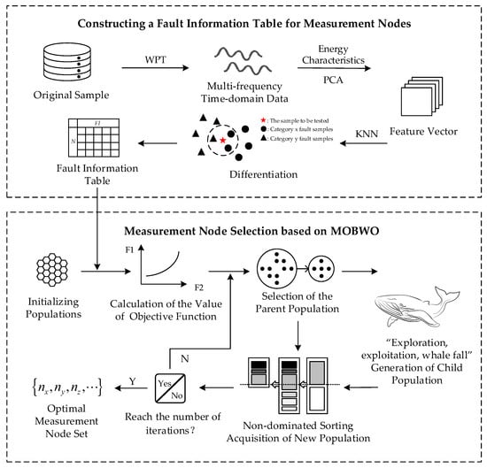
Figure 1.
Block diagram of the measurement node selection method.
The process of constructing the fault information table is as follows. Firstly, a three-layer wavelet packet transform (WPT) is carried out on the original signal, and the energy of the third-layer wavelet packet is calculated as the sample features. Secondly, linear dimensionality reduction is carried out on the energy feature data by principal component analysis (PCA) to obtain the feature vector that contains most of the effective information. Again, the K-nearest neighbors (KNN) algorithm is utilized to classify and predict any two types of faults under each measurement node to obtain the differentiation between faults. Then, the differentiation degree of each measurement node for each type of fault category information is calculated by combining formulae, and the measurement point fault information table is constructed. Finally, the differentiation degree of each measurement node for each type of fault is calculated by combining the formula, and the measurement node fault information table is constructed. Based on the measurement node fault information table, the MOBWO algorithm is utilized for the selection of measurement nodes under multi-objective scenarios, and the trade-off between the number of measurement nodes and the fault information is realized through the design of individual coding, genetic operator and fitness target, and, finally, the optimal set of measurement points is obtained.
2.2. Constructing a Fault Information Table for Measurement Nodes
As can be seen from Section 2.1, the core of constructing a fault information table for measurement nodes is to compute the differentiation between each of the two types of faults. Compared with the integer coding table, the fault differentiation can more accurately reflect the isolation relationship between different faults under the same measurement node, as well as the amount of various types of fault information contained in each measurement node. Therefore, in this paper, the KNN algorithm is used to calculate the differentiation between any two types of faults under each measurement node.
KNN is a supervised learning method based on distance metrics and majority decision making, which requires labeled samples as training data. KNN takes all the samples of known categories as a reference, calculates the distance between the sample to be categorized and all the known samples, and selects the K-nearest known samples from it. According to the voting law of minority–majority, the one that belongs to the largest proportion of categories among the K-nearest neighbor samples is the category of the sample to be classified. A commonly used distance metric is Euclidean Distance [25], and the Euclidean Distance between point and point in n-dimensional space is shown in Equation (1):
The process of using KNN to find fault differentiation is as follows: calculate the Euclidean Distance between the unknown samples in the test set and all the known samples in the training set by using Equation (1) and discriminate the fault types according to the “nearest neighbor” decision rule of the KNN algorithm, and the ratio of the number of correctly categorized samples in the test set to the total number of samples of the two types of faults is the fault differentiation, as shown in Equation (2), where l and m represent a certain two types of fault types. Let the total number of fault types under a measurement node be M and the number of test samples contained in each fault type be . Then, the fault sample vector for categories l and m is , and the prediction result after classification by the KNN algorithm is . Comparing the prediction result with the actual label of the two types of fault samples, the fault discrimination FD is obtained as follows:
Table 1 shows an example of the differentiation of various types of faults for a certain measurement node. The table is a symmetric matrix, where the rows and columns all represent fault categories, and F0 represents the case when the circuit is in a normal state. The numerical values represent the degree of differentiation between the two fault categories, the larger value means that the two faults are differentiated to a higher degree under the current measurement node, where “1” means that the two faults can be completely isolated, and the rest of the values indicate that there are different degrees of confusion between the two fault characteristics.

Table 1.
An example of fault discrimination table for a certain measurement node.
The table of fault differentiation for a single measurement point can reflect the differentiation between a certain type of fault and all other faults. For example, in Table 1, the differentiation between fault F1 and normal state F0 is 0.500, the differentiation between F1 and F2 is 1.000, and the differentiation between F1 and F4 is 0.925, which indicates that F1 and F2 can be completely isolated, and the differentiation between F1 and F0 and F4 is significantly different, although they cannot be completely isolated. Therefore, it can be found that the fault differentiation table can reflect the differentiation relationship between the faults more finely.
Let denote the value corresponding to the row and column in the fault differentiation table of measurement node n1, i.e., the differentiation between fault and fault . Then, the information of a certain type of fault contained in measurement node n1 can be calculated according to Equation (3):
where is the information of class fault contained in measurement node n1, determined by the differentiation between this fault and normal data, as well as other fault data. Where denotes the differentiation between class faults and normal state F0, denotes the summation of the differentiation between class faults and other classes of faults, and N denotes the total number of fault classes containing F0. The weight coefficients and both take the value 0.5.
From the above, the fault information of each measurement node in the circuit can be obtained by Equation (3); however, for complex circuits, the number of measurement nodes included in the optimal measurement node set may be more than one, so the fault information of the measurement node set consists of the maximum value of the corresponding fault information of all measurement nodes. Let the fault information of measurement nodes n1 and n2 be , , then the fault information of measurement node set {n1, n2} is , as shown in Table 2.
Table 2.
Fault information table for n1, n2 and {n1, n2}.
2.3. Measurement Node Selection Based on MOBWO Algorithm
Multiple objective beluga whale optimization (MOBWO) is a multi-objective optimization algorithm proposed by integrating Non-dominated Sorting Genetic Algorithm-II (NSGA-II) on the basis of beluga whale optimization (BWO) [26,27]. The MOBWO algorithm mainly contains the steps of fast non-dominated sorting, crowding distance calculation, child population generation, parent–child merger, and elite strategy selection. Among them, fast non-dominated sorting and crowding distance calculation are the core mechanisms of NSGA-II, which together ensure that the multi-objective optimization algorithm can effectively find the Pareto optimal solution. And BWO, as a genetic operator in the algorithm, updates the positions of individuals in the preferred parent population through the three phases of exploration, exploitation and whale fall to obtain the offspring population. Where the formula for updating individual positions in the exploration stage is shown in Equation (4), the formula for updating individual positions in the exploitation stage is shown in Equation (5), and the formula for updating individual positions in the whale-fall stage is shown in Equation (6).
In Equation (4), denotes the position of the individual on the dimension at the next iteration; denotes the position of the individual on the random dimension under the current iteration; and denotes the position of the random individual on the random dimension under the current iteration. In Equation (6), is the step size of the whale fall.
In the MOBWO-based measurement node selection method, a population of size N represents N possible combinations of measurement nodes, e.g., the combination of measurement nodes is , where is the total number of measurement points. In the genetic algorithm, the commonly used population initialization method is to randomly generate random numbers between [0, 1]; however, there are only two states of measurement nodes, either selected or unselected, so the individuals are encoded through the dichotomous method in this paper. If in the measurement node combination , then it means that the measurement node is selected, and vice versa is not selected. Also based on the analysis of the analog circuit measurement node selection problem, two optimization objectives of the MOBWO algorithm are designed, which are the number of measurement nodes in the measurement node set and the number of fault types in the fault information, as in Equations (7) and (8).
In Equation (7), denotes the number of measurement nodes in the measurement node combination . In Equation (8), denotes the fault information of the class fault under the measurement node set , and denotes the number of types of fault information contained in , where Q is the basis for the determination of the fault discrimination ability of the measurement node set, which can be adjusted according to the actual situation, and, in this paper, based on the detailed analysis of the fault differentiation in multiple circuits, the value is taken as 0.85.
The flowchart of the measurement node selection method based on the MOBWO algorithm is shown in Figure 2.
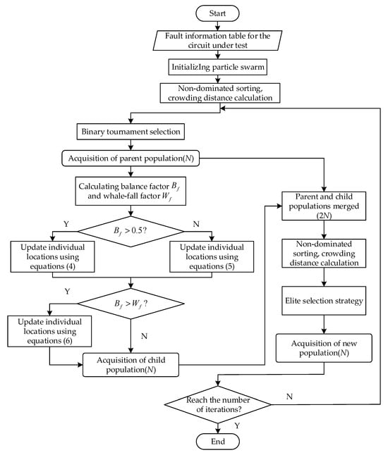
Figure 2.
The flowchart of measurement node selection method.
Firstly, an initial population P0 of size N is randomly generated, and two objective function values are calculated for each individual based on the fault information table of measurement nodes. Secondly, based on these two values, the initial population P0 is subjected to fast non-dominated sorting, crowding distance calculation and ranking, and the individual with the smallest rank or the largest crowding distance when the rank is the same is selected as the parent population by binary tournament selection. Next, the parent population Pt is input into the BWO algorithm, and the child population Qt is generated by the three position update formulas, and then the two populations Pt and Qt are merged to form the population Rt of size 2N. Subsequently, the population Rt is subjected to the fast non-dominated sorting, crowding distance calculation, and ranking, and is retained to generate the next-generation parent by elite selection strategy, and then the process is repeated until the number of iterations reaches a set maximum.
3. Soft-Fault Diagnosis Method
3.1. Fault Diagnosis Model Based on APSO-SDAE
In order to overcome the influence of the weakness of the soft-fault features and realize the accurate identification of components that are in a faulty state in analog circuits, a deep network model that combines APSO and SDAE is proposed in this paper, which includes a total of four modules, including parameter optimization, weight initialization, autoencoder, and classification prediction, and the overall framework of the analog circuit fault diagnosis method based on this model is shown in Figure 3.
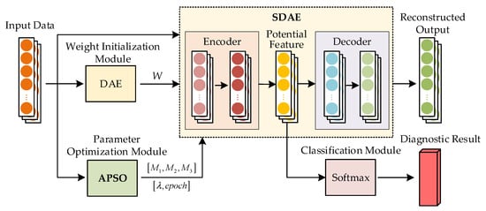
Figure 3.
The overall framework of the analog circuit fault diagnosis method.
As shown in Figure 3, the weight initialization module uses the hierarchical pre-training process of denoising autoencoder (DAE) to obtain the weight W, which is input to the SDAE module as the initial value of the weights between the layers; in the parameter optimization module, an SDAE hyperparameter optimization method based on the APSO algorithm is proposed to obtain the better value of parameter combinations by comparing the failure rate of the classification prediction; finally, a Softmax layer is introduced as a classification module to accomplish the task of fault classification for the raw data of analog circuits.
Stacked noising autoencoder (SDAE) is a deep learning neural network model composed of multiple DAE. Considering that too many implicit layers will have a large impact on the computational rate of the model, the SDAE model containing three implicit layers is used to complete the analog circuit fault diagnosis task. The initial values of the weight parameters in the SDAE model are derived from the DAE hierarchical pre-training process, as shown in Figure 4.
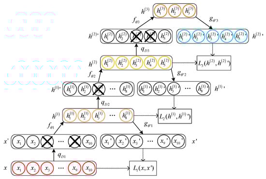
Figure 4.
Schematic diagram of the DAE hierarchical pre-training process.
In Figure 4, x represents the original input data; , , and represent the introduction of noise operations for each DAE layer; , , and represent potential spatial representations; , and represent the reconstructed output data. During the DAE hierarchical pre-training process, each DAE model separately performs an encoding operation and a decoding operation on the broken data after the introduction of noise and updates the weight parameters based on the loss function between the input and the reconstructed output. After the pre-training of all DAEs, the weight matrix of the SDAE model is initialized using the weight parameters in the encoding function and decoding function obtained from the pre-training.
3.2. Optimization of Hyperparameters of SDAE
3.2.1. Core Steps of APSO Algorithm
Particle swarm optimization (PSO) is a global optimization algorithm that simulates the feeding behavior of bird flocks in nature, proposed by Kennedy and Eberhart in 1995. As a group intelligence algorithm, PSO utilizes the sharing of information by individuals in the group to make the movement of the whole group evolve from disorder to order and find the optimal solution to the problem through the joint action of individual experience and group experience. The adaptive particle swarm optimization (APSO) algorithm, as a variant of PSO, consists of two core steps: updating of particle positions and velocities and updating of inertia weights.
- Updating of particle positions and velocities
Like the PSO algorithm, the particles in the APSO algorithm have only two attributes: position and velocity, where the position of each particle represents a solution to be evaluated, and the velocity of the particle determines the direction in which it searches for a new solution and the distance it is about to move. The formulas for updating the velocity and position of the particles in the APSO algorithm are shown in Equation (9):
where is the current iteration number; is the inertia weight; and are the acceleration factors; and are random numbers between [0, 1]; is the individual historical optimal position; and is the global optimal position.
- 2.
- Updating of inertia weights
In the standard PSO algorithm, the inertia weight is an important parameter to control the current speed of the particles, a larger inertia weight can make the particles more inclined to keep the current motion state, which is conducive to improving the global search ability of the algorithm; while a smaller inertia weight can make the particles converge to the individual optimal solution and the global optimal solution more quickly, which is conducive to improving the local improvement ability of the algorithm. Obviously, compared with the fixed value in the standard PSO algorithm, the dynamic in the APSO algorithm can balance the global search and local improvement ability, so that the particle swarm can obtain better optimization results. Therefore, the APSO algorithm in this paper uses the adaptive weighting method to dynamically update so that it can automatically change with the adaptation value of the particle, the specific expression is shown in Equation (10):
where and denote the upper and lower limits of the inertia weights, denotes the current adaptation value of the particle, and and denote the average and minimum of the adaptation values of all particles in the current population.
From Equation (9), for the particle whose current fitness value is better than the average, its updated inertia weight is smaller, thus retaining the particle; while for the particle whose current fitness value is worse than the average, its updated inertia weight is larger, so that the particle can move closer to the better search area.
3.2.2. Optimization Process for SDAE Hyperparameters
The value of hyperparameters in the SDAE model not only affects the model learning ability, but also may cause the model to run for too long. In a single SDAE model, the hyperparameters that affect model performance often require multiple preliminary experiments to determine suitable values. Therefore, the APSO algorithm is used to simultaneously optimize two important hyperparameters of the SDAE model, enabling it to better learn the underlying structure of various fault data in the training set.
Take the number of neurons in the hidden layer, M, the learning rate, , and the number of training rounds, epoch, for example. An increase in M provides more learning capability, but too many neurons may increase the risk of overfitting and the computational cost of the model. The learning rate controls the learning progress of the model, so, if the value of is set too large, the model may ignore the optimal value and fail to converge; similarly, if the value of is set too small, the model will converge too slowly and the computation time will be too long. The number of training rounds is the number of times the entire training data set has been learned, and if the value of epoch is set too large, it may cause the model to overlearn, and vice versa, it may cause the model to fail to adequately learn the data features. Therefore, the selection of appropriate hyperparameters is crucial to achieve the optimal performance of SDAE. In this paper, the APSO algorithm is used to optimize the three hyperparameters, M, , and epoch, in parallel, and the flowchart is shown in Figure 5.
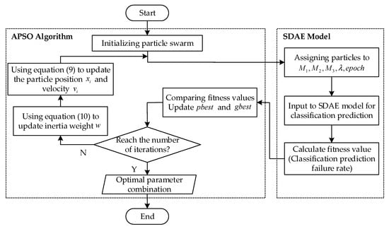
Figure 5.
The hyperparameter optimization process for SDAE model.
Each particle in the APSO algorithm represents a combination of parameters , where M1, M2, and M3 represent the number of neurons in the three hidden layers of the SDAE model, respectively. From Section 3.2.1, the value of the inertia weight w in the APSO algorithm changes with the value of the particle fitness, so before the start of the algorithm iteration, it is necessary to determine a fitness function associated with the optimization objective. In the analog circuit fault diagnosis problem, the ultimate goal of model parameter optimization is to improve the fault diagnosis accuracy; therefore, in this paper, the fitness function is designed as the classification prediction failure rate of the SDAE model under the condition that each particle (parameter combination) is in a different position, and the final optimization goal is the minimum value of the classification prediction failure rate.
3.3. Process of Fault Diagnosis
The process of fault diagnosis for analog circuits based on APSO-SDAE is divided into two phases: offline training and online diagnosis, as shown in Figure 6. In the offline training phase, the APSO algorithm calculates the fitness value of each particle (each parameter combination) based on the training sample data and obtains the optimal parameter combination by taking the minimum of the classification prediction failure rate as the optimization goal, then the SDAE model is initialized based on the four parameters of the weights, the number of neurons in the implicit layer, the learning rate, and the number of training rounds. The weights of the APSO-SDAE model are updated layer by layer according to the classification loss, and, finally, the trained fault diagnosis model is obtained. In the online diagnosis stage, the test sample data are input into the APSO-SDAE fault diagnosis model to obtain the diagnosis results of the soft fault of the circuit under test.
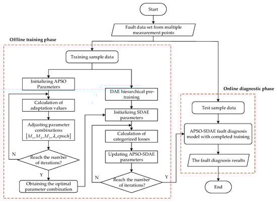
Figure 6.
Fault diagnosis process for analog circuits based on APSO-SDAE.
4. Experimental Verification of Standard Circuits
4.1. Selection and Simulation Settings of Standard Circuits
In order to verify the effectiveness of the method proposed in this paper, two standard circuits commonly used in the field of fault diagnosis are selected as the experimental objects to carry out measurement node selection experiments and fault diagnosis experiments. The schematic diagrams of the four-opamp biquad high-pass (FOBHP) filter circuit and leapfrog filter circuit are shown in Figure 7a,b, and the red numbers represent the measurement nodes of the circuits.
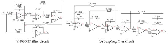
Figure 7.
The schematic diagrams of standard circuits.
In this paper, PSPICE software (OrCAD_Lite_Capture_PSpice 17.2.) is used to simulate the fault types of two standard circuits one by one, in which the excitation signal is selected to be a pulse signal with an amplitude of 5 V, and the pulse signal contains a large number of frequency components, which is conducive to improving the differentiation between different fault types in the circuit. The simulation settings for the measurement node selection experiment and the fault diagnosis experiment are as follows:
- (1)
- In the measurement node selection experiments, the simulation sampling time for each circuit was set to 500 μs and the number of sampling points was 2500. The number of Monte Carlo simulations performed for each fault type is 50, where the tolerance ranges for resistance and capacitance are set to 5% and 10%.
- (2)
- In the fault diagnosis experiments, the simulation sampling time for each circuit was set to 500 μs and the number of sampling points was 1024. The number of Monte Carlo simulations performed for each fault type is 120, where the tolerance ranges for resistance and capacitance are set to 5% and 10%.
4.2. Measurement Node Selection Experiment
4.2.1. Settings of Measurement Node Selection Experiments
Considering that when a hard fault occurs in a component of the circuit, the fault information characteristics from each measurement node are the most obvious, which is conducive to the construction of the measurement node set. Therefore, the single-fault and hard-fault cases of the above two standard circuits are used for the analysis of the optimal set of measurement nodes. The simulation of open-circuit faults is accomplished by component replacement using a resistor with a resistance value of 100G Ω, and, similarly, the simulation of short-circuit faults is accomplished by component replacement using a resistor with a resistance value of 10−6 Ω. The experimental setup for the standard circuits is shown in Table 3.
Table 3.
The experimental setup for the standard circuits.
The fault types for the FOBHP filter circuit are set to non-fault and hard faults of 12 components, and the fault types for the leapfrog filter circuit are set to non-fault and hard faults of 17 components.
4.2.2. Results and Analyses of Measurement Node Selection Experiments
In this section, measurement node selection experiments are performed on two standard circuits to obtain the Pareto front as shown in Figure 8, where F1 and F2 represent two objective function values, which are the number of measurement nodes and the number of fault types contained in the fault information, respectively.
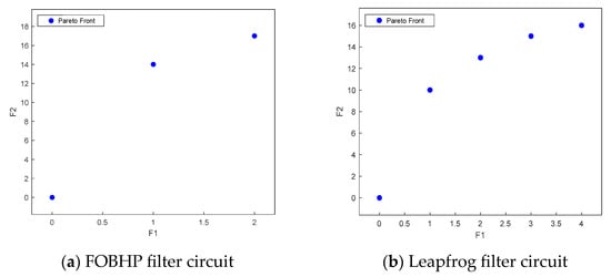
Figure 8.
Pareto front for the MOBWO algorithm.
As can be seen from Figure 8, within a certain limit, the greater the number of measurement nodes, the greater the number of fault types that may be included in the collected data; however, the number of measurement nodes is not the more the better, and, in practical applications, need to be combined with the specific circumstances for the selection of the set of measurement nodes. Take the leapfrog filter circuit as an example, when the number of measurement nodes is 1, the number of faults involved in the sampling data set is 10; when the number of measurement nodes is 4, the number of faults involved in the sampling data set is 16. However, when the number of measurement nodes is increased from 3 to 4, the number of faults only increases by 1. Therefore, the number of measurement nodes needs to be selected reasonably if the test cost of multiple measurement nodes is considered in the actual situation. At the same time, there is no solution in the Pareto front of the leapfrog filter circuit with the number of measurement nodes greater than 4, which indicates that the number of fault types does not increase when the number of measurement nodes continues to increase, which also proves that the measurement node selection method proposed in this paper is able to guarantee the maximum number of fault types when the number of measurement nodes is as small as possible. The optimal set of measurement nodes for the two standard circuits is shown in Table 4.
Table 4.
The optimal set for the measurement node selection method in this paper.
Since the structure of the FOBHP filter circuit is simpler and the number of measurement nodes is less, the information on 17 fault types can be extracted only by the collected data of 2 measurement nodes. On the other hand, the optimal measurement node set of the leapfrog filter circuit has more categories of measurement point combinations, e.g., if the number of measurement nodes is 3, then the optimal set of measurement nodes has three cases, which are {4, 5, 12}, {1, 6, 12}, and {4, 6, 12}, and are arranged according to the crossing distance from top to bottom in Table 4.
In order to verify that the method proposed in this paper can perform the task of multi-objective measurement node selection better, the experimental results of the leapfrog filter circuit are compared with existing methods [19,21], as shown in Table 5.
Table 5.
Comparison of different measurement point selection methods for leapfrog filter circuits.
For this circuit under the same experimental conditions, the number of fault types contained in the fault information of the measurement node set obtained using the method proposed in this paper is better than that of other existing methods, whether in the case of 3 measurement nodes or 4 measurement nodes.
4.3. Fault Diagnosis Experiment
4.3.1. Settings of Fault Diagnosis Experiments
In order to verify the effectiveness of the fault diagnosis method based on APSO-SDAE for the soft-fault diagnosis problem of analog circuits, the 50% parameter shift states of some components in the FOBHP filter circuit and the leapfrog filter circuit are selected as the soft-fault states, and the fault diagnosis experiments and analyses are carried out for two standard circuits. The fault modes of the FOBHP filter circuit are set as non-fault and 16 fault states (C1↓, C2↓, R1↑, R1↓, R2↑, R2↓, R3↓, R4↓, R6↑, R7↑, R7↓, R8↑, R9↑, R9↓, R10↑, R10↓), and the fault modes of the leapfrog filter circuit are set as non-fault and 13 fault states (C1↓, C4↓, R1↑, R1↓, R2↓, R3↑, R4↑, R5↑, R5↓, R7↑, R9↓, R10↓, R11↑). The symbol ↑ indicates that the parameter value of the component is 50% higher than the nominal value, and the symbol ↓ indicates that the parameter value of the component is 50% lower than the nominal value.
From the experimental results of the measurement node selection in Section 4.2.2, it can be seen that the fault data set from multiple measurement nodes will contain more fault information, so for the fault diagnosis experiments of the FOBHP filter circuit and the leapfrog filter circuit, the fault data collection method of multiple measurement nodes is used. Meanwhile, considering that the test cost is higher for the measurement node sets with three or more measurement nodes, and the improvement of the number of types in fault information is less, the case of two measurement nodes for the analog circuits is chosen in this paper. The measurement node set for the FOBHP filter circuit is selected as {4, 8}, and the measurement node set for the leapfrog filter circuit is selected as {6, 12}.
In the parameter optimization module of the fault diagnosis model, the APSO algorithm encodes and iteratively searches for the optimal solution for a set range of parameter combinations in the SDAE model according to the fitness function until it reaches the maximum value of the number of iterations, and the optimal parameter combinations are used for the training process of the SDAE model in the subsequent process. Where the population size of the APSO algorithm is set to 10, the maximum number of iterations is set to 10, the weight range is set to [0.4, 0.9], the fitness function is designed as the failure rate of classification prediction, and the search parameters are set as shown in Table 6.
Table 6.
Search parameter range settings for the APSO algorithm.
After several pre-experiments, other relevant parameters of the fault diagnosis method based on APSO-SDAE are set as follows: the learning rate is set to 0.01, the noise coverage is set to 0.5, and the number of training times is set to 50 during the DAE hierarchical pre-training process.
4.3.2. Results and Analyses of Fault Diagnosis Experiments
In this section, soft-fault diagnosis experiments are conducted on two standard circuits, and the iterative optimization search process of the APSO algorithm in the fault diagnosis model is shown in Figure 9, which shows that the fitness values (classification prediction failure rate) of standard circuits are significantly reduced within the number of iterations, which indicates that the APSO parameter optimization module is able to effectively improve the fault diagnosis capability of the SDAE model.
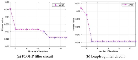
Figure 9.
Iterative optimization process of APSO algorithm.
The optimal parameter combinations of the SDAE model obtained by iterative optimization of the APSO algorithm are shown in Table 7.
Table 7.
Optimal parameter combinations for the SDAE model.
In order to evaluate the diagnostic accuracy of the proposed method, the overall accuracy (OA) of fault diagnosis is used as a performance metric in this section, and the specific formula for OA is as follows:
where TP denotes the number of normal samples judged as normal state, FN denotes the number of normal samples judged as faulty state, FP denotes the number of faulty samples judged as normal state, and TN denotes the number of faulty samples judged as faulty state.
The classification results of the two standard circuits performing the soft-fault diagnosis task are shown in Figure 10. From the overall analysis, the accuracy rates obtained by the APSO-SDAE model on the FOBHP filter circuit and the leapfrog filter circuit reach 97.88% and 98.41%, respectively, indicating that the APSO-SDAE model is able to accurately identify most of the soft-fault types of the FOBHP filter circuit and the leapfrog filter circuit, which exhibits a relatively excellent fault diagnosis performance.
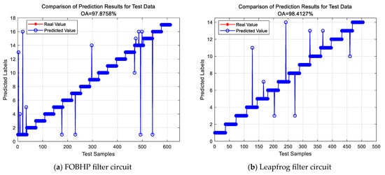
Figure 10.
Fault diagnosis results for standard circuits.
Figure 11 illustrates the confusion matrix for fault diagnosis tasks of two standard circuits, where the blue areas are the correctly classified fault types, while the confusion matrix provides shades of color to represent the percentage of incorrectly classified fault types. In the fault diagnosis experiments, the ratio between the number of samples in the training set and the test set is 7:3, so the number of samples for each type of fault state in the test set is 36. From the confusion matrix, it can be seen that the APSO-SDAE model obtains more accurate diagnostic results for the diagnostic tasks of other fault categories, except for the slightly inferior classification correctness of category 14 (R9↑) and category 1 (NF) in the fault diagnostic task of the FOBHP filter circuit.
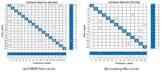
Figure 11.
Confusion matrix for soft-fault diagnosis tasks.
In order to further verify the effectiveness and superiority of the fault diagnosis method proposed in this paper, it is compared with the classification algorithms in the existing methods [1,4,8,16,18], and the results under the same experimental conditions are shown in Table 8. After comparison, it can be concluded that the diagnostic accuracy of the method proposed in this paper is superior to other comparative methods.
Table 8.
Comparison of fault diagnosis results for standard circuits.
In order to reduce the influence of chance factors, 5-fold cross-validation experiments are conducted on the APSO-SDAE fault diagnostic model to evaluate the performance and generalization ability of the model. The results of the 5-fold cross-validation for the FOBHP filter circuit and leapfrog filter circuit are shown in Figure 12. It can be seen that the generalization ability of the APSO-SDAE fault diagnosis model is strong, and the model has a stable effect on the diagnosis of soft faults in analog circuits.
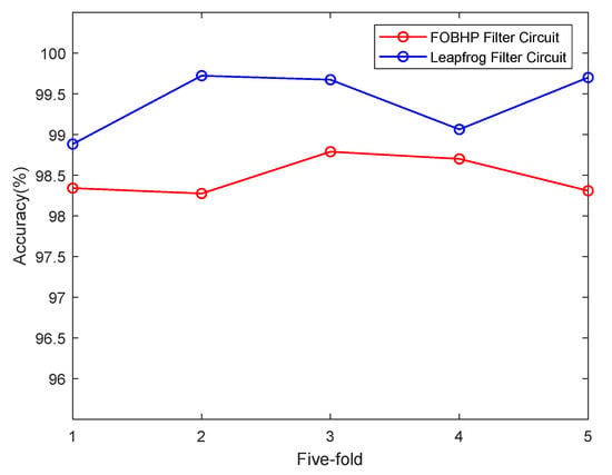
Figure 12.
The 5-fold cross-validation results for APSO-SDAE model.
In order to further verify the innovativeness of the fault diagnosis method proposed in this paper, ablation experiments were conducted for the soft-fault diagnosis task of the FOBHP filter circuit and the leapfrog filter circuit, and the overall fault diagnosis accuracy was adopted as the performance evaluation index. The results of the ablation experiments for the two standard circuits under different measurement node conditions are shown in Table 9.
Table 9.
Results of ablation experiments.
By comparing the fault diagnosis results of the ablation case with those of the complete method, it can be seen that the soft-fault diagnosis accuracy of the FOBHP filter circuit and the leapfrog filter circuit decreases significantly if the APSO parameter optimization module is excluded. By comparing the fault diagnosis accuracy for the single and multiple measurement node cases, it can be concluded that the fault diagnosis results are better under the multiple measurement node conditions.
5. Conclusions
Analog circuits, as an important part of electronic equipment, are widely used in electric power, industry, transportation, medical, aerospace and many other fields, and their reliability directly affects the safe and stable operation of electronic equipment and even the whole system. Therefore, it is of great significance to improve the fault diagnosis level of analog circuits to reduce the maintenance cost of electronic equipment and to reduce the potential hazards brought by soft faults in circuits. In this paper, the optimal measurement node set selection and intelligent fault diagnosis are combined, and on the basis of constructing a fault data set from multiple measurement nodes, combined with a deep learning framework, the research on the analog circuit fault diagnosis method based on the APSO-SDAE is carried out.
- (1)
- Aiming at the status quo that some fault information in analog circuits cannot be extracted from the sampled data of output ports, a test point selection method based on a multi-objective optimization algorithm is proposed. Calculating the fault differentiation to construct the fault information table of measurement nodes, and designing the number of measurement nodes and the number of fault information types as the two objective functions of the multiple objective beluga whale optimization (MOBWO) algorithm in order to achieve the optimal measurement node set selection. In the measurement node selection experiments of two standard circuits, the measurement node set obtained by this method is superior to the comparison methods.
- (2)
- Aiming at the weakness of soft-fault features for analog circuits, a fault diagnosis method based on adaptive particle swarm optimization and stacked denoising autoencoder (APSO-SDAE) is proposed. The APSO parameter optimization module is designed to optimize the SDAE model hyperparameter combinations based on fitness values to improve the fault classification capability. In the soft-fault diagnosis experiments of two standard circuits, the method achieves diagnostic accuracies of 97.87% and 98.41%, respectively, which is about 4% higher than that of the traditional DAE model in dealing with the same fault diagnosis problem, which fully demonstrates that the proposed method is able to identify the soft-fault states of analog circuits effectively.
Author Contributions
Conceptualization, Y.C.; data curation, K.D.; software, Y.X.; validation, B.T. and X.G.; formal analysis, X.X.; investigation, B.T. and Q.W.; writing—original draft preparation, Y.C.; writing—review and editing, X.X. and X.G.; supervision, Q.W.; project administration, Y.C. and K.D. All authors have read and agreed to the published version of the manuscript.
Funding
This research received no external funding.
Data Availability Statement
The authors confirm that the data supporting the findings of this study are available within the article. The experimental object of this study is two standard circuits, the experimental environment is OrCAD_Lite_Capture_PSpice 17.2, and the simulation settings such as excitation signal, sampling time, etc., can be found in Section 4.
Conflicts of Interest
The authors declare no conflicts of interest.
References
- Zhang, C.; Zha, D.; Wang, L.; Mu, N. A Novel Analog Circuit Soft Fault Diagnosis Method Based on Convolutional Neural Network and Backward Difference. Symmetry 2021, 13, 1096. [Google Scholar] [CrossRef]
- Zhang, C.; He, Y.; Yuan, L.; Xiang, S. Analog Circuit Incipient Fault Diagnosis Method Using DBN Based Features Extraction. IEEE Access 2018, 6, 23053–23064. [Google Scholar] [CrossRef]
- Binu, D.; Kariyappa, B.S. RideNN: A New Rider Optimization Algorithm-Based Neural Network for Fault Diagnosis in Analog Circuits. IEEE Trans. Instrum. Meas. 2019, 68, 2–26. [Google Scholar] [CrossRef]
- Yang, H.; Meng, C.; Wang, C. Data-Driven Feature Extraction for Analog Circuit Fault Diagnosis Using 1-D Convolutional Neural Network. IEEE Access 2020, 8, 18305–18315. [Google Scholar] [CrossRef]
- Wang, G.; Tu, Y.; Nie, J. An analog circuit fault diagnosis method using improved sparrow search algorithm and support vector machine. Rev. Sci. Instrum. 2024, 95, 055110. [Google Scholar] [CrossRef]
- Tang, X.; Zhou, X.; Liang, W. Soft Fault Diagnosis of Analog Circuits Based on Classification of GAF_RP Images with ResNet. Circuits Syst. Signal Process 2023, 42, 5761–5782. [Google Scholar] [CrossRef]
- Ding, M.; Ma, R. Fault Diagnosis of Analog Circuits Based on The Sailfish Algorithm Optimized SKELM. J. Phys. Conf. Ser. 2023, 2632, 012014. [Google Scholar] [CrossRef]
- Ji, L.; Fu, C.; Sun, W. Soft Fault Diagnosis of Analog Circuits Based on a ResNet with Circuit Spectrum Map. IEEE Trans. Circuits Syst. I Regul. Pap. 2021, 68, 2841–2849. [Google Scholar] [CrossRef]
- Zhong, K.; Han, M.; Han, B. Data-driven based fault prognosis for industrial systems: A concise overview. IEEE/CAA J. Autom. Sin. 2020, 7, 330–345. [Google Scholar] [CrossRef]
- Wang, H.; Peng, M.; Yu, Y.; Saeed, H.; Hao, C.; Liu, Y. Fault identification and diagnosis based on KPCA and similarity clustering for nuclear power plants. Ann. Nucl. Energy 2021, 150, 107786. [Google Scholar] [CrossRef]
- Yuan, X.; Miao, Z.; Liu, Z.; Yan, Z.; Zhou, F. Multi-Strategy Ensemble Whale Optimization Algorithm and Its Application to Analog Circuits Intelligent Fault Diagnosis. Appl. Sci. 2020, 10, 3667. [Google Scholar] [CrossRef]
- Zhao, S.; Liang, X.; Wang, L.; Zhang, H.; Li, G.; Chen, J. A fault diagnosis method for analog circuits based on EEMD-PSO-SVM. Heliyon 2024, 10, 38064. [Google Scholar] [CrossRef] [PubMed]
- Han, L.; Liu, F.; Chen, K. Analog Circuit Fault Diagnosis Using a Novel Variant of a Convolutional Neural Network. Algorithms 2022, 15, 17. [Google Scholar] [CrossRef]
- Yang, J.; Gao, T.; Jiang, S. A Dual-input Fault Diagnosis Model Based on SE-MSCNN for Analog Circuits. Appl. Intell. 2023, 53, 7154–7168. [Google Scholar] [CrossRef]
- Chen, L.; Khan, U.; Khattak, M.; Wen, S.; Wang, H.; Hu, H. An effective approach based on nonlinear spectrum and improved convolution neural network for analog circuit fault diagnosis. Rev. Sci. Instrum. 2023, 94, 054709. [Google Scholar] [CrossRef]
- Zhong, T.; Qu, J.; Fang, X.; Li, H.; Wang, Z. The intermittent fault diagnosis of analog circuits based on EEMD-DBN. Neurocomputing 2021, 436, 74–91. [Google Scholar] [CrossRef]
- Yang, Q.; Hao, F. Deep auto-encoder network for mechanical fault diagnosis of high-voltage circuit breaker operating mechanism. Paladyn J. Behav. Robot. 2022, 14, 0096. [Google Scholar] [CrossRef]
- Yang, Y.; Wang, L.; Chen, H.; Wang, C. An end-to-end denoising autoencoder-based deep neural network approach for fault diagnosis of analog circuit. Analog. Integr. Circ. Signal Process 2021, 107, 605–616. [Google Scholar] [CrossRef]
- Ma, Q.; He, Y.; Zhou, F.; Song, P. Test Point Selection Method for Analog Circuit Fault Diagnosis Based on Similarity Coefficient. Math. Probl. Eng. 2018, 2018, 9714206. [Google Scholar] [CrossRef]
- Khanlari, M.; Ehsanian, M. A test point selection approach for DC analog circuits with large number of predefined faults. Analog. Integr. Circ. Signal Process 2020, 102, 225–235. [Google Scholar] [CrossRef]
- Zhao, D.; He, Y. A New Test Point Selection Method for Analog Circuit. J. Electron. Test. 2015, 31, 53–66. [Google Scholar] [CrossRef]
- Cui, Y.; Shi, J.; Wang, Z. Analog Circuit Test Point Selection Incorporating Discretization-Based Fuzzification and Extended Fault Dictionary to Handle Component Tolerances. J. Electron. Test. 2016, 32, 661–679. [Google Scholar] [CrossRef]
- Lei, H.; Qin, K. Greedy randomized adaptive search procedure for analog test point selection. Analog. Integr. Circ. Signal Process 2014, 79, 371–383. [Google Scholar] [CrossRef]
- Luo, H.; Lu, W.; Wang, Y.; Wang, L. A New Test Point Selection Method for Analog Continuous Parameter Fault. J. Electron. Test. 2017, 33, 339–352. [Google Scholar] [CrossRef]
- Chen, Q.; Xu, Y. A novel anomaly detection method based on Euclidean distance and deep learning. Neurocomputing 2022, 465, 300–309. [Google Scholar] [CrossRef]
- Deb, K.; Pratap, A.; Agarwal, S.; Meyarivan, T. A fast and elitist multiobjective genetic algorithm: NSGA-II. IEEE Trans. Evol. Comput. 2002, 6, 182–197. [Google Scholar] [CrossRef]
- Zhong, C.; Li, G.; Meng, Z. Beluga whale optimization: A novel nature-inspired metaheuristic algorithm. Knowl.-Based Syst. 2022, 251, 109215. [Google Scholar] [CrossRef]
Disclaimer/Publisher’s Note: The statements, opinions and data contained in all publications are solely those of the individual author(s) and contributor(s) and not of MDPI and/or the editor(s). MDPI and/or the editor(s) disclaim responsibility for any injury to people or property resulting from any ideas, methods, instructions or products referred to in the content. |
© 2025 by the authors. Licensee MDPI, Basel, Switzerland. This article is an open access article distributed under the terms and conditions of the Creative Commons Attribution (CC BY) license (https://creativecommons.org/licenses/by/4.0/).