A Comprehensive Robustness Analysis of Grid-Forming Virtual Synchronous Machine Systems for the Evaluation of Frequency Performance

Abstract

This research proposes a robustness analysis model for the frequency performance of grid-forming converter systems (GFMCS). Based on the derived sensitivity and complementary sensitivity functions, a system robustness identification framework is established. This framework includes two key frequency performance indices: sensitivity and robust stability. Sensitivity analysis is used to describe the system’s sensitivity to external disturbances. In addition, the judgment criterion is proposed to quantitatively and intuitively identify the robustness of the GFMCS. Furthermore, the influence mechanisms of the damping and inertia coefficients on robustness are examined comprehensively. This study finds that when the damping coefficient is small, and the inertia coefficient is large, the system is more prone to oscillatory instability, resulting in longer stability time as well as poorer robustness. Finally, the theoretical analysis is validated experimentally.

1. Introduction

With the increasing severity of environmental pollution and the global energy crisis, renewable energy sources are being widely integrated into modern power systems. This integration is primarily facilitated through power electronics interfaces, leading to significant transformations in the dynamics and stability of power grids [1]. However, unlike traditional power systems dominated by synchronous generators (SG), power–electronics-based renewable energy sources inherently lack inertia, posing challenges to grid stability.

To address these challenges, the concept of the Virtual synchronous generator (VSG) has been introduced. VSG control, also known as virtual inertia control, emulates the dynamic behavior of synchronous generators, thereby enhancing the system’s inertia and damping characteristics. As a result, the stability of grid-forming VSGs has become a crucial research topic, with numerous studies focusing on various aspects of VSG stability, including sensitivity [2,3,4,5,6], robustness [7,8,9,10], and stability analyses [11,12,13,14,15,16,17], categorized by stability analysis type, as shown in Table 1.

Among these topics, sensitivity analysis plays a vital role in evaluating the robustness of GFM-VSG systems. Several studies have investigated the sensitivity of VSG-based grid-forming inverters under varying system conditions [3]. For instance, research has explored the quantitative relationship between model accuracy and input variations, identifying the sensitivity of key control parameters and their impact on system stability [5]. However, existing studies have not fully elucidated the sensitivity of the system’s output response. Additionally, in the context of disturbance sensitivity analysis, a cascaded VSG-based control framework has been proposed, evaluating the sensitivity of VSG converters under varying load conditions and network impedances [2].

Despite these efforts, a standardized criterion for output response sensitivity has not yet been established. While the trajectory sensitivity method has been used to optimize key parameters for adaptive AVSGs (Adaptive virtual synchronous generators) to improve system damping [4], a quantitative evaluation of overall system sensitivity remains absent.

In parallel, studies on robustness analysis have sought to improve VSG system stability. The stability regions of control parameters were investigated in [7], and a novel methodology was developed for designing robust controllers in multivariable systems [8]. Additionally, robust virtual inductor-based power decoupling strategies were explored [9], while a tailored, robust stability analysis method for simplified virtual synchronous compensators was introduced in [10]. However, these studies did not provide a quantitative assessment of system sensitivity and robustness, nor did they comprehensively examine the impact of damping and inertia coefficients on system robustness and dynamic stability.

Another critical challenge in VSG-based systems is low-frequency oscillations, which have been widely studied [18,19,20,21]. Reference [18] investigated the effects of reactive power control and d-q axis voltage control on the oscillatory behavior of VSGs. An adaptive inertia suppression strategy that does not rely on angular velocity derivatives was proposed in [19]. Furthermore, the comparative analysis in [21] highlighted the differences between VSGs and SGs regarding low-frequency oscillation characteristics and damping mechanisms.

In addition, the power coupling effects in VSG-based systems have been the subject of recent studies [22,23,24]. The influence of key control parameters in droop and VSG controllers on power coupling characteristics was explored in [22]. It was also revealed that the coupling between active and reactive power control significantly alters the synchronization stability of VSGs [23]. Moreover, [24] examined the interaction between active and reactive power flows in distributed power systems and its impact on the dynamic behavior of the VSG controller. However, these studies primarily focused on power coupling mechanisms and did not consider the sensitivity of the VSG output response, leaving a crucial gap in the research.

Given these challenges, this study aims to comprehensively analyze the sensitivity of VSG-based grid-forming inverters, providing a quantitative evaluation of output response sensitivity and its implications for system stability. By bridging the gaps in previous research, this work seeks to enhance the robustness and dynamic performance of VSG-controlled power systems.

Table 1. Stability forms.

References	Stability Forms
[3,5,6,22] and this paper	Small Signal Stability
[7,8,23] and this paper	Robust Stability
[9,11,12]	Transient Stability
[13,15,21]	Frequency and Voltage Stability
[10,14]	Fault Ride-Through and System Stability
[18,19,20]	Low-Frequency Oscillation Stability

Table 1. Stability forms.

References	Stability Forms
[3,5,6,22] and this paper	Small Signal Stability
[7,8,23] and this paper	Robust Stability
[9,11,12]	Transient Stability
[13,15,21]	Frequency and Voltage Stability
[10,14]	Fault Ride-Through and System Stability
[18,19,20]	Low-Frequency Oscillation Stability

Based on this background, this study proposes a method for quantitatively analyzing the sensitivity of the output response of the VSG system. The major contributions are organized as follows:

• The sensitivity and robustness impacts of the system can be quantitatively identified through the proposed robustness model, which provides guidance and direction for controller design to mitigate the effects of disturbances on the controller;
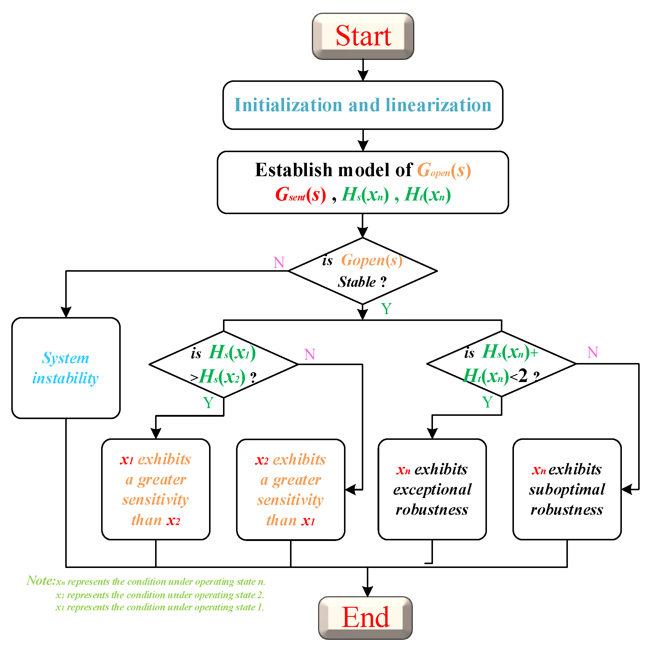
• A judgment criterion for robustness identification is proposed, which can give physical insights into the frequency property of GFMCS subjected to disturbances;
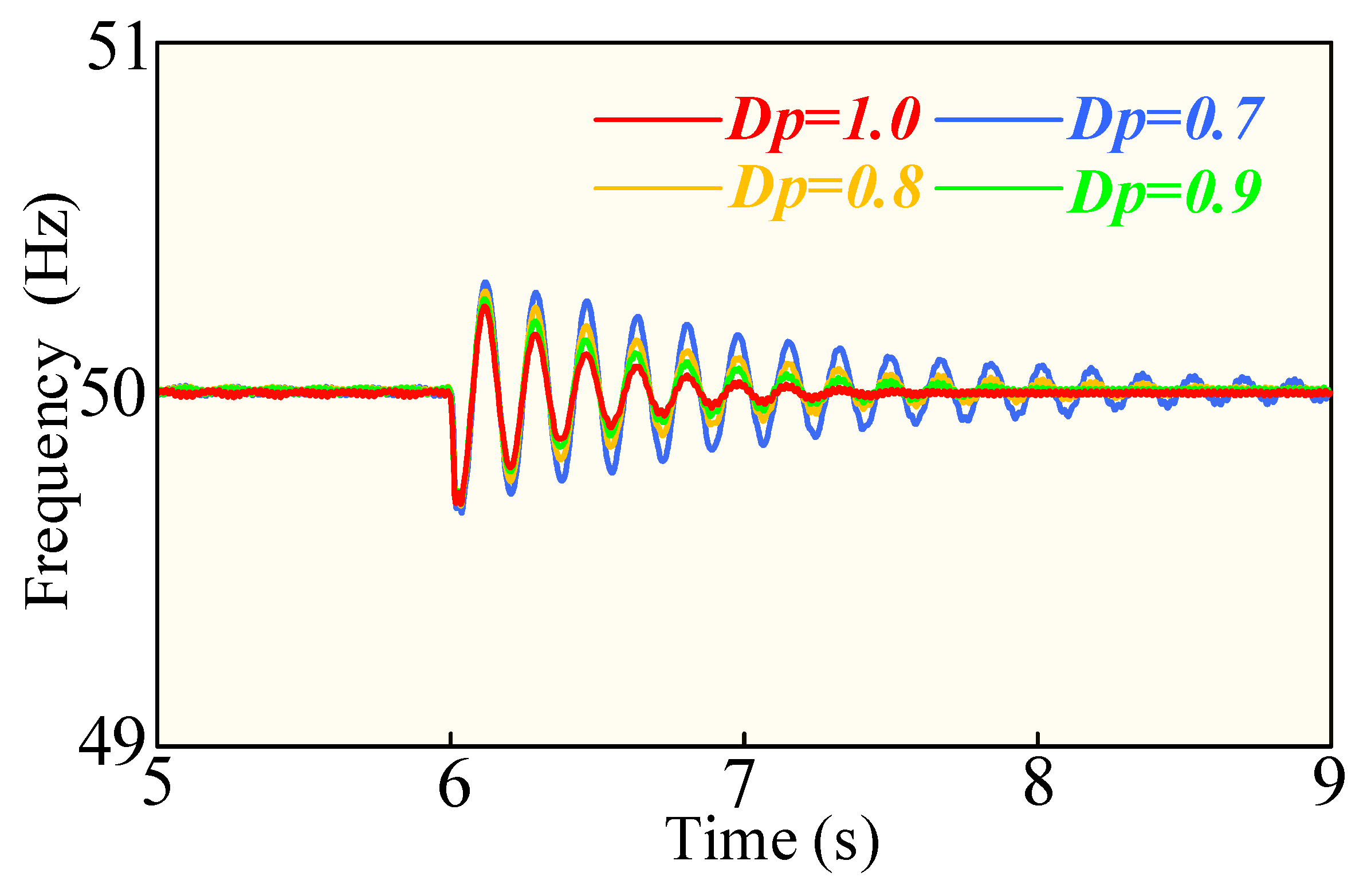
• This study investigates the influence mechanism of damping and inertia coefficients on the robustness of grid-forming converter systems (GFMCS). Optimizing the controller parameters can effectively enhance the dynamic stability and robustness of the system. These contributions provide a theoretical basis and practical guidance for the optimized design of VSG control systems.

The remainder of this study is organized as follows: Section II briefly discusses the basic principles of the grid-forming VSG system. Section III introduces the basic framework of the proposed sensitivity function and comprehensively explains the system sensitivity evaluation mechanism. Section IV presents the validation and analysis of the sensitivity function framework on a simulation platform. Section V provides experimental validation results. Finally, Section VI concludes the research.

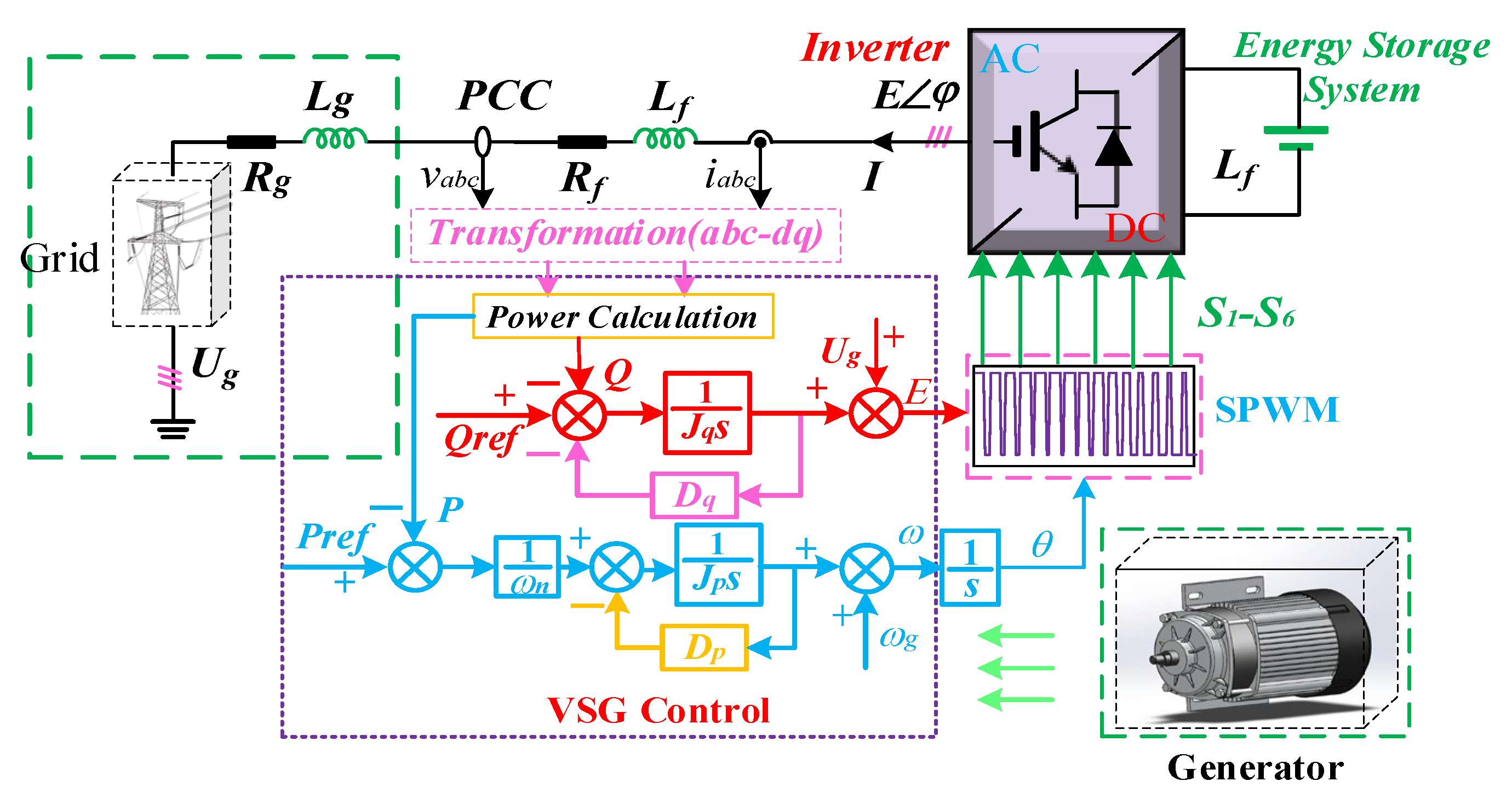
2. Modeling and Sensitivity Analysis of a Grid-Forming VSG System

2.1. A Brief Introduction to VSG

Figure 1 illustrates the topology of a fundamental three-phase grid-connected Virtual synchronous generator (VSG) system. This system emulates the inertia and damping characteristics of a conventional Synchronous generator (SG) and interfaces with the power grid via a three-phase AC inverter. By implementing a dedicated three-phase grid-connected control strategy, the VSG ensures that the grid frequency remains stable at 50 Hz while maintaining a line voltage of 380 V. This contributes to the overall stability and reliable operation of the power grid. Structurally, the VSG topology consisted of two primary components: the circuit and control sections.

The control section was derived from the rotor motion and the voltage amplitude–phase motion equations. The equations are as follows [9]:

$$\left\{\begin{array}{c}{\displaystyle \frac{P_{ref}-P}{{\omega }_n}}=J_p{\displaystyle \frac{d{\theta }^2}{d{t}^2}}\left(\theta -{\theta }_g\right)+D_p{\displaystyle \frac{d\theta }{dt}}\left(\theta -{\theta }_g\right)\\ Q_{ref}-Q=J_q{\displaystyle \frac{dE}{dt}}\left(E-U_g\right)+D_q\left(E-U_g\right)\end{array}\right.$$

(1)

where P_ref represents the reference value of active power, and Q_ref represents the reference value of reactive power. P and Q represent the active power and reactive power calculated through power calculation, respectively. J_p and J_q are the virtual inertia constants of the active and reactive power loops, respectively. D_p and D_q are the damping constants of the active and reactive power loops, respectively. θ and θ_g represent the angular frequencies of the Virtual synchronous generator (VSG) and the grid, respectively. E and U_g represent the magnitudes of the VSG output and the grid voltages, respectively. In particular, U_g is not the voltage value at the PCC. The output voltage at the PCC is fed into the grid through the grid impedance.

Based on Kirchhoff’s voltage law, the electromagnetic model of the VSG system in the d-q coordinate system can be expressed as [9]:

$$\left[\begin{array}{c}{U}_d\\ U_q\end{array}\right]=-\left(R+sL\right)\left[\begin{array}{c}{i}_d\\ i_q\end{array}\right]+\left[\begin{array}{c}{E}_d\\ E_q\end{array}\right]$$

(2)

$$\left\{\begin{array}{c}{E}_d=Ecos\phi \\ E_q=Esin\phi \end{array}\right.$$

(3)

where U_d and U_q represent the d- and q-axis components of the grid voltage in the d-q coordinate system, respectively. Meanwhile, E_d, E_q, i_d, and i_q represent the d- and q-axis components of the VSG output current and output voltage in the d-q coordinate system, respectively. φ is the phase angle between the VSG output and the grid voltages. s is the Laplace operator.

In particular, L and R refer to the total resistance and inductance of the system, where L = L_f + L_g and R = R_f + R_g, as shown in Figure 1. L_f, L_g, R_f, and R_g are all displayed. The output voltage of the VSG is the voltage output from the inverter, where E ∠ φ in Figure 1 represents the output voltage. It should be noted that in this paper, the grid voltage is used as a reference, allowing the assumption that U_q = 0.

By combining Equations (2) and (3), the components of the inverter-side current in the d- and q-axis are given as follows [11]:

$$\left\{\begin{array}{c}\left[\begin{array}{c}{i}_d\\ i_q\end{array}\right]=\left[\begin{array}{cc}{\displaystyle \frac{R+sL}{\left|Z^2\right|}}& {\displaystyle \frac{{\omega }_{n}L}{\left|Z^2\right|}}\\ {\displaystyle \frac{-{\omega }_{n}L}{\left|Z^2\right|}}& {\displaystyle \frac{R+sL}{\left|Z^2\right|}}\end{array}\right]\left[\begin{array}{c}{E}_d-U_d\\ E_q\end{array}\right]\\ Z=\sqrt{R^2+{\left({\omega }_{n}L\right)}^2}\end{array}\right.$$

(4)

where Z is the total impedance of the VSG system.

Based on the instantaneous power theory, the instantaneous active power and reactive power of the VSG is given by:

$$\left[\begin{array}{c}P\\ Q\end{array}\right]=\left[\begin{array}{cc}{e}_d& e_q\\ e_q& -e_d\end{array}\right]\left[\begin{array}{c}{i}_d\\ i_q\end{array}\right]$$

(5)

By performing small-signal linearization on the active and reactive power output of the VSG, the following results were obtained:

$$\left[\begin{array}{c}\Delta P\\ \Delta Q\end{array}\right]=\left[\begin{array}{cc}{E}_d& E_q\\ E_q& {-E}_d\end{array}\right]\left[\begin{array}{c}\Delta i_d\\ {\Delta i}_q\end{array}\right]+\left[\begin{array}{cc}{i}_d& i_q\\ {-i}_q& i_d\end{array}\right]\left[\begin{array}{c}\Delta E_d\\ {\Delta E}_q\end{array}\right]$$

(6)

Since active and reactive powers are transmitted through the grid’s voltage and frequency, there exists a bidirectional coupling effect between them. This coupling effect can be described as follows [11]:

$$\left[\begin{array}{c}P\\ Q\end{array}\right]=\left[\begin{array}{cc}{H}_{11}& H_{12}\\ H_{21}& H_{22}\end{array}\right]\left[\begin{array}{c}\theta \\ E\end{array}\right]$$

(7)

The specific process of active power and reactive power coupling is as follows:

From Figure 2, G₁(s) and G₂(s) are the transfer functions based on the rotor dynamics equation and amplitude–phase dynamics equation in Equation (1), respectively. H₁₁(s) and H₂₂(s) are the transfer functions from the VSG power angle to active power and from voltage to reactive power, respectively. H₁₂(s) and H₂₁(s) represent the transfer functions from the VSG output voltage to active power and from the VSG power angle to active power, respectively.

The components G₁(s), G₂(s), H₁₁(s), H₂₂(s), as well as the power coupling transfer functions H₁₂(s) and H₂₁(s) in Figure 2, are as follows [13]:

$$\left\{\begin{array}{c}{H}_{11}\left(s\right)={\displaystyle \frac{{3\omega }_n(E{U}_g\mathit{sin}\theta \left(R+sL\right)+E{U}_g\cos \mathit{\theta }\left({\omega }_{n}L\right))}{2G_z\left(s\right)}} \\ H_{12}\left(s\right)={\displaystyle \frac{3{\omega }_n(2E-U_g\mathit{cos}\theta \left(R+sL\right)+U_g\mathit{sin}\theta \left({\omega }_{n}L\right))}{2G_z\left(s\right)}}\\ H_{21}\left(s\right)={\displaystyle \frac{3{\omega }_n(-E{U}_g\mathit{cos}\theta \left(R+sL\right)+E{U}_g\mathit{sin}\theta \left({\omega }_{n}L\right)) }{{2G}_z\left(s\right)}}\\ H_{22}\left(s\right)={\displaystyle \frac{3{\omega }_n(2E-U_g\mathit{cos}\mathit{\theta }\left({\omega }_{n}L\right)-U_g\mathit{sin}\theta \left(R+sL\right))}{ {2G}_z\left(s\right)}}\\ G_z\left(s\right)=(s+{\omega }_n)({R+sL)}^2+{\left(s+{\omega }_n\right)\left({\omega }_{n}L\right)}^2 \end{array}\right.$$

(8)

$$\left\{\begin{array}{c}{G}_1\left(s\right)={\displaystyle \frac{1}{\left(J_{p}s+D_p\right){\omega }_{n}s}}\\ G_2\left(s\right)={\displaystyle \frac{1}{\left(J_{q}s+D_q\right)}}\end{array}\right.$$

(9)

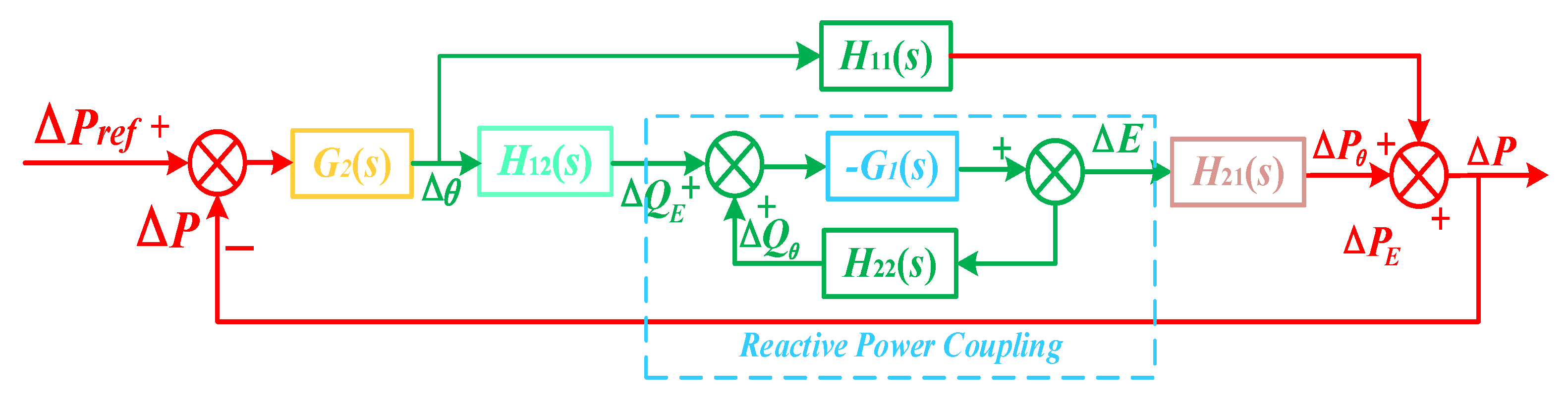
2.2. The Modeling Method for Analysis

Figure 3 presents the control block diagram that accounts for power coupling,G₁(s), G₂(s), H₁₁(s), H₂₂(s), H₁₂(s), and H₂₁(s) can be derived from Equations (8) and (9). G₁(s) is the reactive power coupling part, and G₂(s) is the active power coupling part. The transfer functions H₁₁(s), H₂₂(s), H₁₂(s), and H₂₁(s) correspond to different transmission relationships, where H₁₁(s) represents the transfer from the phase angle to active power, H₂₂(s) describes the transfer from the inverter output voltage to reactive power, H₁₂(s) characterizes the transfer from the phase angle to reactive power, and H₂₁(s) denotes the transfer from the inverter output voltage to active power.

By modifying the control block diagram, the open-loop transfer function can be obtained as follows:

$$G_{open}\left(s\right)={G_2\left(s\right)H}_{11}\left(s\right)-{\displaystyle \frac{G_1\left(s\right){G_2\left(s\right)H}_{12}\left(s\right)H_{21}\left(s\right)}{1+{G_1\left(s\right)H}_{22}\left(s\right)}}$$

(10)

By using the open-loop transfer function, the stability of the VSG system can be directly assessed.

To further analyze the sensitivity of the model, the sensitivity function and complementary sensitivity function are defined as follows:

$$\left\{\begin{array}{c}{G}_{sent}\left(s\right)={\displaystyle \frac{1}{1+G_{open}\left(s\right)}}\\ G_{ten}\left(s\right)={\displaystyle \frac{G_{open}\left(s\right)}{1+G_{open}\left(s\right)}}\end{array}\right.$$

(11)

where $G_{sent}\left(s\right)$ is the sensitivity function, and $G_{ten}\left(s\right)$ is the complementary sensitivity function.

Using Equation (11), we can conduct an in-depth analysis of the sensitivity of the entire Virtual synchronous generator (VSG) system. Sensitivity is an important indicator for measuring the degree to which the system responds to changes, and it provides an intuitive reflection of the VSG system’s damping characteristics under various conditions. Specifically, the magnitude of sensitivity determines the speed at which the system recovers its equilibrium and its stability when facing disturbances or changes. When the sensitivity function has a relatively high value, the VSG system can respond swiftly to external disturbances and restore stability more quickly. Conversely, when the sensitivity function value is low, the system reacts more slowly, which may result in prolonged oscillations or even instability. It is important to highlight that the disturbance discussed in this paper specifically refers to the grid-side inductance disturbance, namely the Lg disturbance.

K_sent(x_n) and K_ten(x_n) define the sensitivity function and complementary sensitivity function as the magnitude of the VSG system’s response under condition x_n. x_n refers to the operating conditions of the system under different parameter conditions. These parameters may include the system’s damping coefficient, inertia coefficient, etc.

$$\left\{\begin{array}{c}{K}_{sent}\left(x_n\right)=20\lg \left|{G_{sent}\left(s\right)|}_{s=j{\omega }_c}\right|\\ K_{ten}\left(x_n\right)=20\lg \left|{G_{ten}\left(s\right)|}_{s=j{\omega }_c}\right|\end{array}\right.$$

(12)

where ω_c is the angular velocity corresponding to the oscillation frequency point of the VSG output variable under condition x_n. $K_{sent}\left(x_n\right)$ and $K_{ten}\left(x_n\right)$ are the magnitudes of the sensitivity function and complementary sensitivity function of the VSG system, respectively.

In robust control, the infinity norms of the sensitivity function and the complementary sensitivity function are often used to evaluate system performance or robustness. A larger infinity norm indicates that the system is more sensitive to disturbances in certain frequency ranges.

In combination with Equation (11), the peak value of the sensitivity function H_s$\left(x_n\right)$ and the peak value of the complementary sensitivity function H_t can be defined as follows:

$$\left\{\begin{array}{c}{H}_s\left(x_n\right)=max\left|G_{sent}\left(j\omega \right)\right|\\ H_t\left(x_n\right)=max\left|G_{ten}\left(j\omega \right)\right|\end{array}\right.$$

(13)

The peak value of the sensitivity function H_s(x_n) is a key indicator for evaluating the robustness of the system, while the peak value of the complementary sensitivity function H_t(x_n) reflects the system’s sensitivity to high-frequency signals. The sum of H_s(x_n) and H_t (x_n) should not be too large, otherwise, both the stability and performance of the system will be compromised, thereby affecting the system’s robustness. The constraint condition is as follows:

$$H_s\left(x_n\right)+H_t\left(x_n\right)<2$$

(14)

Figure 4 presents the flowchart of the judgment process for VSG response sensitivity and robustness, where the sensitivity magnitude of the VSG output response can be quantitatively determined by H_s(x_n). The robustness of the VSG system can be determined by evaluating whether the sum of the magnitude of the sensitivity function and the complementary sensitivity function at the oscillation frequency point is less than 2.

The procedure of judgment and criterion is summarized as follows:

Step 1: Initialization and linearization, and to establish the model of G_open(s), G_sent(s), H_s(x_n), and H_t(x_n).

Step 2: To judge whether G_open(s) is stable or not. If G_open(s) is stable, then jump to Step 3.1. Otherwise, then jump to Step 3.2.

Step 3.1: Further judgment is made to compare which K is larger under condition x₁ and condition x₂. If H_s(x₁) corresponding to condition x₁ is larger, it indicates that under condition x₁, the VSG system’s response speed and sensitivity are faster, the adjustment time is shorter, and the system can reach a stable state more quickly. Similarly, if H_s(x₂) corresponding to condition x₂ is larger, it indicates that under condition x₂, the VSG system’s response speed and sensitivity are faster, the adjustment time is shorter, and the system can reach a stable state more quickly. If the sum of the magnitudes of the sensitivity function and the complementary sensitivity function at the oscillation frequency point is less than 2, the system exhibits strong robustness. Otherwise, the robustness is relatively weak.

Step 3.2: This indicates that the VSG system is in an unstable state, where the output variables may experience synchronous instability or divergent oscillations. In this state, the sensitivity magnitude of the VSG output response is not considered

NOTE: When H_s(x₁) = H_s(x₂), it indicates that the VSG output response sensitivity under conditions x₁ and x₂ is the same. It is important to note that the same sensitivity does not imply that the magnitudes of the output variables are the same. Sensitivity is merely a measure of the speed at which the VSG system’s output converges.

Motivation for the proposed model: Although the open-loop transfer function can analyze the frequency stability margin and dynamic characteristics, it is challenging to evaluate the sensitivity and robustness mechanisms of the output response under different input conditions. Based on this, this paper proposes a model to elucidate the sensitivity and robustness mechanisms of the output response under varying inputs. This method not only considers the system’s steady-state behavior but also emphasizes its dynamic response. It also reveals the system’s ability to recover and its sensitivity. This analytical approach provides clearer guidance for control strategies, especially for enhancing robustness in complex environments.

3. Sensitivity Analysis

To verify the accuracy of the proposed model, the damping coefficient of the active power in the VSG control loop was varied, and the following waveform diagrams were obtained.

Figure 5 shows the waveform of the VSG output frequency under different damping coefficients of the active power loop. It is worth emphasizing that Figure 5 is based on the VSG model shown in Figure 1 and presents the frequency waveform obtained by sampling the output f of the active power control loop, with D_p = 1.0, D_p = 0.9, D_p = 0.8, and D_p = 0.7. It can be seen that as the damping coefficient of the active power loop gradually decreased, the extent of frequency fluctuations also intensified. Since D_p is the feedback-damping loop coefficient and has little impact on the oscillation frequency of the VSG output, the oscillation frequency of the output remained essentially unchanged. This is well verified in Figure 5, where the periods of the output frequency under each D_p value were essentially the same.

The sensitivity function in (12) directly reflects the attenuation rate of the VSG output variable. The larger the value of K_sent(x_n), the slower the attenuation. As shown in Figure 4, with an increase in D_p, the attenuation rate of the VSG output frequency gradually accelerated, and the stability improved. It can be inferred that the value corresponding to the sensitivity function K_sent(x_n) gradually increases.

Figure 6 shows the bode plot of the sensitivity function under different damping coefficients of the active power loop.

From Figure 6, it can be seen that as D_p increased, the bode plot of the sensitivity function showed a gradual decrease in magnitude at the oscillation frequency point. When D_p = 0.7, the magnitude at the corresponding oscillation frequency point was 22.3 dB, and the corresponding K_sent(D_p = 0.7) = 22.3. The maximum sensitivity function indicated slower attenuation, which means the VSG output was more unstable. Figure 4 shows that when D_p = 0.7, the oscillation amplitude was the largest, and the system decayed the slowest, which corresponded to and verified the accuracy of the model. Correspondingly, K_sent(D_p = 0.8) = 19.6, K_sent(D_p = 0.9) = 17.6, and K_sent(D_p = 1.0) = 16.1. The decay rate gradually slowed as K_sent(x_n) increased, which corresponds exactly with Figure 5. Therefore, this verified the correctness of the model.

The trend diagram of the characteristic root changes with varying D_p is shown in Figure 7. According to classical control theory, a characteristic root in the left half-plane indicates that the system is stable, and the closer the dominant pole is to the imaginary axis, the poorer the stability. As shown in Figure 7, as D_p gradually increased, the dominant pole moved further away from the imaginary axis in the left half-plane, indicating that the frequency response of the VSG output became increasingly stable. Another point of verification was that we defined the vertical coordinate of the characteristic root of the dominant pole as the oscillation frequency point of the output response. As shown in Figure 7, as D_p gradually increased from 0.7 to 1.5, the vertical coordinate of its dominant pole remained nearly constant, indicating that the oscillation frequency point of the VSG output response remained unchanged during the variation in D_p. Figure 5 further verifies this point, as the oscillation periods under each set of conditions were essentially consistent. This fully validated the correctness of the sensitivity model.

The dashed lines in Figure 7 represent iso-damping ratio lines, defined as $\mathsf{\zeta }=-{\displaystyle \frac{Re\left(s\right)}{\left|s\right|}}$ When ζ = 0: The system is undamped, with poles located on the pure imaginary axis, resulting in sustained oscillations. 0 < ζ < 1: The system is underdamped, with poles in the left half-plane, leading to damped oscillations. ζ = 1: The system is critically damped, exhibiting no oscillations and fast convergence. ζ > 1: The system is overdamped, with a slower response but no oscillations.

Similarly, the correctness of the model can also be validated by varying the inertia coefficient of the active ring.

Figure 8 presents the frequency simulation waveforms under different inertia coefficients. It can be observed that when J_p = 0.05, the oscillation period of the waveform was the shortest, but the decay rate was the fastest. As J_p increased, the oscillation period gradually lengthened, and the decay rate decreased correspondingly. It can also be inferred that the sensitivity decreases as J_p increases, leading to a weaker stability of the VSG output.

Figure 9 illustrates the bode plot of the sensitivity function of the active power loop under different inertia coefficients. It can be observed that when J_p = 0.15, the sensitivity function reached its maximum value, indicating that the output response had a slower decay rate, a longer settling time, and weaker system stability. As shown in Figure 8, when J_p = 0.15, the decay rate was slower, and the stability was poorer. This observation was consistent with the bode plot and serves to validate the correctness of the model.

However, as J_p gradually decreased from 0.15 to 0.05, the sensitivity function value simultaneously decreased from 21.2 dB to 17.1 dB. This suggests that the decay rate of the VSG output response increased, and the stability improved. The above inference was consistent with the decay rate characteristics observed in the waveform diagram of Figure 8, further validating the correctness of the model.

Figure 10 illustrates the trend of the characteristic roots as J_p increased. As J_p gradually increased from 0.05 to 0.15, the dominant pole moved toward the imaginary axis in the left half-plane, indicating a gradual deterioration in the stability of the output response. This corresponded to the bode plots of the sensitivity function and the frequency response waveforms shown in Figure 8 and Figure 9. Additionally, it is evident that the imaginary part of the characteristic roots decreased with increasing J_p, suggesting a reduction in oscillation frequency and an increase in the oscillation decay period. This was consistent with the observation in Figure 8, where the decay oscillation period increased as J_p increased. The dashed lines in Figure 10 have the same significance as those in Figure 7.

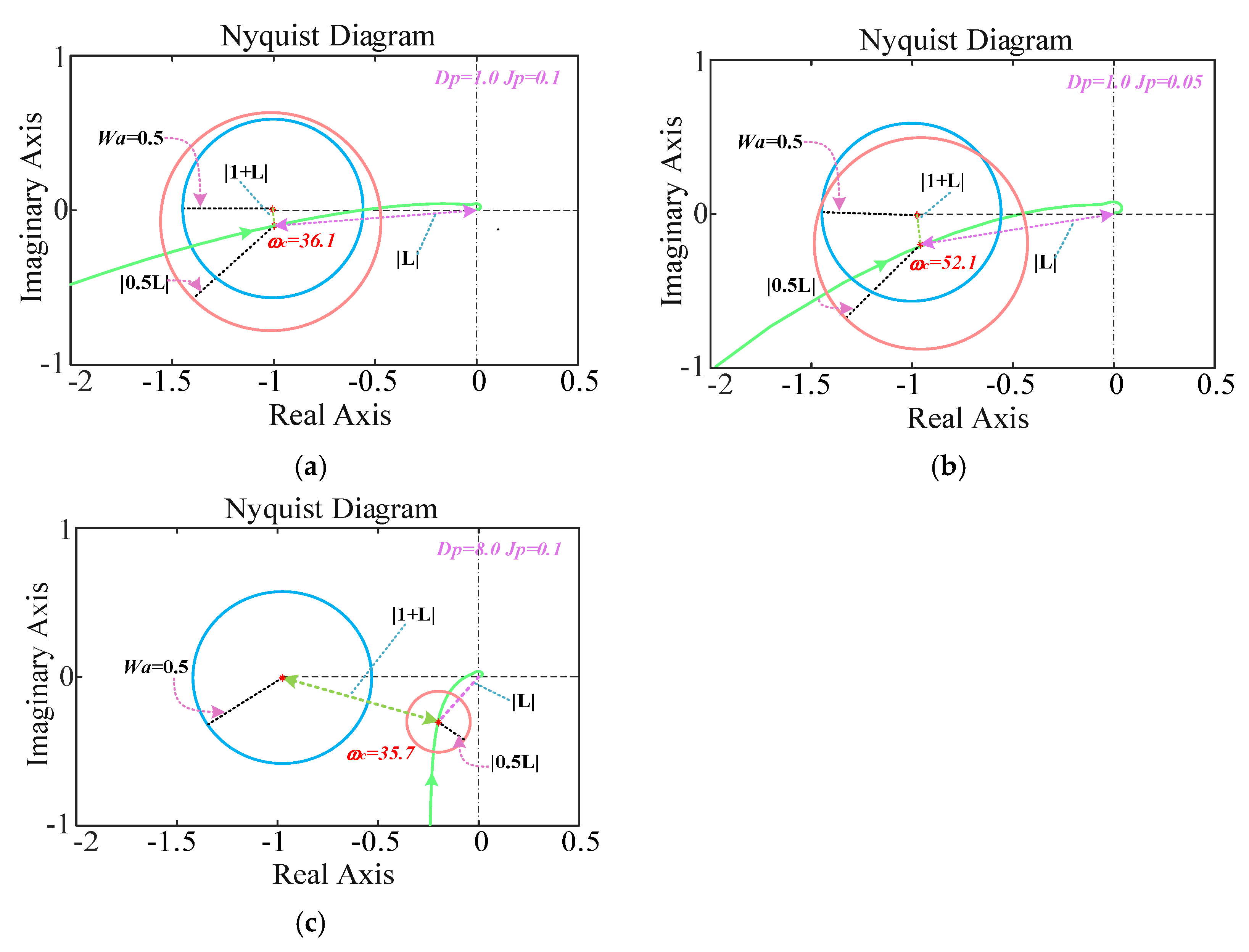
4. Robustness Analysis

Since all the above operating conditions exhibited stable attenuation, the system’s robustness can be analyzed to further enhance its stability.

To ensure system robustness, it was necessary to clearly define and control the possible range of parameter uncertainties. Structured uncertainty modeling and analysis can be considered, which include multiplicative uncertainty and additive uncertainty. Multiplicative uncertainty is more suitable for describing high-frequency model errors or frequency-dependent dynamic uncertainties and can be defined as follows:

$$\left\{\begin{array}{c}{Y}_c=\left|G_0\left(s\right)\left(1+\Delta \left(s\right)\right)\right|\\ \left|\Delta \left(j\omega \right)\right|\le W_m\left(j\omega \right)\end{array}\right.$$

(15)

where G₀(s) is the nominal transfer function, and Δ(s) is the multiplicative uncertainty (typically an unknown but bounded function) that describes the deviation of the actual system from the nominal model.$W_m\left(j\omega \right)$ is the uncertainty weight function.

Based on this, the condition for robust stability is given as follows:

$$\left|G_{ten}{\left(j\omega \right)W}_m\left(j\omega \right)\right|<1 \forall \omega$$

(16)

Then, additive uncertainty in structured uncertainty can be used to analyze the nominal performance of the system. Additive uncertainty is more suitable for describing low-frequency model errors and can be defined as follows:

$$\left\{\begin{array}{c}{Y}_j=\left|G_0\left(s\right)+\Delta \left(s\right)\right|\\ \left|\Delta \left(j\omega \right)\right|\le W_a\left(j\omega \right)\end{array}\right.$$

(17)

where G₀(s), Δ(s) are consistent with the functions in Equation (15), and the $W_a\left(j\omega \right)$ is the uncertainty weight function.

Under the additive uncertainty model, the condition for robust stability of the system is given as follows:

$$\left|G_{sent}{\left(j\omega \right)W}_a\left(j\omega \right)\right|<1 \forall \omega$$

(18)

Based on this, the robustness of the system can be analyzed by plotting the Nyquist curve of the nominal system’s open-loop transfer function, which illustrates the variation in open-loop gain and phase with frequency.

Considering both multiplicative and additive uncertainties, the magnitude of the multiplicative uncertainty weight function $W_m\left(j\omega \right)$ and the additive uncertainty weight function $W_a\left(j\omega \right)$ can be equal to a constant, provided that they satisfy the conditions of Equations (14)–(18). To simplify the model analysis, let $\left|W_a\left(j\omega \right)\right|=\left|W_m\left(j\omega \right)\right|=0.5$.

By combining Equations (16) and (18), the system can maintain stability and performance in the presence of uncertainties, ensuring robust performance, if the following inequalities are satisfied:

$${\left|G_{open}{\left(j\omega \right)W}_m\left(j\omega \right)\right|}_{max}+{\left|G_{open}{\left(j\omega \right)W}_a\left(j\omega \right)\right|}_{max}<1$$

(19)

The robust stability of the system can be determined by examining whether the Nyquist curve enclosed the point (−1, 0). For instance, when the Nyquist curve encloses (−1, 0) on the left half of the complex plane, the system’s robust stability is relatively weak. In contrast, when the Nyquist curve passes through (−1, 0) on the right side without enclosing it, the system’s robust stability is relatively strong.

Figure 11 shows the Nyquist plots under different damping coefficients and inertia coefficients. The blue circles represent additive uncertainty, while the red circles represent multiplicative uncertainty. Therefore, the radius of the blue circle was $\left|W_a\left(j\omega \right)\right|=0.5$, the radius of the corresponding red circle was $\left|G_{open}{\left(j\omega \right)W}_m\left(j\omega \right)\right|=\left|{\displaystyle \frac{G_{open}\left(j\omega \right)}{2}}\right|$. The center of the blue circle was at (−1, 0), while the center of the red circle was the point on the Nyquist curve at the oscillation frequency. According to the physical meaning of Equation (19), when the red circle intersects with the blue circle, it indicates that the system’s robustness is relatively weak. In contrast, when the red circle does not intersect with the blue circle, it indicates that the system’s robustness is relatively strong. It is important to note that when the relationship between the red and blue circles is contained, this indicates that the system’s robustness is weak.

As depicted in Figure 11a, when Dp = 1.0, the Nyquist curve did not encircle the critical point (−1, 0), signifying that the system remained in a stable state and exhibited commendable robust stability. Notably, the red circle was entirely contained within the blue circle, a condition defined as a specific form of intersection. Under these circumstances, the system demonstrated relatively weak robustness. As Dp increased to 8.0, as shown in Figure 11c, the Nyquist curve continued to avoid encircling the critical point (−1, 0), indicating that the system maintained favorable robust stability. Moreover, the blue circle and red circle no longer intersected, further substantiating the enhanced robustness of the system. An additional significant observation is that, with an increase in Dp, the intersection of the open-loop Nyquist curve with the X-axis progressively shifted farther away from (−1, 0), thereby reflecting an improvement in system stability.

As shown in Figure 12a, the peaks of the bode plots of the sensitivity function and complementary sensitivity function were both greater than 1, with values of 16.1 dB and 15.9 dB, respectively. By performing the inverse logarithmic operation, gains of greater than 1 were easily obtained for both. This did not satisfy the robustness stability condition in Equation (14). $H_s\left(x_n\right)+H_t\left(x_n\right)>2$ which resulted in poor robustness of the system. In this case, the robustness was poor. Interestingly, as D_p increased, the system stability gradually improved, and the peaks of the bode plots of the sensitivity function and complementary sensitivity function decreased. As shown in Figure 12c, the peaks of the sensitivity function and complementary sensitivity function were reduced to around 0 dB. By performing the inverse logarithmic operation, gains of less than 2, i.e., $\left(H_s\left(x_n\right)+H_t\left(x_n\right)<2\right),$ were easily deduced, which led to improved robustness of the system. The good robustness in this case was also well validated in the phenomena presented in Figure 11a,c.

It is worth noting that the oscillation angular velocities in Figure 12a–c were 36.1 rad/s, 51.9 rad/s, and 36.7 rad/s, respectively, which corresponded to the oscillation angular velocity points in Figure 11a–c, further verifying the correctness of the model.

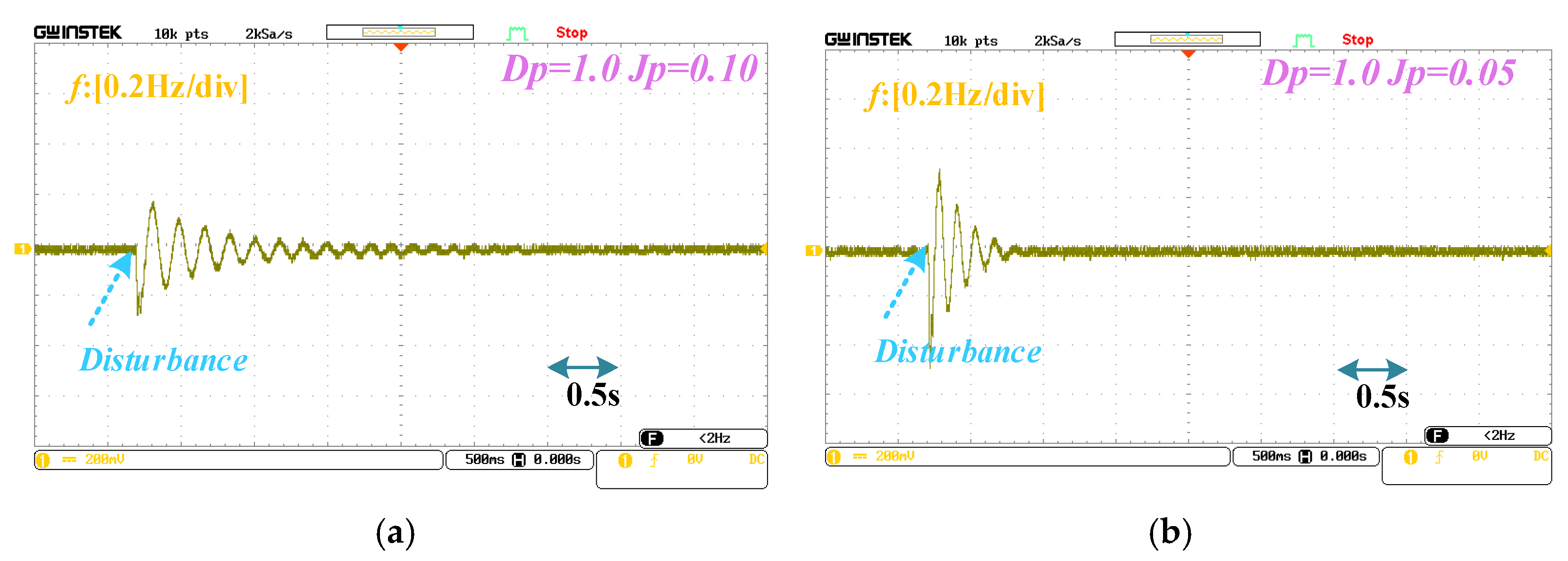
5. Experimental Validation

Figure 13 presents the experimental results, where Cases 1 to 4 corresponded to a gradual decrease in D_p. The experimental setup was based on the topology and control scheme shown in Figure 1. The results indicated that in Cases 1, 2, 3, and 4, the VSG frequency output response exhibited oscillations, with the oscillation amplitude gradually decreasing as D_p increased and the settling time of the damped oscillations increased. These experimental results were consistent with the simulation results, thus validating the correctness of the model.

Similarly, Figure 14 illustrates the experimental results, where Cases 1 to 4 corresponded to a gradual increase in J_p. The experimental setup followed the topology and control scheme presented in Figure 1. The results showed that in Cases 1, 2, 3, and 4, the VSG frequency output response exhibited oscillations, with the settling time of the damped oscillations progressively lengthening as J_p increased. These experimental findings were aligned with the simulation results, thereby confirming the accuracy of the model.

Figure 15 presents the experimental results, where Cases 1 and Cases 2 exhibited oscillations under disturbances, indicating poor system robustness. This was well verified by Figure 12a,b. In contrast, Case 3 showed almost no oscillations under disturbances, suggesting that the system exhibited strong robustness in this scenario. This aligned with the validation provided by Figure 11c and Figure 12c, confirming the correctness of the proposed model.

In summary, the introduction of the sensitivity function and robustness analysis method enabled a qualitative study of the sensitivity and robustness of the VSG output response, allowing for an accurate evaluation of the stability and robustness of the VSG system under different operating conditions. This provided a theoretical foundation for further enhancing the synchronization performance of the VSG with the power grid.

6. Conclusions

This research proposed a new model framework, where a sensitivity function and robustness analysis method were defined to evaluate the sensitivity and robustness of the VSG frequency. Furthermore, an intuitive judgment criterion was proposed to identify the robustness and robust stability of the grid-forming converter systems. The study found that smaller damping coefficients and larger inertia coefficients led to oscillation-related instability. Furthermore, under these conditions, the system’s sensitivity decreased. Additionally, as the damping coefficient increased, the system’s robustness gradually improved.

The research further revealed that an increase in the value of the system’s sensitivity function prolonged the time required to achieve a stable state, thereby deteriorating system stability. Conversely, a decrease in the sensitivity function value shortened the time needed to achieve stability and enhanced system stability. Hence, the sensitivity function serves as a critical metric for evaluating system robustness. When combined with the complementary sensitivity function, it provides a direct approach for robustness analysis, offering a physical insight for optimizing system control parameters, improving system stability, and accelerating response dynamics.

References

1. Blaabjerg, F.; Yang, Y.; Ma, K. Power electronics—Key technology for renewable energy systems—Status and future. In Proceedings of the 2013 3rd International Conference on Electric Power and Energy Conversion Systems, Istanbul, Turkey, 2–4 October 2013; pp. 1–6. [Google Scholar]
2. Liyanage, C.; Nutkani, I.; Meegahapola, L.; Jalili, M. Sensitivity Analysis of the Cascaded Virtual Synchronous Generator based Grid Forming Inverter. In Proceedings of the 2022 IEEE PES 14th Asia-Pacific Power and Energy Engineering Conference (APPEEC), Melbourne, Australia, 20–23 November 2022; pp. 1–6. [Google Scholar] [CrossRef]
3. Tayyab, M.; Awadallah, S.K.E. Investigation of virtual synchronous generator control parameters for small signal stability at different levels of renewable resource penetration. In Proceedings of the 2024 4th International Conference on Smart Grid and Renewable Energy (SGRE), Doha, Qatar, 8–10 January 2024; pp. 1–6. [Google Scholar] [CrossRef]
4. Kuang, Y.; Li, Y.; Wang, W.; Cao, Y. An adaptive virtual synchronous generator control strategy for VSC-MTDC systems and sensitivity analysis of the parameters. In Proceedings of the 2018 13th IEEE Conference on Industrial Electronics and Applications (ICIEA), Wuhan, China, 31 May–2 June 2018; pp. 2631–2635. [Google Scholar] [CrossRef]
5. Zhang, W.; Cui, J.; Zhao, Y.; Yin, H. Parameters Tuning of Flexible Drooped Synchronous Power Controller Based on Small Signal Modeling and Sensitivity Analysis. In Proceedings of the 2023 IEEE 18th Conference on Industrial Electronics and Applications (ICIEA), Ningbo, China, 18–22 August 2023; pp. 886–891. [Google Scholar] [CrossRef]
6. Adu, J.A.; Kyererneh, K.A.; Otchere, I.K. Virtual Synchronous Generator: Parameter Sensitivity Analysis. In Proceedings of the 2021 IEEE 30th International Symposium on Industrial Electronics (ISIE), Kyoto, Japan, 20–23 June 2021; pp. 1–6. [Google Scholar] [CrossRef]
7. Wang, R.; Wang, Y.; Zhang, P.; Sun, Q.; Gui, Y.; Wang, P. System Modeling and Robust Stability Region Analysis for Multi-Inverters Based on VSG. IEEE J. Emerg. Sel. Top. Power Electron. 2024, 12, 6042–6052. [Google Scholar] [CrossRef]
8. Khatibi, M.; Ahmed, S. Robust Controller Design for a Virtual Synchronous Generator (VSG) Using Linear Matrix Inequalities. In Proceedings of the IECON 2020 The 46th Annual Conference of the IEEE Industrial Electronics Society, Singapore, 18–21 October 2020; pp. 3253–3258. [Google Scholar] [CrossRef]
9. Su, H.; Mao, Z.; Li, P. Robust Parameters Based on VSG & Virtual Inductor Design Considering Power Decoupling. In Proceedings of the 2021 IEEE 5th Conference on Energy Internet and Energy System Integration (EI2), Taiyuan, China, 22–24 October 2021; pp. 1185–1190. [Google Scholar] [CrossRef]
10. Mallemaci, V.; Pugliese, S.; Mandrile, F.; Carpaneto, E.; Bojoi, R.; Liserre, M. Robust Stability Analysis of the Simplified Virtual Synchronous Compensator for Grid Services and Grid Support. In Proceedings of the 2023 IEEE Energy Conversion Congress and Exposition (ECCE), Nashville, TN, USA, 29 October–2 November 2023; pp. 1188–1195. [Google Scholar] [CrossRef]
11. Zhu, D.; Ma, Y.; Li, X.; Fan, L.; Tang, B.; Kang, Y. Transient Stability Analysis and Damping Enhanced Control of Grid-Forming Wind Turbines Considering Current Saturation Procedure. IEEE Trans. Energy Convers. 2024. [Google Scholar] [CrossRef]
12. Yang, H.; Chu, Y.; Ma, Y.; Zhang, D. Operation Strategy and Optimization Configuration of Hybrid Energy Storage System for Enhancing Cycle Life. J. Energy Storage 2024, 95, 112560. [Google Scholar]
13. Li, C.; Yang, Y.; Li, Y.; Liu, Y.; Blaabjerg, F. Modeling for Oscillation Propagation with Frequency-Voltage Coupling Effect in Grid-Connected Virtual Synchronous Generator. IEEE Trans. Power Electron. 2025, 40, 82–86. [Google Scholar] [CrossRef]
14. Zhu, D.; Wang, Z.; Hu, J.; Zou, X.; Kang, Y.; Guerrero, J.M. Rethinking Fault Ride-Through Control of DFIG-Based Wind Turbines from New Perspective of Rotor-Port Impedance Characteristics. IEEE Trans. Sustain. Energy 2024, 15, 2050–2062. [Google Scholar]
15. Li, C.; Yang, Y.; Blaabjerg, F. Mechanism Analysis for Oscillation Transferring in Grid-Forming Virtual Synchronous Generator Connected to Power Network. IEEE Trans. Ind. Electron. 2025. [Google Scholar] [CrossRef]
16. Yang, H.; Chen, Q.; Liu, Y.; Ma, Y.; Zhang, D. Demand response strategy of user-side energy storage system and its application to reliability improvement. J. Energy Storage 2024, 92, 112150. [Google Scholar]
17. Li, C.; Yang, Y.; Cao, Y.; Aleshina, A.; Xu, J.; Blaabjerg, F. Grid Inertia and Damping Support Enabled by Proposed Virtual Inductance Control for Grid-Forming Virtual Synchronous Generator. IEEE Trans. Power Electron. 2023, 38, 294–303. [Google Scholar] [CrossRef]
18. Wang, G.; Fu, L.; Hu, Q.; Ma, F.; Liu, C.; Lin, Y. Low Frequency Oscillation Analysis of VSG Grid-Connected System. In Proceedings of the 2021 3rd Asia Energy and Electrical Engineering Symposium (AEEES), Chengdu, China, 26–29 March 2021; pp. 631–637. [Google Scholar] [CrossRef]
19. Zhang, H.; Li, D.; Liu, H.; Sun, D.; Yang, Y.; Shao, Y.; Sun, Y. Comparison of Low Frequency Oscillation Characteristic Differences between VSG and SG. In Proceedings of the 2020 IEEE Sustainable Power and Energy Conference (iSPEC), Chengdu, China, 23–25 November 2020; pp. 668–673. [Google Scholar] [CrossRef]
20. Li, X.; Chen, G. Improved Adaptive Inertia Control of VSG for Low Frequency Oscillation Suppression. In Proceedings of the 2018 IEEE International Power Electronics and Application Conference and Exposition (PEAC), Shenzhen, China, 4–7 November 2018; pp. 1–5. [Google Scholar] [CrossRef]
21. Li, C.; Li, Y.; Du, Y.; Gao, X.; Yang, Y.; Cao, Y.; Blaabjerg, F. Self-Stability and Induced-Stability Analysis for Frequency and Voltage in Grid-Forming VSG System with Generic Magnitude–Phase Model. IEEE Trans. Ind. Inform. 2024, 20, 12328–12338. [Google Scholar] [CrossRef]
22. Li, M.; Wang, Y.; Hu, W.; Shu, S.; Yu, P.; Zhang, Z.; Blaabjerg, F. Unified Modeling and Analysis of Dynamic Power Coupling for Grid-Forming Converters. IEEE Trans. Power Electron. 2022, 37, 2321–2337. [Google Scholar] [CrossRef]
23. Deng, H.; Fang, J.; Tang, Y.; Debusschere, V. Coupling Effect of Active and Reactive Power Controls on Synchronous Stability of VSGs. In Proceedings of the 2019 IEEE 4th International Future Energy Electronics Conference (IFEEC), Singapore, 25–28 November 2019; pp. 1–6. [Google Scholar] [CrossRef]
24. Nascimento, T.F.D.; Salazar, A.O. Power Coupling Influence on Virtual Synchronous Generator Control in Grid-Forming DG Systems. In Proceedings of the 2023 15th Seminar on Power Electronics and Control (SEPOC), Santa Maria, Brazil, 22–25 October 2023; pp. 1–6. [Google Scholar] [CrossRef]
Figure 1. Topological structure and control strategy of the VSG.
Electronics 14 01516 g001
Figure 2. The mutual coupling effect between active and reactive power.
Electronics 14 01516 g002
Figure 3. Active power loop model considering impact of reactive coupling.
Electronics 14 01516 g003
Figure 4. Flowchart of the judgment process for VSG response sensitivity and robustness.
Electronics 14 01516 g004
Figure 5. The simulation waveform of frequency under different damping coefficients.
Electronics 14 01516 g005
Figure 6. The bode plot of the sensitivity function under different damping coefficients of the active power loop.
Electronics 14 01516 g006
Figure 7. The trend diagram of the dominant poles as Dp increases.
Electronics 14 01516 g007
Figure 8. The simulation waveform of frequency under different inertia coefficients.
Electronics 14 01516 g008
Figure 9. The bode plot of the sensitivity function of the active power loop under different inertia coefficients.
Electronics 14 01516 g009
Figure 10. The trend diagram of the dominant poles as Jp increases.
Electronics 14 01516 g010
Figure 11. Schematic representations of system robust stability under different operating conditions. (a) Dp = 1.0, Jp = 0.1, (b) Dp = 1.0, Jp = 0.05, (c) Dp = 8.0, Jp = 0.1.
Electronics 14 01516 g011
Figure 12. Bode diagrams of sensitivity and complementary sensitivity functions under various operating conditions. (a) Dp = 1.0, Jp = 0.1, (b) Dp = 1.0, Jp = 0.05, (c) Dp = 8.0, Jp = 0.1.
Electronics 14 01516 g012
Figure 13. Experiment results: (a) Case 1, (b) Case 2, (c) Case 3, (d) Case 4.
Electronics 14 01516 g013
Figure 14. Experiment results: (a) Case 1, (b) Case 2, (c) Case 3, (d) Case 4.
Electronics 14 01516 g014
Figure 15. Experiment results: (a) Case 1, (b) Case 2, (c) Case 3.
Electronics 14 01516 g015aElectronics 14 01516 g015b
Disclaimer/Publisher’s Note: The statements, opinions and data contained in all publications are solely those of the individual author(s) and contributor(s) and not of MDPI and/or the editor(s). MDPI and/or the editor(s) disclaim responsibility for any injury to people or property resulting from any ideas, methods, instructions or products referred to in the content.