Day-Ahead Optimal Scheduling for a Full-Scale PV–Energy Storage Microgrid: From Simulation to Experimental Validation

Abstract

Microgrids facilitate the complementary and collaborative operation of various distributed energy resources. Implementing effective day-ahead scheduling strategies can significantly enhance the economic efficiency and operational stability of microgrid systems. In this study, the long short-term memory (LSTM) neural network is first employed to forecast photovoltaic (PV) power generation and load demand, using operational data from a full-scale microgrid system. Subsequently, an optimization model for a full-scale PV–energy storage microgrid is developed, integrating a PV power generation system, a battery energy storage system, and a specific industrial load. The model aims to minimize the total daily operating cost of the system while satisfying a set of system operational constraints, with particular emphasis on the safety requirements for grid exchange power. The formulated optimization problem is then transformed into a mixed-integer linear programming (MILP) model, which is solved using a computational solver to derive the day-ahead economic scheduling scheme. Finally, the proposed scheduling scheme is validated through field experiments conducted on the full-scale PV–energy storage microgrid system across various operational scenarios. By comparing the simulation results with the experimental outcomes, the effectiveness and practicality of the proposed day-ahead economic scheduling scheme for the microgrid are demonstrated.

1. Introduction

Since the introduction of the “dual-carbon” goal in China, power generation from renewable energy sources, primarily wind and solar energy, has experienced significant growth [1]. Among these advancements, microgrids have attracted considerable attention and have been actively developed in recent years owing to their capability to efficiently and effectively integrate renewable energy sources at the local level [2]. However, the intermittent and volatile nature of renewable energy generation poses challenges to the operational stability and security of microgrids, particularly when proper scheduling and control mechanisms are not implemented [3]. To address these issues, the integration of energy storage systems into microgrids has proven to be an effective solution. On one hand, the energy storage system can mitigate the uncertainties associated with renewable energy generation, such as that from wind and solar energy sources. On the other hand, the energy storage systems can facilitate complementary and coordinated operation with distributed energy resources, enhancing the stability of microgrid operations and reducing the curtailment of wind and solar energy [4].

The optimal operation and scheduling of microgrids can generally be categorized into two main aspects: the distributed power source side and the load side [5]. On the distributed power source side, the focus lies on achieving complementary and coordinated operation among various generator sets [6]. On the load side, demand response (DR) strategies are primarily considered to optimize energy consumption [7]. For instance, a seasonal optimization framework was proposed for a microgrid incorporating PV power generation and energy storage systems, which investigated the impact of different climatic factors on the optimal configuration of renewable energy [8]. In another study, the slime mold algorithm was employed to achieve the dual optimization of operational costs and carbon emissions through the coordinated operation of battery energy storage systems and distributed generation [9]. Additionally, a DR model based on time-of-use electricity pricing was developed, incorporating factors such as user electricity consumption patterns, consumption elasticity, and peak–valley load behaviors. This model demonstrated that the total cost of the microgrid system could be minimized when 40% of users participated in the DR program [10]. In addition to the economic operation of microgrids, an increasing number of studies have concurrently addressed operational security challenges within microgrids [11,12].

The solution methods for addressing the optimal operation problem of microgrids can be broadly classified into two categories: traditional mathematical programming methods and meta-heuristic algorithms. Traditional mathematical programming methods include techniques such as nonlinear programming [13], the interior point method [14], the alternating direction multiplier method [15], the primal–dual method [16], and dynamic programming [17]. On the other hand, meta-heuristic algorithms include the genetic algorithm [18], particle swarm optimization [19], evolutionary programming [20], the mountain gazelle optimization algorithm [21], and various improved variants of these algorithms. In addition, to address the uncertainties associated with the outputs of distributed energy resources and load demand, common solution approaches include stochastic optimization methods [22] and robust optimization methods [23]. For instance, a multi-stage stochastic programming model was proposed for microgrids integrating multiple types of renewable energy generation, which utilized stochastic dual dynamic programming and Markov chains as a solution [24]. In another study, a two-stage robust day-ahead optimization model for microgrids was developed, employing the column-and-constraint generation algorithm to solve the problem. The validity of the model and algorithm was demonstrated through numerical simulations [25].

Judging from the existing research, most control strategies and day-ahead optimal scheduling schemes for microgrids remain at the simulation verification stage, with limited experimental validation on full-scale microgrids. To address this gap, this study designs an optimal scheduling model for a full-scale microgrid system and conducts field experimental validation. Specifically, an optimization model is developed for a grid-connected photovoltaic–energy storage microgrid, aiming to minimize the daily electricity costs while achieving complementary and coordinated operation among its components. Utilizing historical data from the full-scale microgrid, the PV power and load demand are predicted using the LSTM. The established optimization model is then formulated as a MILP problem and solved using a commercial solver to generate the day-ahead optimal scheduling scheme. Finally, the proposed scheduling scheme is validated through field experiments in the full-scale microgrid. By comparing the actual operation curves with the simulation results, the effectiveness of the proposed day-ahead optimal scheduling scheme is demonstrated.

2. Problem Formulation

As shown in Figure 1, the schematic diagram depicts a full-scale PV–energy storage microgrid within a specific industrial park in Shenzhen, China. The microgrid comprises PV panels, energy storage batteries, and factory machining loads. This microgrid is connected to the main power grid via a transformer, with the entire system managed and controlled by an energy management system (EMS).

The current scheduling and operation mode of the microgrid is described as follows:

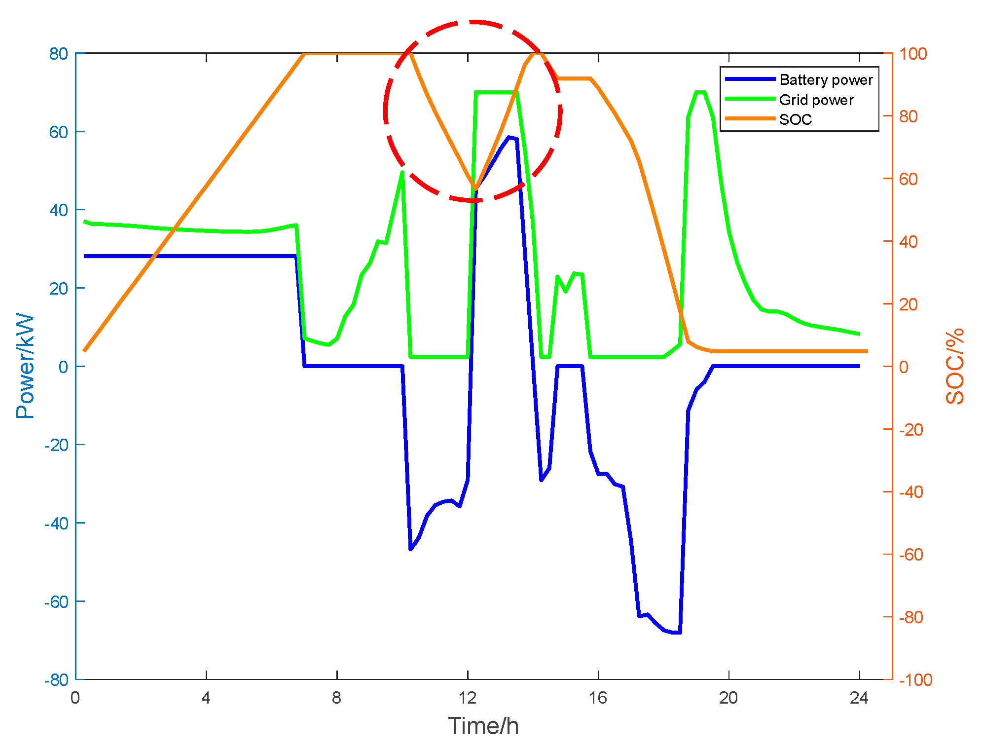
• From 0:00 to 8:00, the energy storage batteries are charged at a constant power rate until they reach their maximum state of charge (SOC).
• From 8:00 to 14:00, the energy storage batteries remain inactive. During this period, the PV power generation and the main power grid jointly supply the load demand, with any surplus PV power being sold back to the main grid.
• From 14:00 to 24:00, the energy storage batteries and the PV power generation work together to supply the load demand until the SOC of the energy storage batteries decreases to its minimum threshold.

Under the current operation mode, the energy storage batteries in the microgrid remain largely inactive between 8:00 and 14:00, both in sunny and cloudy weather conditions. During this period, the load is supplied by PV power generation and the main power grid, with any surplus PV power being sold back to the main grid, as shown in Figure 2a and Figure 2b, respectively.

An analysis reveals that the utilization rate of the energy storage batteries under this operation mode is relatively low. By optimizing the charging and discharging schedules of the energy storage batteries during the morning and noon hours, the daily operating cost of the system can be significantly reduced. To address this, this study proposes a day-ahead optimal scheduling model tailored for this full-scale microgrid.

2.1. Objective Function

The objective function of the proposed optimization model is to minimize the total daily operating cost associated with the full-scale microgrid, as shown below:

$$\min F_c=F_{pen}+{\displaystyle {\sum }_{t=1}^T[C_{buy,t}\cdot P_{n,t}\cdot stat{e}_{n,t}}+C_{sell,t}\cdot P_{n,t}\cdot (1-stat{e}_{n,t})]\cdot \tau$$

(1)

where F_c represents the operating cost of the microgrid for the entire day. T represents the number of time points within a day, and t represents the current time point. P_n,t represents the exchange power between the microgrid and the main grid at the tth time point, where a positive value indicates that the microgrid is absorbing power from the main grid, while a negative value indicates that the microgrid is supplying power to the main grid. The variable state_n,t is a binary variable: a value of 1 indicates that the microgrid is purchasing electricity from the main grid at that moment, while a value of 0 indicates that the microgrid is selling electricity to the main grid. Additionally, C_sell,t and C_buy,t represent the electricity selling price and electricity purchasing price at the tth time point, respectively, and τ represents the time interval. F_pen represents the cost incurred due to changes in the battery state over the course of the day, and its expression is given as follows:

$$F_{pen}={\displaystyle {\sum }_{t=1}^T\left|stat{e}_{b,t}-stat{e}_{b,t-1}\right|}\cdot f_{pen}$$

(2)

where state_b,t is a binary variable: a value of 1 indicates that the battery is currently being charged, while a value of 0 indicates that the battery is being discharged. f_pen represents the cost incurred each time there is a transition between the battery’s charging and discharging states.

2.2. Constraints

The established optimization model, as previously mentioned, must satisfy a set of operational constraints, including system active power balance, limitations on PV power, safety requirements for grid exchange power, and operational constraints for the energy storage battery.

2.2.1. System Active Power Balance Constraints

$$P_{d,t}=P_{s,t}+P_{n,t}-P_{b,t}$$

(3)

Here, P_d,t represents the load demand at the tth time point. P_s,t represents the PV power generation at the tth time point. P_b,t represents the power level of the energy storage battery at the tth time point. A positive battery power value indicates that the battery is in the charging state, while a negative value indicates that it is in the discharging state.

2.2.2. Limitations on PV Power

$$0\le P_{s,t}\le P_{s,\max }$$

(4)

Here, P_s,max represents the maximum PV output of the microgrid system, which is constrained by both the maximum output of the PV panels and the maximum output of the PV inverter.

2.2.3. Safety Requirements for Grid Exchange Power

In the full-scale microgrid, to prevent the battery from feeding power back into the main grid during discharging, the main grid must supply a certain amount of power to the microgrid system. Additionally, to mitigate safety concerns that may arise from the overheating of the grid-connected transformer due to excessive power, and to meet the requirements of the microgrid manager for system security, it is necessary to limit the maximum exchange power between the microgrid and the main power grid, as given below:

$$-P_{n,\max }\cdot stat{e}_{b,t}+P_{n,\lim }\cdot (1-stat{e}_{b,t})\le P_{n,t}\le P_{n,\max }$$

(5)

where P_n,max represents the maximum exchange power between the microgrid system and the main power grid, and P_n,lim represents the grid power necessary to prevent battery backflow.

2.2.4. Operational Constraints for Energy Storage Batteries

$$-P_{b,\max }\le P_{b,t}\le P_{b,\max }$$

(6)

$$SO{C}_t=SO{C}_{t-1}+[(1-{\displaystyle \frac{1}{\eta }})\cdot stat{e}_{b,t}+{\displaystyle \frac{1}{\eta }}]\cdot P_{b,t}\cdot \tau /S_{bat}$$

(7)

$$SO{C}_{\min }\le SO{C}_t\le SO{C}_{\max }$$

(8)

$$SO{C}_{start}=SO{C}_{end}$$

(9)

Here, P_b,max represents the maximum power limit of the battery. η represents the charging and discharging efficiencies of the battery. S_bat represents the capacity of the energy storage battery. SOC_t represents the SOC of the battery at time t. SOC_min and SOC_max represent the minimum and maximum SOC limits of the battery, respectively. SOC_start and SOC_end represent the SOC of the battery at the initial and final moments of a day, respectively.

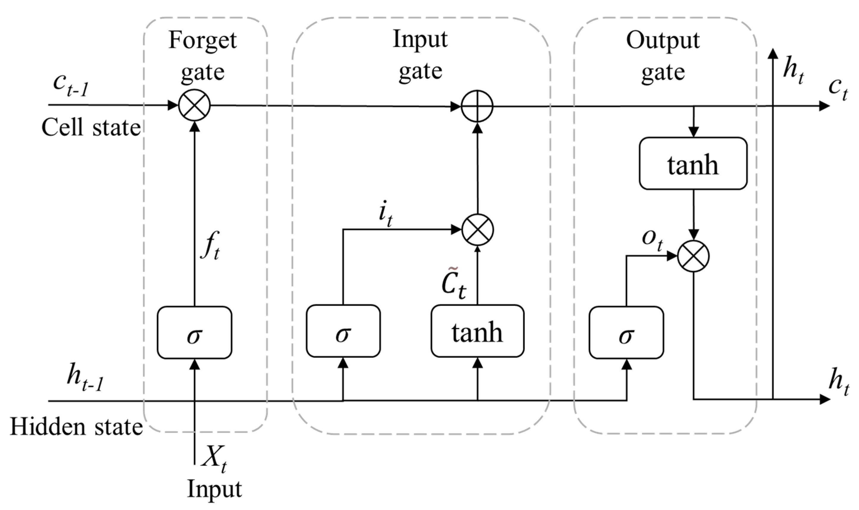
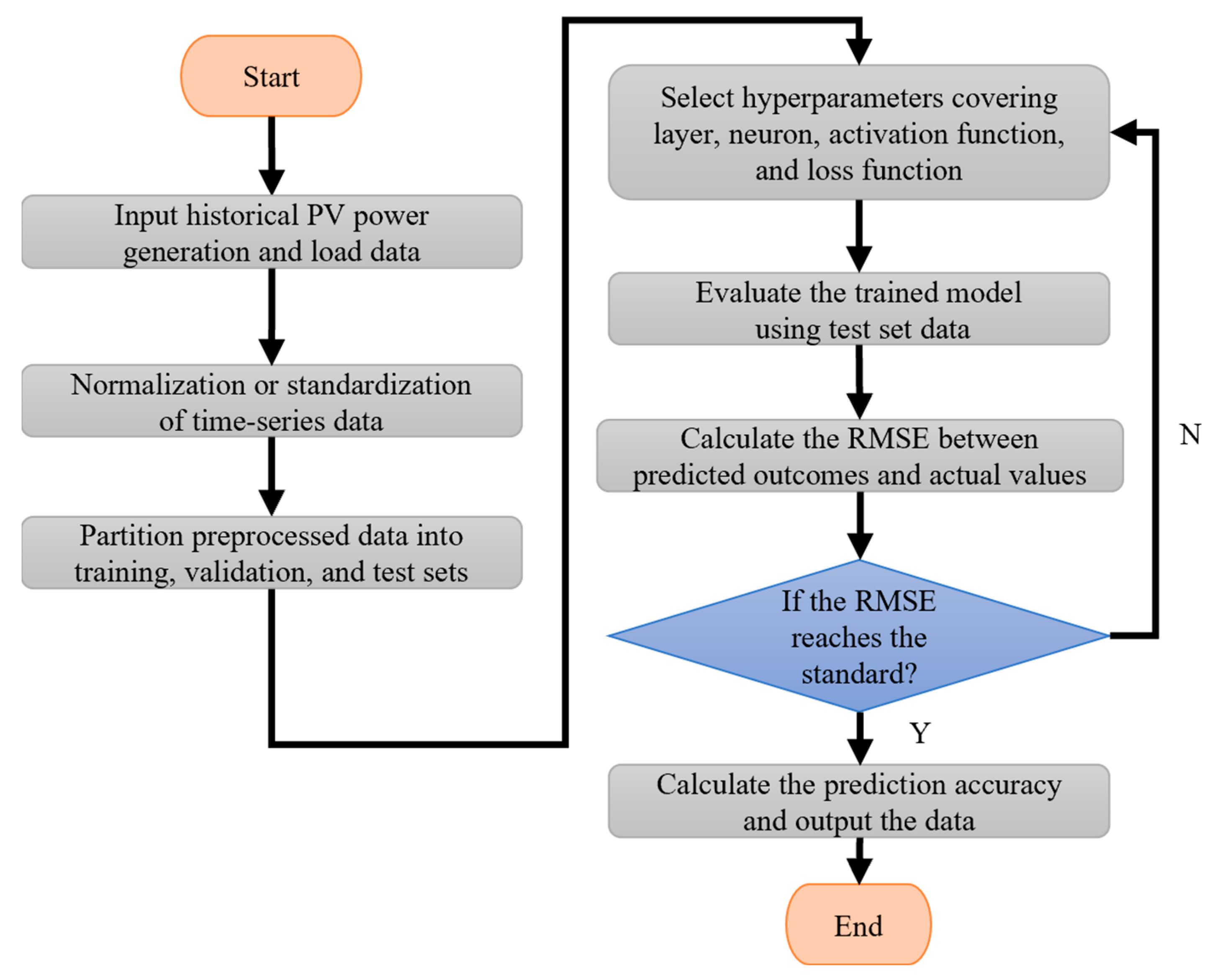
2.3. LSTM Neural Network-Based Prediction Model

PV power generation and load demand inherently exhibit volatility due to weather intermittency and load characteristics. The LSTM neural network is a gated recurrent architecture specifically designed to resolve the long-term dependency issues associated with conventional recurrent neural networks (RNNs) through its advanced gating mechanisms [26]. This architecture initiates operation via a gating mechanism that regulates information retention in the cell state, demonstrating resilience to non-stationary time series by dynamically adjusting memory retention through its gates. This eliminates the need for rigorous data differencing or normalization, which are often required due to data volatility. The first critical component, known as the forget gate, employs a sigmoid activation function to produce a vector of retention coefficients as described in Equation (10). This gate generates element-wise multiplicative weights that determine the retention ratio of each dimension in the preceding cell state, with values of 1 indicating complete retention and values of 0 representing complete elimination.

$$f_t=\sigma \cdot (W_f\cdot (X_t,h_{t-1})+b_f)$$

(10)

Here, h_t−1 denotes the previous hidden state, and X_t denotes the current input.

The subsequent information integration phase involves two parallel transformations within the input gate: a sigmoid-activated update gate and a hyperbolic tangent-activated candidate state generator, represented by Equation (11) and Equation (12), respectively. These components collectively determine both the update magnitude and the candidate state values. The cell state update is then updated through a composite operation, as formalized in Equation (13), where C_t−1 denotes the previous cell state.

$$i_t=\sigma \cdot (W_i\cdot (X_t,h_{t-1})+b_i)$$

(11)

$${\tilde{C}}_t=\tanh (W_C\cdot (X_t,h_{t-1})+b_c)$$

(12)

$$C_t=i_t\cdot {\tilde{C}}_t+f_t\cdot C_{t-1}$$

(13)

The final output gate regulates information exposure through a dual transformation process, as described by Equation (14) and Equation (15), respectively. This architecture ensures controlled propagation of long-term dependencies while maintaining gradient stability through the tanh-normalized exposure of the cell state. The resultant hidden state h_t serves as both the network output and the recurrent connection for subsequent time steps, thus preserving sequential dependencies across extended temporal intervals.

$$O_t=\sigma \cdot (W_o\cdot (X_t,h_{t-1})+b_0)$$

(14)

$$h_t=O_t\cdot \tanh (C_t)$$

(15)

The detailed architecture of a LSTM cell is illustrated in Figure 3. In this schematic diagram, X_t denotes the input vector at time step t, while h_t corresponds to the hidden state at the same time step. The rectangular blocks labeled with σ represent feedforward neural network layers employing the sigmoid activation function, which generate gating signals in the range [0, 1] to regulate information flow. Similarly, blocks labeled with tanh indicate feedforward layers utilizing the hyperbolic tangent activation function, generating candidate values in the range [−1, 1] for state updates.

The dimensionality of hidden neurons in these feedforward layers is determined through iterative training and validation processes involving systematic comparisons of prediction accuracy across multiple model configurations. This process ultimately identifies the optimal hyperparameter settings that maximize performance metrics such as sequence modeling capability and gradient stability. The gating mechanisms collectively enable fine control over long-range dependencies through element-wise multiplication and addition operations, effectively mitigating gradient vanishing issues that are commonly encountered in conventional RNN architectures.

The operational flowchart of the LSTM network is illustrated in Figure 4. Initially, the collected data undergo cleaning procedures, including handling missing values and outliers, followed by normalization or standardization to ensure appropriate value ranges for effective model training. Subsequently, the preprocessed data are partitioned into training, validation, and test sets according to predetermined ratios. The LSTM neural network architecture is then defined, specifying the number of layers, the number of neurons, and the activation functions, along with the selection of an appropriate optimizer and loss function. The model parameters are iteratively optimized using the training set, minimizing the loss function throughout the training process. Following this, the trained model is evaluated using test set data, and the root mean square error (RMSE) is calculated between predicted outcomes and actual values. If model performance is deemed unsatisfactory, hyperparameter adjustments are implemented until the standard of achieving an RMSE below 0.6 is met, ultimately yielding the final numerical predictions.

3. Solution Strategy

Given the presence of nonlinear terms in both the objective function and Equation (7), specific modifications are implemented to transform the original model into a linear one for the purpose of facilitating the solution process. Consequently, this study introduces the two variables F_ns and F_bs as follows:

$$F_{ns}=P_{n,t}\cdot stat{e}_{n,t}$$

(16)

$$F_{bs}=P_{b,t}\cdot stat{e}_{b,t}$$

(17)

By introducing the aforementioned variables F_ns and F_bs to replace the nonlinear terms in Equations (1) and (7), and simplifying accordingly, these equations can be rewritten as follows:

$$\min F_c=F_{pen}+{\displaystyle {\sum }_{t=1}^T[(C_{buy,t}-C_{sell,t})\cdot F_{ns,t}}+C_{sell,t}\cdot P_{ns,t}]\cdot \tau$$

(18)

$$SO{C}_t=SO{C}_{t-1}+[(1-{\displaystyle \frac{1}{\eta }})\cdot F_{bs,t}+{\displaystyle \frac{1}{\eta }}\cdot P_{b,t}]\cdot \tau /S_{bat}$$

(19)

Additionally, the following constraints are imposed:

$$-P_{n,\max }\cdot stat{e}_{n,t}\le F_{ns,t}\le P_{n,\max }\cdot stat{e}_{n,t}$$

(20)

$$P_{n,t}-P_{n,\max }\cdot (1-stat{e}_{n,t})\le F_{ns,t}\le P_{n,t}+P_{n,\max }\cdot (1-stat{e}_{n,t})$$

(21)

$$-P_{b,\max }\cdot stat{e}_{b,t}\le F_{bs,t}\le P_{b,\max }\cdot stat{e}_{b,t}$$

(22)

$$P_{b,t}-P_{b,\max }\cdot (1-stat{e}_{b,t})\le F_{bs,t}\le P_{b,t}+P_{b,\max }\cdot (1-stat{e}_{b,t})$$

(23)

The aforementioned constraints eliminate nonlinear terms within the mathematical model while maintaining strict equivalence to the original constraint definitions, thereby enabling the reformulation of the optimization model into a MILP model without compromising the physical or operational intent of the primal problem.

In summary, the following MILP model for the full-scale microgrid can be formulated as follows:

$$\min F_c=F_{pen}+{\displaystyle {\sum }_{t=1}^T[(C_{buy,t}-C_{sell,t})\cdot F_{ns,t}+C_{sell,t}\cdot P_{n,t}]}\cdot \tau$$

(24)

$$\mathrm{s}.\mathrm{t} \left\{\begin{array}{l}{F}_{pen}={\displaystyle {\sum }_{t=1}^T\left|stat{e}_{b,t}-stat{e}_{b,t-1}\right|}\cdot f_{pen}\\ P_{d,t}=P_{s,t}+P_{n,t}-P_{b,t}\\ 0\le P_{s,t}\le P_{s,\max }\\ -P_{n,\max }\cdot stat{e}_{b,t}+P_{n,\lim }\cdot (1-stat{e}_{b,t})\le P_{n,t}\le P_{n,\max }\\ -P_{b,\max }\le P_{b,t}\le P_{b,\max }\\ SO{C}_{\min }\le SO{C}_t\le SO{C}_{\max }\\ SO{C}_{start}=SO{C}_{end}\\ SO{C}_t=SO{C}_{t-1}+[(1-{\displaystyle \frac{1}{\eta }})\cdot F_{bs,t}+{\displaystyle \frac{1}{\eta }}\cdot P_{b,t}]\cdot \tau /S_{bat}\\ -P_{n,\max }\cdot stat{e}_{n,t}\le F_{ns,t}\le P_{n,\max }\cdot stat{e}_{n,t}\\ P_{n,t}-P_{n,\max }\cdot (1-stat{e}_{n,t})\le F_{ns,t}\le P_{n,t}+P_{n,\max }\cdot (1-stat{e}_{n,t})\\ -P_{b,\max }\cdot stat{e}_{b,t}\le F_{bs,t}\le P_{b,\max }\cdot stat{e}_{b,t}\\ P_{b,t}-P_{b,\max }\cdot (1-stat{e}_{b,t})\le F_{bs,t}\le P_{b,t}+P_{b,\max }\cdot (1-stat{e}_{b,t})\end{array}\right.$$

(25)

The aforementioned model can be solved using the Gurobi 11.0.1 solver, which is manufactured by Gurobi Optimization LLC, located in Houston, Texas, United States, within MATLAB^TM R2023b. The day-ahead optimal scheduling framework proposed in this paper for the full-scale microgrid comprises three main stages: (1) forecasting PV power generation and load demand under various weather conditions using the LSTM neural network; (2) formulating and solving the day-ahead optimal scheduling model to determine the optimal scheduling strategy; and (3) validating the proposed strategy through field experiments in the full-scale microgrid under various weather conditions. The solution flowchart is presented in Figure 5, and the corresponding specific steps are described as follows:

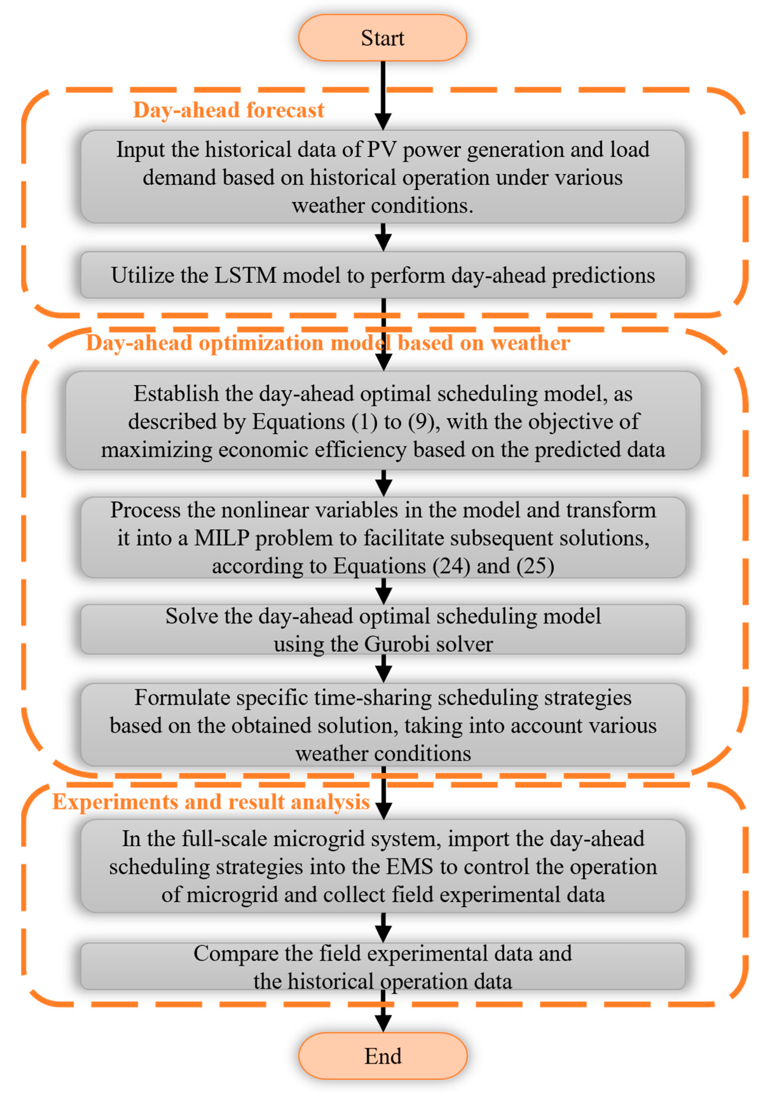
• Input the historical data of PV power generation and load demand into the model, based on historical operation under various weather conditions.
• Utilize the LSTM neural network to perform day-ahead predictions of PV power generation and load demand for the microgrid under various weather conditions.
• Establish the day-ahead optimal scheduling model, as described by Equation (1) to (9), with the objective of maximizing economic efficiency based on the predicted data.
• Process the nonlinear variables in the model and transform it into a MILP problem to facilitate subsequent solutions, according to Equations (24) and (25).
• Solve the day-ahead optimal scheduling model of the microgrid in MATLAB using the Gurobi solver.
• Formulate specific time-sharing scheduling strategies for the microgrid throughout the day based on the obtained solution, taking into account various weather conditions.
• In the full-scale microgrid system, import the corresponding day-ahead scheduling strategies, tailored to the identified weather conditions, into the EMS to control the operation of the microgrid and collect field experimental data.
• Compare the field experimental data with historical operational data to assess the effectiveness of the proposed scheduling strategies.

4. Case Study

To validate the effectiveness of the proposed optimal scheduling, a case study is performed on a full-scale microgrid system deployed within an industrial park located in Shenzhen. The configuration parameters of the microgrid are initially introduced, including details regarding time-of-use electricity prices. Subsequently, the LSTM neural network is employed to forecast PV power generation and industrial load demand under both sunny and cloudy weather conditions. Simulations are carried out under these two distinct scenarios, highlighting the variability in energy output and demand that the microgrid may experience. Finally, the full-scale microgrid is utilized to conduct field experimental validation of the simulation results.

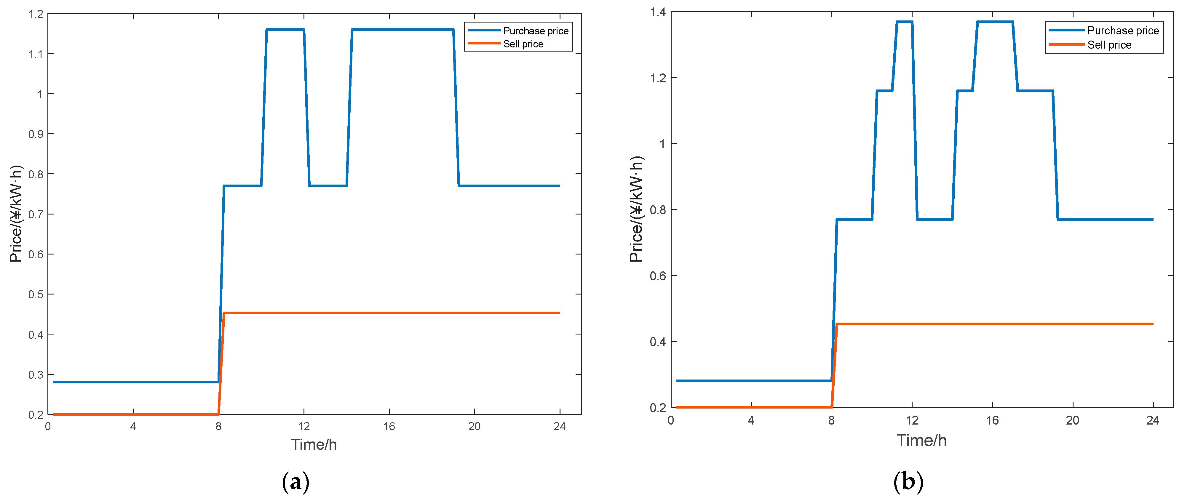
4.1. Configuration Parameters

In this study, a mathematical model is developed in MATLAB^TM for a full-scale grid-connected PV–energy storage microgrid within a specific industrial park in Shenzhen. The model includes two operational scenarios: cloudy and sunny days. The microgrid components include a PV power generation system, an energy storage battery system, the regular load of the park, and the machining load. The maximum power generation capacity of the PV system is 78.00 kW, while the rated capacity of the energy storage battery is 200.00 kWh, with a maximum charging and discharging power of 68.00 kW and a charging and discharging efficiency of 86.00%. The maximum exchange power between the microgrid and the main power grid is 70.00 kW, and the SOC of the battery has a maximum and minimum of 100.00% and 4.80%, respectively. The time-of-use electricity prices for purchasing and selling electricity in Shenzhen are shown in Figure 6, which indicates that the time-of-use electricity prices for July and August also include peak electricity rates. The selling price is uniformly set at 0.45 CNY/kWh for all periods except during 0:00–8:00.

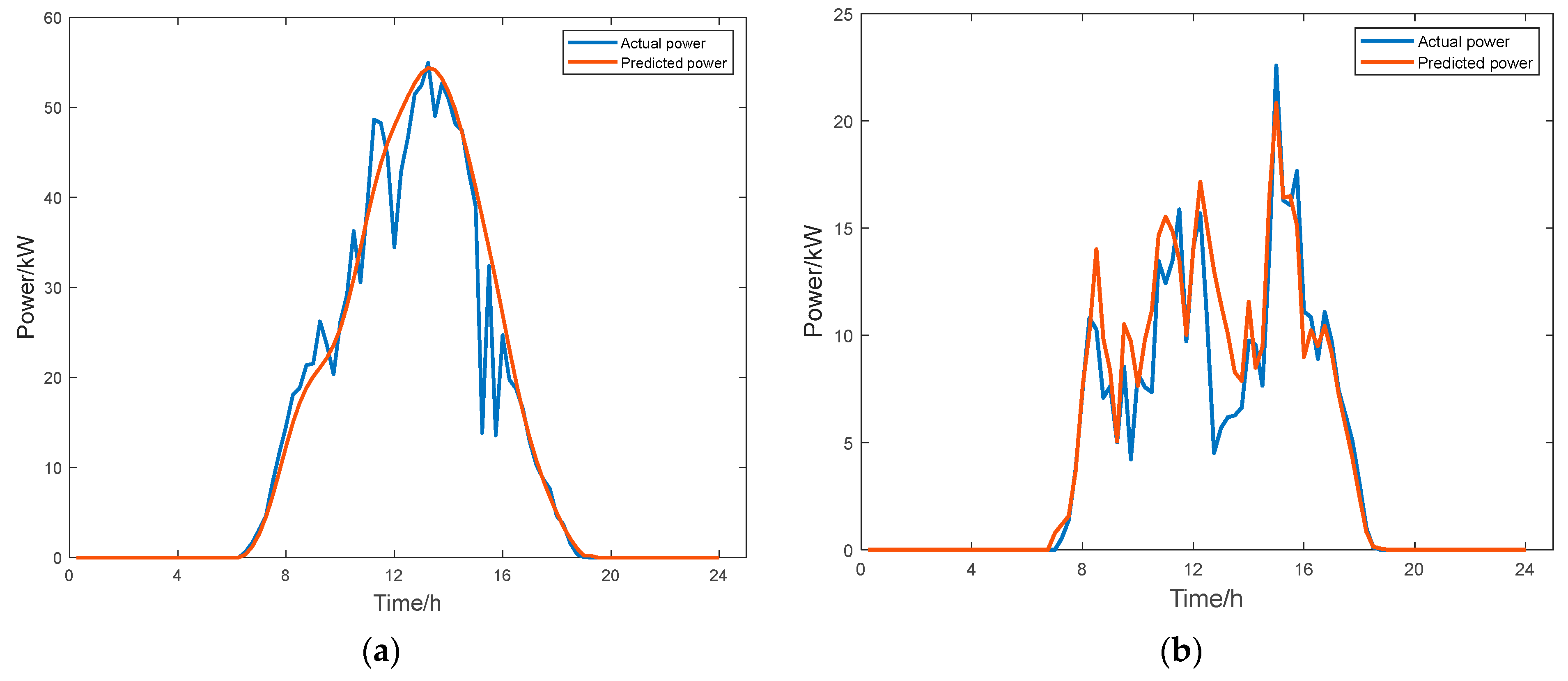
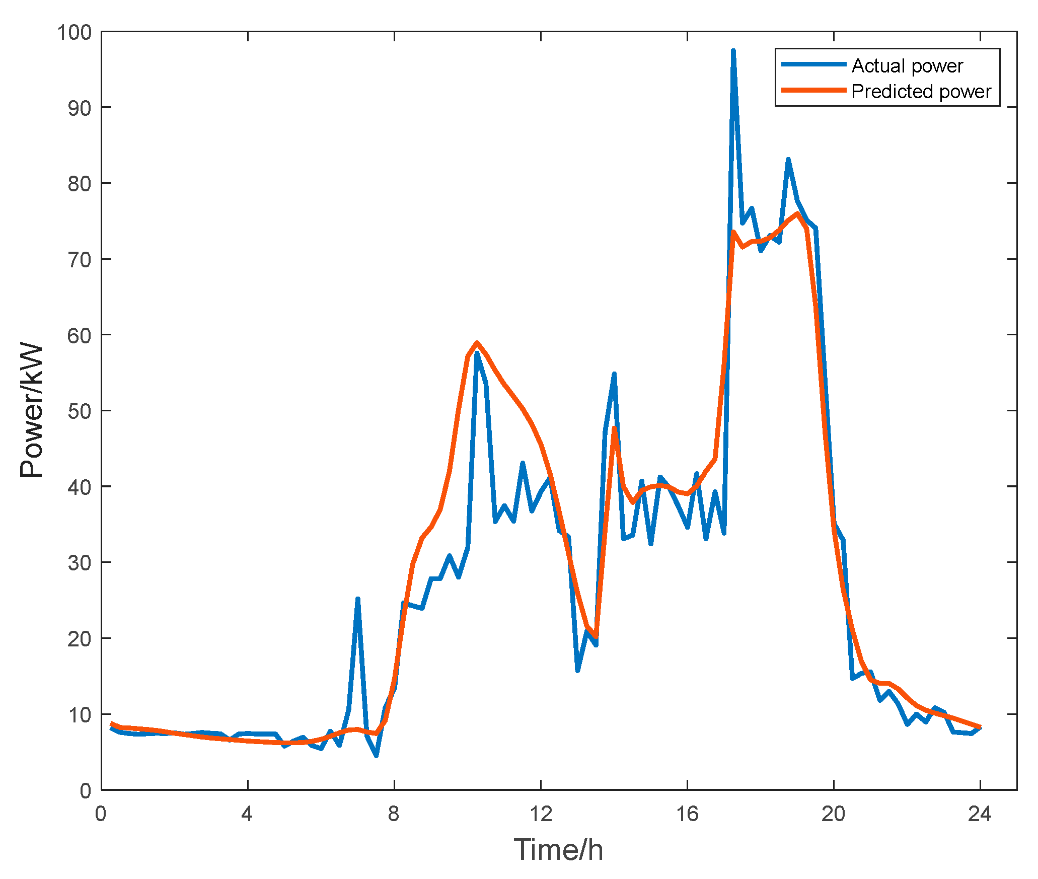
4.2. Forecasting Results for PV Power Generation and Load Demand

Based on the actual PV power generation data collected on both sunny and cloudy days, along with the load data from the microgrid, an LSTM neural network based on a prediction model is developed. The LSTM model is configured with 200 hidden layer units, a learning rate of 0.005, and a maximum of 1000 iterations. It employs a piecewise learning rate decay strategy with a decay interval of 125 epochs and a dropout rate of 0.2. The comparison curves of the predicted data against the actual data from subsequent field experiments are shown in Figure 7 and Figure 8, respectively. The prediction accuracy is calculated under the assumption that the relative error remains within 20.00%, indicating that the predicted values are acceptable. The results indicate that the prediction accuracy for PV power generation on sunny days is 75.00%, with a RMSE of 0.28. For cloudy days, the accuracy is 67.39%, with a RMSE of 0.52, while the prediction accuracy for the load demand is 78.12%, yielding a RMSE of 0.34. Overall, the trend of the predicted result curves closely aligns with that of the actual curves.

4.3. Simulation Analysis

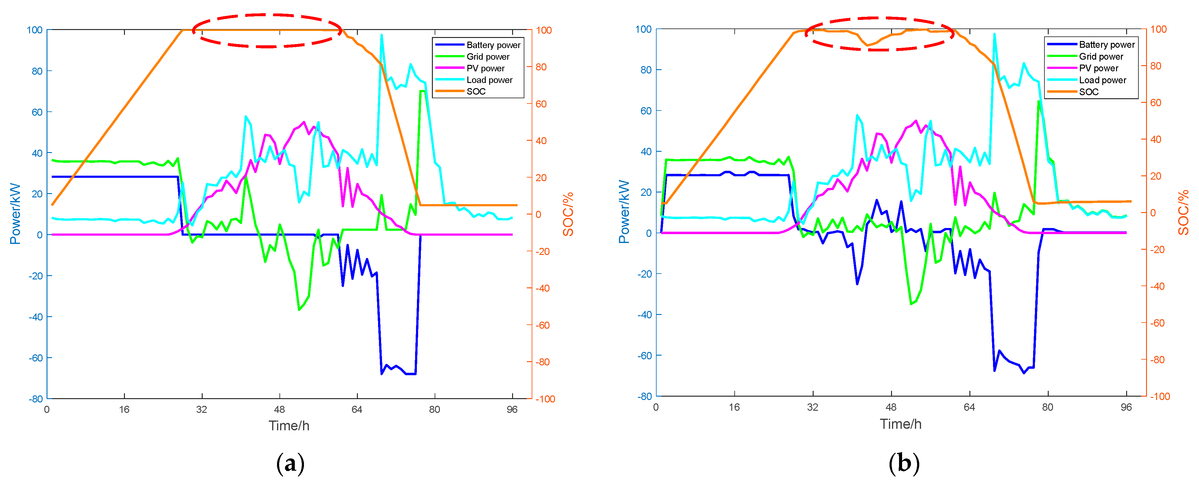
4.3.1. Sunny Day Scenario

The PV power generation and load data for sunny days, obtained from the LSTM neural network based on the prediction model, are utilized as input and substituted into the optimization model for analysis. Subsequently, a comparative analysis is performed against the historical data from the actual operational mode of the full-scale microgrid. The time interval for the optimization model is set to τ = 0.25 h. The state curve of the microgrid following optimization is shown in Figure 9.

After optimization, the system actively employs energy storage to supply the load between 8:00 and 15:00. During this period, surplus PV power is utilized to charge the batteries, while the operational mode at other times remains consistent with that of the historical operational state. The key differences between the optimized results and the original operating mode are highlighted with a red dashed circle.

In the historical operational state, the daily operating cost of the microgrid is CNY 190.03. Following optimization, the daily operating cost decreases to CNY 180.69, resulting in a reduction in operating expenses of 4.92% following the optimization. Additionally, the fluctuations in the grid-connected power of the microgrid were mitigated, resulting in enhanced system stability.

4.3.2. Cloudy Day Scenario

Similarly, the PV power generation and load data for cloudy days, obtained from the LSTM prediction model, are utilized as input and substituted into the optimization model for analysis. The time interval of the optimization model is set to τ = 0.25 h. The state curve of the microgrid following optimization is shown in Figure 10. The key differences between the optimized results and the original operating mode are highlighted with a red dashed circle.

After optimization, the system employs power from the energy storage battery to supply the load from 10:00 to 14:00. Concurrently, a portion of the main grid power is utilized to charge the battery, while the operational mode during other times remains consistent with that of the historical operational state.

In the historical operational mode, the daily operating cost of the microgrid is CNY 385.69. Following optimization, this cost is reduced to CNY 375.07, resulting in a reduction in operating expenses of 2.75% following the optimization.

From an annual perspective, according to the weather data of Shenzhen in 2023 [27], the city experienced a total of 258 sunny days and 107 rainy or cloudy days. This includes 28 sunny days and 34 rainy or cloudy days during July and August, the months characterized by peak electricity prices. In addition, it is important to exclude instances of extremely low loads occurring on Sundays and holidays, which constitute approximately one-seventh of the entire year. It is estimated that there are approximately 221 sunny days and 92 rainy or cloudy days on non-holidays in Shenzhen each year; specifically, in July and August, there are around 24 sunny days and 30 rainy or cloudy days.

According to the solution of the proposed optimization model, under the sunny scenarios in July and August, the daily operating cost prior to optimization is CNY 192.06, which is reduced to CNY 182.06 after optimization. Under the rainy or cloudy scenarios, the daily operating cost prior to optimization is CNY 394.23, decreasing to CNY 376.59 after optimization. Consequently, the estimated annual operating cost prior to optimization totals CNY 77,785.03, while the cost after optimization amounts to CNY 74,517.41. This yields total annual savings of CNY 3267.62, corresponding to a cost savings ratio of 4.20% compared to the previous situation.

Table 1. Historical operating costs and operating costs after simulation optimization.

	Historical Operating Costs	Operating Costs After Simulation Optimization	Cost Savings
Sunny day (excluding the months of July and August)	CNY 190.03	CNY 180.69	CNY 9.34
Cloudy day (excluding the months of July and August)	CNY 385.69	CNY 375.07	CNY 10.62
Sunny day (during the months of July and August)	CNY 192.06	CNY 182.06	CNY 10.00
Cloudy day (during the months of July and August)	CNY 394.23	CNY 376.59	CNY 17.64
The entire year (estimated)	CNY 77,785.03	CNY 74,517.41	CNY 3267.62

presents the statistical results of the operating costs of the microgrid before and after simulation optimization under various weather conditions described above.

5. Experimental Validation

5.1. Experimental Scheme

Based on the optimization curves discussed above, the field experimental schemes for the microgrid under sunny and cloudy weather conditions are formulated as follows:

Sunny scenario:

• From 0:00 to 8:00, the energy storage battery is charged at a designated power level until it reaches the maximum SOC.
• From 8:00 to 15:00, the energy storage battery and PV power jointly supply the system load, with any surplus power from the PV system used to charge the battery.
• From 15:00 to 24:00, the energy storage battery and PV power continue to jointly supply the system load. If power is insufficient, additional power will be sourced from the main grid.

Cloudy scenario:

• From 0:00 to 8:00, the energy storage battery is charged at a designated power level until it reaches the maximum SOC.
• From 8:00 to 10:00, the power grid and PV power jointly supply the system load while the energy storage battery remains inactive.
• From 10:00 to 12:00, the energy storage battery and PV power work together to supply the load.
• From 12:00 to 14:00, the main power grid supplies power to the microgrid at its maximum capacity. A portion of this power is utilized to jointly supply the load alongside the PV system, while the remainder charges the energy storage battery.
• From 14:00 to 24:00, the energy storage battery and PV power jointly supply the system load. If additional power is required, it will be sourced from the main grid.

5.2. Experimental Environment

The field experimental subject is the PV–energy storage microgrid located in a specific industrial park in Shenzhen. A photograph of the site is presented in Figure 11. The full-scale microgrid comprises PV panels, PV inverters, energy storage battery systems, and other components, all connected to the main power grid via a grid-connected transformer. The entire system is managed by the microgrid EMS. The meanings of the Chinese words in the right part of the EMS image from top to bottom are as follows: battery stack, energy storage meter, auxiliary meter, reverse current and overload protection meter, air conditioner.

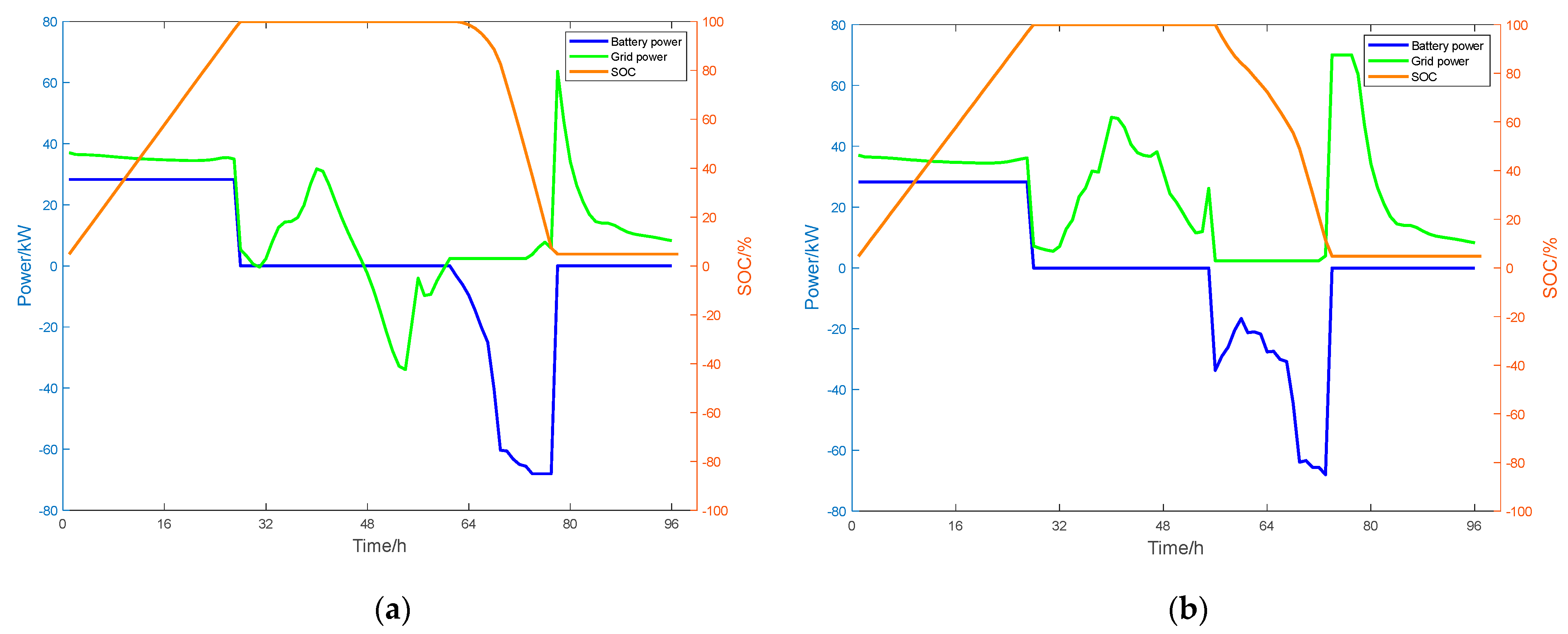
5.3. Field Experimental Results and Comparative Analysis

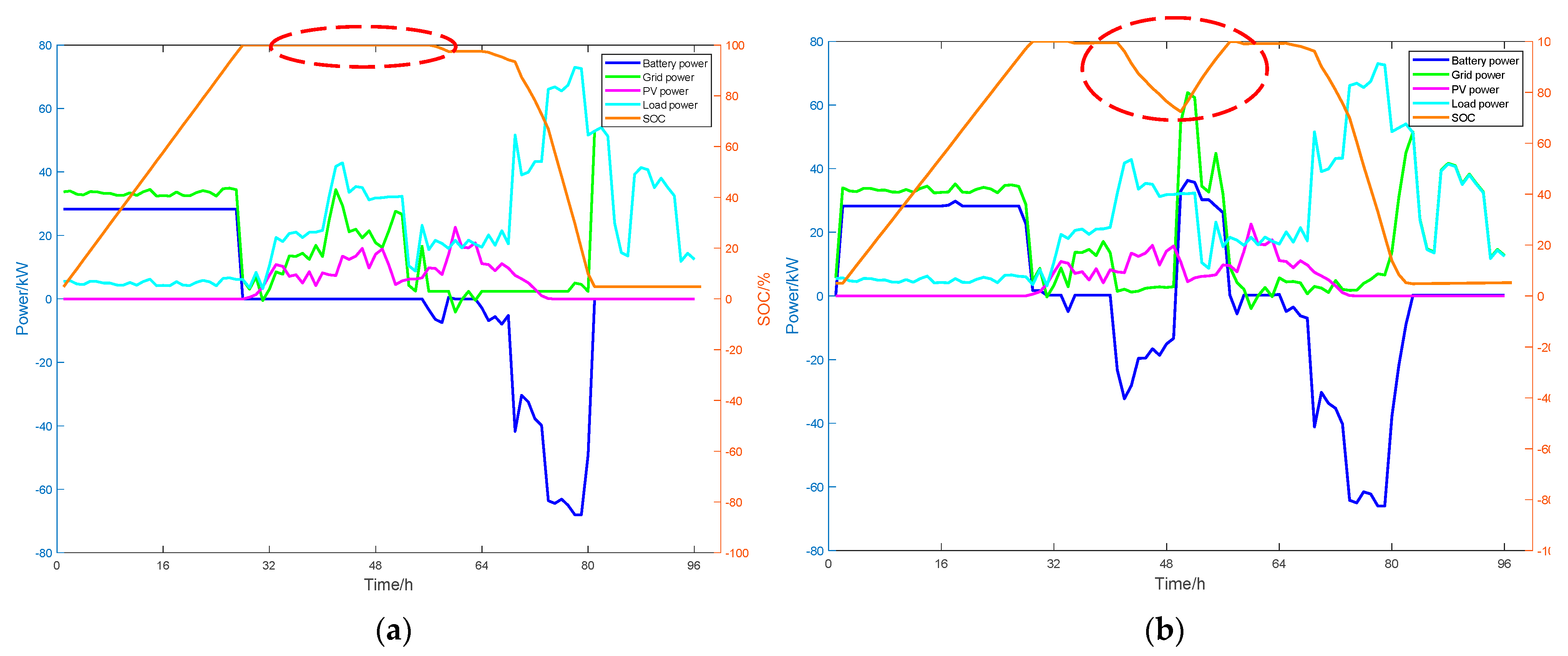
5.3.1. Field Experiments Under Sunny Day

On 3 September 2024, a sunny day, the energy storage system of the microgrid is operated according to the proposed field experimental scheme. The operational results are shown in Figure 12, which includes both the simulated operation curves based on the historical scheme and the actual operation curves under the field experimental scheme. The key differences between the original operating mode and the experimental results are highlighted with a red dashed circle respectively.

The results demonstrate that, under the PV power and load conditions of that day, the daily operating cost using the historical scheme is CNY 172.96, while the daily operating cost under the field experimental scheme is CNY 164.59, reflecting a cost reduction of 4.84%.

5.3.2. Field Experiments Under Cloudy Day

On 24 September 2024, a cloudy day, the energy storage system is similarly scheduled according to the field experimental scheme, with the operational results depicted in Figure 13. This figure shows the simulated operation curves based on the historical scheme alongside the actual results from the field experimental scheme. The key differences between the original operating mode and the experimental results are highlighted with a red dashed circle respectively.

The findings indicate that under the day’s PV power and load conditions, the daily operating cost with the historical scheme is CNY 273.86 and CNY 266.88 with the field experimental scheme, resulting in a cost reduction of 2.55%.

For sunny days in July and August, the daily operating cost prior to optimization is CNY 174.23 compared to CNY 166.50 after optimization. For rainy and cloudy days, the cost prior to optimization is CNY 278.84, while after optimization, it is CNY 268.60. Based on the weather data for Shenzhen in 2023, the approximate annual operating cost prior to optimization is CNY 63,599.16, and after optimization, it is CNY 61,024.79, yielding total annual savings of CNY 2574.37 and a cost savings ratio of 4.05% compared to the previous situation.

Table 2. Historical operating costs and experimental operating costs after optimization.

	Historical Operating Costs	Operating Costs under the Experimental Scheme	Cost Savings
Sunny day (excluding the months of July and August)	CNY 172.96	CNY 164.59	CNY 8.37
Cloudy day (excluding the months of July and August)	CNY 273.86	CNY 266.88	CNY 6.98
Sunny day (during the months of July and August)	CNY 174.23	CNY 166.50	CNY 7.73
Cloudy day (during the months of July and August)	CNY 278.84	CNY 268.60	CNY 10.24
The entire year (estimated)	CNY 63,599.16	CNY 61,024.79	CNY 2574.37

presents the statistical results of the operating costs of the microgrid under the field experimental scheme described above.

The construction cost of the PV system in this full-scale microgrid is approximately CNY 250,000.00, while the energy storage system costs around CNY 260,000.00, resulting in a total construction cost of roughly CNY 510,000.00. Prior to the construction of the PV and energy storage systems, the operating costs under different conditions are as follows: excluding July and August, the cost on sunny days is CNY 602.12, which increases to CNY 626.04 during July and August. Similarly, for cloudy days, the cost is CNY 493.14 excluding July and August, and it increases to CNY 507.88 during these months. Based on annual data calculations, the annual operating cost before the construction of the PV and energy storage systems is CNY 179,453.68. By comparing the total construction cost with the original operational plan, the payback period is estimated to be approximately 4.40 years. Under the optimized operational plan, this period is reduced to 4.30 years, thereby shortening the payback period by about 36 days.

In addition, a comparison of the simulation results with the field experimental outcomes reveals that the decrease in daily operating costs from the field experimental results is less pronounced than that observed in the simulation results. The reasons for this discrepancy are as follows:

• Variability in the accuracy of PV power generation and load demand predictions led to discrepancies between the actual conditions observed during the field experiments and the predicted values, resulting in certain operational errors.
• While the simulation results allow real-time adjustments according to current PV power generation and load demand, the day-ahead scheduling model does not permit changes to the operational strategy in response to real-time monitoring of the current conditions, leading to suboptimal outcomes.

6. Conclusions

This study proposes an optimization model designed to minimize the total daily operating cost of a full-scale PV–energy storage microgrid system. Leveraging historical operational data from the microgrid, short-term predictions of PV power generation and load demand are performed for day-ahead scheduling, upon which the established optimization model is solved. Through simulation analysis and field experimental validation conducted on the full-scale microgrid, the feasibility and effectiveness of the proposed optimal scheduling scheme are demonstrated. The simulation and field experimental results indicate that, under the proposed optimal scheduling scheme, the daily operating cost of the microgrid can be reduced by 4.84% and 2.55% under sunny and cloudy weather conditions, respectively. The optimal scheduling strategy proposed in this study offers significant guidance and reference value for the safe and economical operation of current PV–energy storage microgrids. Future research could enhance the model by integrating more accurate prediction methods. Additionally, adopting a rolling prediction approach could facilitate real-time adjustments to the operational strategy according to current conditions, thereby enhancing the effectiveness of the strategy. In addition, the optimal operation of microgrids considering security and the potential impact of cyber attacks should also be discussed in future studies.

References

1. Zhang, X.; Wang, C.; Xie, K.; Li, Q.; Zhang, N.; Wu, S. Key Issues in the Construction of China’s Green Power Market under the “Carbon Peaking and Carbon Neutrality” Goals. Autom. Electr. Power Syst. 2024, 48, 25–33. (In Chinese) [Google Scholar] [CrossRef]
2. Akinyele, D.; Belikov, J.; Levron, Y. Challenges of Microgrids in Remote Communities: A STEEP Model Application. Energies 2018, 11, 432. [Google Scholar] [CrossRef]
3. Li, Y.; Zhang, F.; Li, Y.; Wang, Y. An Improved Two-Stage Robust Optimization Model for CCHP-P2G Microgrid System Considering Multi-Energy Operation under Wind Power Outputs Uncertainties. Energy 2021, 223, 120048. [Google Scholar] [CrossRef]
4. Wang, W.; Yuan, B.; Sun, Q.; Wennersten, R. Application of Energy Storage in Integrated Energy Systems—A Solution to Fluctuation and Uncertainty of Renewable Energy. J. Energy Storage 2022, 52, 104812. [Google Scholar] [CrossRef]
5. Priolkar, J.; ES, S. Distributed Generation and Demand Response Coordination for Optimal Operation of Microgrid Using Modified Elephant Herd Optimization. Electr. Power Compon. Syst. 2024, 1–18. [Google Scholar] [CrossRef]
6. Armghan, H.; Xu, Y.; Ali, N.; Farooq, U. Coordination Control in Hybrid Energy Storage Based Microgrids Providing Ancillary Services: A Three-Layer Control Approach. J. Energy Storage 2024, 93, 112221. [Google Scholar] [CrossRef]
7. Dini, A.; Hassankashi, A.; Pirouzi, S.; Lehtonen, M.; Arandian, B.; Baziar, A.A. A Flexible-Reliable Operation Optimization Model of the Networked Energy Hubs with Distributed Generations, Energy Storage Systems and Demand Response. Energy 2022, 239, 121923. [Google Scholar] [CrossRef]
8. Rawa, M.; Al-Turki, Y.; Sedraoui, K.; Dadfar, S.; Khaki, M. Optimal Operation and Stochastic Scheduling of Renewable Energy of a Microgrid with Optimal Sizing of Battery Energy Storage Considering Cost Reduction. J. Energy Storage 2023, 59, 106475. [Google Scholar] [CrossRef]
9. Chakraborty, A.; Ray, S. Economic and Environmental Factors based Multi-Objective Approach for Optimizing Energy Management in a Microgrid. Renew. Energy 2024, 222, 119920. [Google Scholar] [CrossRef]
10. Dey, B.; Misra, S.; Marquez FP, G. Microgrid System Energy Management with Demand Response Program for Clean and Economical Operation. Appl. Energy 2023, 334, 120717. [Google Scholar] [CrossRef]
11. Sun, L.; Ding, D.; Dong, H.; Yi, X. Distributed Economic Dispatch of Microgrids Based on ADMM Algorithms with Encryption-Decryption Rules. IEEE Trans. Autom. Sci. Eng. 2025, 22, 8427–8438. [Google Scholar] [CrossRef]
12. Zhang, H.; Yue, D.; Dou, C.; Hancke, G.P. PBI Based Multi-Objective Optimization via Deep Reinforcement Elite Learning Strategy for Micro-grid Dispatch with Frequency Dynamics. IEEE Trans. Power Syst. 2022, 38, 488–498. [Google Scholar] [CrossRef]
13. Zhang, H.; Qin, W.; Han, X.; Wang, P.; Guo, X. Optimization Scheduling Scheme for Energy Management of Microgrid in Multiple Time Scales. Power Syst. Technol. 2017, 41, 1533–1542. (In Chinese) [Google Scholar] [CrossRef]
14. Ponnambalam, K.; Quintana, V.; Vannelli, A. A Fast Algorithm for Power System Optimization Problems Using an Interior Point Method. IEEE Trans. Power Syst. 1992, 7, 892–899. [Google Scholar] [CrossRef]
15. Zhu, P.; Liu, Z.; Sun, K.; Wang, L.; Hu, P.; Zhu, N.; Jiang, D. Distributed Model Predictive Control Strategy Based on Block-Wised Alternating Direction Multiplier Method for Microgrid Clusters. IET Gener. Transm. Distrib. 2022, 16, 4630–4639. [Google Scholar] [CrossRef]
16. Kölsch, L.; Wieninger, K.; Krebs, S.; Hohmann, S. Distributed Frequency and Voltage Control for AC Microgrids Based on Primal-Dual Gradient Dynamics. IFAC PapersOnLine 2020, 53, 12229–12236. [Google Scholar] [CrossRef]
17. Huangfu, Y.; Tian, C.; Zhuo, S.; Xu, L.; Li, P.; Quan, S.; Zhang, Y.; Ma, R. An Optimal Energy Management Strategy with Subsection Bi-Objective Optimization Dynamic Programming for Photovoltaic/Battery/Hydrogen Hybrid Energy System. Int. J. Hydrogen Energy 2023, 48, 3154–3170. [Google Scholar] [CrossRef]
18. Feng, Y.; Hu, D. Research on Optimal Scheduling of Grid-Connected Microgrid Based on Simulated Annealing Genetic Algorithm. Electr. Eng. Mater. 2022, 183, 75–80. (In Chinese) [Google Scholar] [CrossRef]
19. Park, J.-B.; Jeong, Y.-W.; Shin, J.-R.; Lee, K.Y. An Improved Particle Swarm Optimization for Nonconvex Economic Dispatch Problems. IEEE Trans. Power Syst. 2010, 25, 156–166. [Google Scholar] [CrossRef]
20. Khatod, D.; Pant, V.; Sharma, J. Evolutionary Programming Based Optimal Placement of Renewable Distributed Generators. IEEE Trans. Power Syst. 2013, 28, 683–695. [Google Scholar] [CrossRef]
21. Abdollahzadeh, B.; Gharehchopogh, F.S.; Khodadadi, N.; Mirjalili, S. Mountain Gazelle Optimizer: A New Nature-Inspired Metaheuristic Algorithm for Global Optimization Problems. Adv. Eng. Softw. 2022, 174, 103282. [Google Scholar] [CrossRef]
22. Zuo, F.; Zhang, Y.; Zhao, Q.; Sun, L. Two-Stage Stochastic Optimization for Operation Scheduling and Capacity Allocation of Integrated Energy Production Unit Considering Supply and Demand Uncertainty. Proc. CSEE 2022, 42, 8205–8215. (In Chinese) [Google Scholar] [CrossRef]
23. Sun, P.; Teng, Y.; Hui, Q.; Chen, Z. Two-Stage Robust Optimal Scheduling Model for Multi-Energy Systems Considering Thermal Inertia Uncertainty. Proc. CSEE 2021, 41, 7249–7260. (In Chinese) [Google Scholar] [CrossRef]
24. Aaslid, P.; Korpas, M.; Belsnes, M.M.; Fosso, O.B. Stochastic Optimization of Microgrid Operation with Renewable Generation and Energy Storages. IEEE Trans. Sustain. Energy 2022, 13, 1481–1491. [Google Scholar] [CrossRef]
25. Hematian, H.; Askari, M.T.; Ahmadi, M.A.; Sameemoqadam, M.; Nik, M.B. Robust Optimization for Microgrid Management with Compensator, EV, Storage, Demand Response, and Renewable Integration. IEEE Access 2024, 12, 73413–73425. [Google Scholar] [CrossRef]
26. Campos, F.; Sousa, T.; Barbosa, R. Short-Term Forecast of Photovoltaic Solar Energy Production Using LSTM. Energies 2024, 17, 2582. [Google Scholar] [CrossRef]
27. Shenzhen Climate Bulletin (2023). Shenzhen Special Zone Daily (A08), 29 January 2023. [CrossRef]
Figure 1. Schematic diagram of the microgrid.
Electronics 14 01509 g001
Figure 2. (a) SOC profiles of energy storage systems and microgrid power variations under sunny weather conditions; (b) SOC profiles of energy storage systems and microgrid power variations under cloudy weather conditions.
Electronics 14 01509 g002
Figure 3. Architecture of a LSTM cell.
Electronics 14 01509 g003
Figure 4. Flowchart of the LSTM neural network for forecasting PV power generation and load demand.
Electronics 14 01509 g004
Figure 5. Solution flowchart for the day-ahead optimal scheduling model of the microgrid.
Electronics 14 01509 g005
Figure 6. (a) Time-of-use electricity prices for purchasing and selling electricity in Shenzhen, excluding the months of July and August; (b) time-of-use electricity prices for purchasing and selling electricity in Shenzhen during the months of July and August.
Electronics 14 01509 g006
Figure 7. (a) Comparison curves of PV power generation prediction results versus actual data on sunny days; (b) comparison curves of PV power generation prediction results versus actual data on cloudy days.
Electronics 14 01509 g007
Figure 8. Comparison curves of the load prediction result curve versus the actual data curve.
Electronics 14 01509 g008
Figure 9. Curves of energy storage SOC and microgrid power variation in a sunny scenario following optimization.
Electronics 14 01509 g009
Figure 10. Curves of energy storage SOC and microgrid power variation in a cloudy scenario following optimization.
Electronics 14 01509 g010
Figure 11. Schematic diagram of the full-scale PV–energy storage microgrid.
Electronics 14 01509 g011
Figure 12. (a) Curves of the full-scale microgrid energy storage SOC and power variation before optimization during a sunny day; (b) curves of the full-scale microgrid energy storage SOC and power variation after optimization during a sunny day.
Electronics 14 01509 g012
Figure 13. (a) Curves of the full-scale microgrid energy storage SOC and power variation before optimization during a cloudy day; (b) curves of the full-scale microgrid energy storage SOC and power variation after optimization during a cloudy day.
Electronics 14 01509 g013