Vehicle Height Lifting Strategy Based on Double-Vector Control of Permanent Magnet Synchronous Linear Motor

Abstract

Conventional active vehicle height control systems predominantly employ hydraulic or pneumatic suspension mechanisms. Although these established approaches have achieved widespread adoption in automotive applications, they remain fundamentally constrained by three critical drawbacks: (1) inadequate dynamic response characteristics, (2) high energy consumption, and (3) inherent mechanical complexity. The ongoing electrification revolution in vehicle technologies has spurred significant research interest in linear electromagnetic suspension systems. Nevertheless, their practical implementation encounters dual technical barriers: (a) complex multi-phase motor configurations requiring precise coordination, and (b) substantial thrust ripple generation under dynamic operating conditions. To address these critical limitations, our research proposes a novel motor structure, known as the flat rectangular slot structure, which offers advantages such as simple installation and high thrust with low current. Additionally, we have designed a double-vector control strategy for the motor control section, which modifies the finite-set model predictive control and enhances the accuracy of the model’s calculations. By integrating the vehicle model, we have developed a multi-layer hierarchical control strategy for the vehicle height controller. In the first layer, a PI controller is used to convert the target height into current, which is then input into the value function. In the second layer, we improve the control strategy for the linear motor by optimizing the finite-set model predictive control through the double-vector control. Through multi-step predictive calculations, we determine the optimal sector, enabling the motor to receive the corresponding control force. In the third layer, the motor thrust is input into the vehicle model to achieve closed-loop control of the vehicle body. Finally, we conduct simulation verification of the proposed control strategy. The simulation results indicate that the double-vector control significantly reduces the fluctuation in the sprung mass displacement by approximately 70% compared to single-vector control, the response speed is increased by approximately 20%, and the thrust required to achieve the target vehicle height is reduced by 5.7%. Therefore, the proposed double-vector control strategy can significantly enhance the stability of the automotive electronic control suspension, opening up new research avenues for the study of suspension stability control and energy saving in vehicles.

1. Introduction

Active suspension systems, represented by air suspension and hydraulic suspension, have gained increasing popularity among automotive manufacturers and consumers due to their wide adjustment range, fast response speed, and high ride comfort. However, these systems also have drawbacks, such as high sealing requirements and energy consumption, particularly exhibiting slow response during vehicle lift and lower control. In recent years, linear motors have emerged as a promising actuator technology, offering advantages such as rapid response speed, high adjustment accuracy, and stable force output [1,2,3]. This has gradually attracted the attention of researchers and automotive manufacturers. Currently, linear motors are widely used to improve the ride smoothness of vehicles. However, due to fluctuations in the thrust of linear motors and limitations of control algorithms, it is rare to see the research of linear motors applied to vehicle height control.

To address the improvement in electromagnetic thrust fluctuations and enhance the performance of electromagnetic thrust [4,5], some experts and scholars have approached the issue through structural design. Li Jing et al. [6] proposed a modular permanent magnet linear synchronous motor structure with 16 poles and 18 slots, introducing a new end tooth design that enhances the average thrust. Lan, Zhiyong [7] proposed a V-shaped tooth–slot structure to suppress and reduce electromagnetic thrust fluctuations in PMLSMs; the coil structure is also changed from rectangular to V-shaped coils meeting the same angle as the V-shaped tooth–slot. Meanwhile, the specific slot design is implemented using the infinitesimal method. Fu, Dongshan et al. [8] proposed a structurally simple novel flux-switching transverse flux linear motor. The results indicated that this method effectively reduced cogging force and improved thrust. Seal, Monojit et al. [9] improved a four-stage tubular linear induction motor by enhancing the armature core structure. Preliminary testing yielded promising results, demonstrating improved performance. Mahdy, Araby et al. [10] optimized a multi-objective framework by integrating various multi-objective optimization strategies to minimize deflection and manufacturing costs to the greatest extent possible. From previous research, it is evident that complex modifications have been made to the structure of linear motors. In contrast, this paper proposes a simpler armature slot design, that is, a rectangular groove with a flat mouth, which achieves favorable electromagnetic thrust performance while avoiding magnetic saturation phenomena.

In the field of control for permanent magnet synchronous linear motors, numerous scholars have conducted various studies. Finite-set model predictive control (FSMPC) [11,12], due to its strong constraint processing capability, optimization performance, and real-time capabilities, has become an important strategy in many modern control systems. This approach enables efficient handling of complex system dynamics and enhances the overall effectiveness of control solutions across various applications [13,14]. In order to realize body lifting, Yao JL et al. [15] first designed a semi-active suspension with adjustable damping by using hybrid model predictive control, which was proved feasible by simulation, and then Yao JL [16] proposed applying finite-set model predictive control to a linear motor to realize active body lifting, and the research results showed that good results were achieved in the subsequent body lifting control. However, mismatches in the parameters of the predictive model can lead to prediction errors, which in turn can significantly degrade the performance of the finite-set model predictive control. Therefore, He, Guofeng et al. [17] proposed an Extended State Observer to accurately estimate disturbances in the system. The estimated disturbance values were incorporated into the finite-set model predictive control (FSMPC) controller, achieving parameter robustness. This approach enhances the controller’s ability to adapt to varying conditions and improves overall system performance by effectively compensating for unmodeled dynamics and external disturbances. In order to further improve the tracking accuracy of linear motor motion position and simplify the control structure, Li, Zheng et al. [18] proposed a permanent magnet synchronous linear motor (PMSLM) position controller based on a model prediction algorithm, thus optimizing the control ability. Zhang, Yanqing et al. [19] proposed a method called Model Predictive Control with Adaptive Sliding Mode Control, which enhances the robustness of finite-control-set model predictive control. Liu, Xing et al. 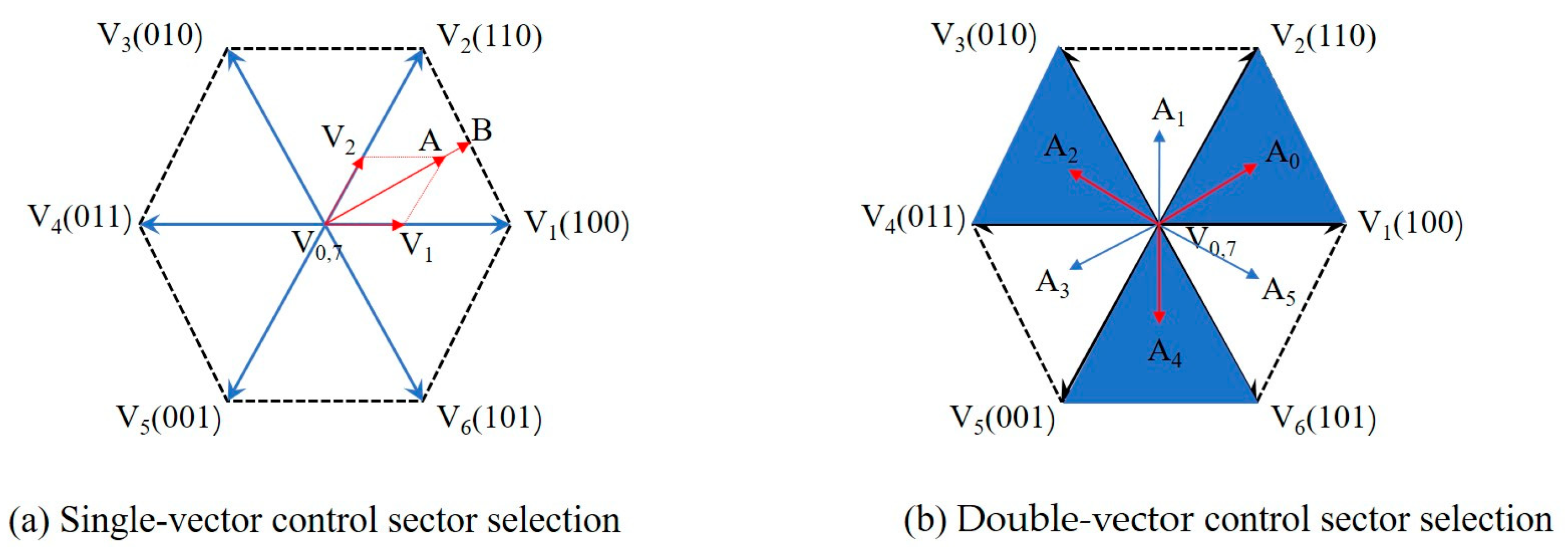[20,21] improved the event-triggered predictive control architecture for power converters by incorporating adaptive dynamic programming techniques and an event-triggering mechanism influenced by system uncertainties. Building on previous research, where control algorithms are often complex, this paper presents a double-vector control strategy that modifies the voltage selection method in the existing finite-control-set model predictive control (MPC). This strategy involves selecting voltage vectors twice within a single control cycle, with the second selection allowing for any direction. Consequently, this approach enhances the accuracy of voltage vector selection. Moreover, the method is straightforward and effectively reduces current fluctuations, thereby providing a solid foundation for precise motor control.

Building on the analysis and considerations outlined above, we first propose a flat rectangular slot structure suitable for permanent magnet synchronous linear motors. Second, we modify the finite-set model predictive control (FSMPC) by incorporating double-vector control, thereby altering the voltage selection process in traditional FSMPC. Finally, we implement this modified control strategy in an active suspension system to regulate the car body’s elevation to the target height. This approach not only reduces energy consumption but also enhances the car body’s responsiveness and ability to maintain the target height. Our method offers novel insights for improving vehicle stability and energy efficiency.

The subsequent sections are organized as follows: Section 2 shows the design of the main structural parameters of the linear motor; Section 3 shows the design of the permanent magnet synchronous linear motor double-vector control strategy; Section 4 details the body height controller design; Section 5 is the simulation result analysis; and Section 6 offers the conclusion and discussion.

2. Design of Key Structural Parameters for Linear Motors

2.1. Design Linear Motor Structure

The model shown in Figure 1 is built in Ansys Maxwell software.

The motor structure is designed as shown in Figure 1. In this design, considering its application in vehicle suspension systems, a flat rectangular slot is utilized for ease of manufacturing and installation. The total length of the actuator is set at 353 mm, while the total length of the stator is set at 224 mm.

The main dimensional parameters of the motor are shown in

Table 1. Main dimensional parameters of the motor.

Parameter	Meaning	Numerical/mm	Parameter	Meaning	Numerical/mm
hm	Thickness of permanent magnet	7.4	bs	Tooth–slot width	4.6
g	Air gap thickness	1	b0	End slot width	1.6
h0	Tooth root thickness	3.3	bt	End tooth width	8.7
hc	Axial length of coil	9.5	bmz	Axial pole width	5.3
hs	Height of stator yoke	6.3	bmr	Radial pole width	2.4
Ls	Stator length	224	Lt	Actuator length	353

:

2.2. Verification of the Rationality in Motor Structure Design

In order to verify the rationality of the motor structural design, a simulation was conducted, resulting in the magnetic flux density cloud map shown in Figure 2.

As shown in Figure 2, the magnetic saturation density of the motor is B < 1.8 T, indicating that there is no magnetic saturation; therefore, the motor parameter design is reasonable.

2.3. Parametric Modeling of the Motor

Parametric modeling of the linear motor was conducted, with the excitation selected as a current source. The phase currents of the primary winding were set to 4 A, 8 A, 12 A, 16 A, and 20 A, the simulation results are shown in Figure 3.

From the simulation results, it can be observed that when the current is 4 A, the average electromagnetic thrust reaches 1500 N, and at 8 A, it reaches 3000 N. This achieves the goal of high thrust with low current. In addition, to obtain the electromagnetic thrust constant required for double-vector control simulation, the curves in the figure were fitted, resulting in an electromagnetic thrust constant of kt = 0.14 N/A.

3. Design of Permanent Magnet Synchronous Linear Motor Double-Vector Control Strategy

3.1. Design of Double-Vector Control for PMSLM

The dual-vector model predictive current control operates on a two-stage optimization principle: after selecting the primary optimal voltage vector V_opt1 through vector control algorithms, a secondary optimization determines the second optimal voltage vector V_opt2. Unlike conventional approaches that restrict V_opt2 to zero vectors, this strategy enhances flexibility by dynamically adjusting the amplitude range (maximum/minimum) and spatial orientation of V_opt2 The cooperative action of dual vectors aims to minimize the tracking error between the actual and reference values of the d-axis current and q-axis current through composite modulation of V_opt1 and V_opt2 within one sampling period.

In the selection of V_opt2, the optimal voltage vector V_opt1 and seven voltage vectors are combined, respectively, and the action time of two voltage vectors in each combination is pre-allocated, and then the action time of two voltage vectors is taken into account when the mathematical model is used to predict the current. In this case, the Q-axis voltage $u_q{|}_{sw}$ and D-axis voltage $u_d{|}_{sw}$ (sw = 0:6) of the different voltage vectors are as follows:

$$u_q{|}_{sw}={\displaystyle \frac{t_{opt1}}{T_s}}{u}_q{|}_{opt1}+{\displaystyle \frac{T_s-t_{opt1}}{T_s}}{u}_q{|}_j$$

(1)

$$u_d{|}_{sw}={\displaystyle \frac{t_{opt1}}{T_s}}{u}_d{|}_{opt1}+{\displaystyle \frac{T_s-t_{opt1}}{T_s}}{u}_d{|}_j$$

(2)

where $u_q{|}_{sw}$ is the Q-axis voltage, $u_d{|}_{sw}$ is the D-axis voltage; the subscript sw represents different voltage vectors (sw = 0:6); $t_{opt1}$ is the operating time of the optimal voltage vector V_opt1; $u_d{|}_{opt1}$,$u_q{|}_{opt1}$ are the stator voltage d and q voltage components corresponding to the optimal voltage vector V_opt1; $T_s$ is the sampling time; and $u_q{|}_j$, $u_d{|}_j$ is the quadrature axis voltage component corresponding to the j voltage vector V_j (j = 0, 1, …, 6). The voltage values of each voltage vector are shown in

Table 2. Voltage value of each voltage vector.

V (Sa, Sb, Sc)	Vopt1	Vopt2
V0 (0, 0, 0)	0	0
V1 (1, 0, 0)	2/3	0
V2 (1, 1, 0)	1/3	$\sqrt{3}/3$
V3 (0, 1, 0)	−1/3	$\sqrt{3}/3$
V4 (0, 1, 1)	−2/3	0
V5 (0, 0, 1)	−1/3	$-\sqrt{3}/3$
V6 (1, 0, 1)	1/3	$-\sqrt{3}/3$

.

3.2. Linear Motor Finite-Set Model Predictive Control

In a two-level inverter-driven AC motor control system, the inverter generates eight switching states corresponding to seven distinct voltage vectors—six active vectors and two zero vectors, as illustrated in Figure 4. Accounting for the inherent hysteresis characteristics of digital control systems and incorporating finite-control-set model predictive control principles, the compensated discrete mathematical model of the linear motor yields the predicted d-axis and q-axis current values at the (k + 1)th instant as follows:

$$i_d^{*}{|}_{sw}(k+1)=i_d^{*}(k)+{\displaystyle \frac{T_s}{L_s}}\left[u_d{|}_{sw}-R_s{i}_d^{*}(k)+{\omega }_r(k)L_s{i}_d^{*}(k)\right]$$

(3)

$$i_q^{*}{|}_{sw}(k+1)=i_q^{*}(k)+{\displaystyle \frac{T_s}{L_s}}\left[u_q{|}_{sw}-R_s{i}_q^{*}(k)-{\omega }_r(k)L_s{i}_d^{*}(k)-{\omega }_r(k){\psi }_f\right]$$

(4)

where $i_d^{*}{|}_{sw}(k+1)$ is the D-axis current at time k + 1; $i_q^{*}{|}_{sw}(k+1)$ is the Q-axis current at time k + 1; the subscript sw represents different voltage vectors (sw = 0:6); $i_q^{*}(k)$ and $i_d^{*}(k)$ are the q and d axis currents of hysteresis compensation; $T_s$ is the sampling time; $L_s$ is the stator inductance; $R_s$ is the stator resistance; ${\omega }_r(k)$ is the rotor angular velocity at time k; and ${\psi }_f$ is the permanent magnet flux linkage. Equations (3) and (4) can be used to obtain the predicted values of the seven voltage vectors of the inverter in the next sampling period.

Seven current prediction values can be obtained by combining seven groups of voltage vectors and their operating times obtained by double-vector control, which are input into the following cost function:

$$\mathrm{g}=\left[i_d^{*}-i_d\left(k+1\right)\right]+\left[i_q^{*}-i_q\left(k+1\right)\right]$$

(5)

where $i_d^{*}$ is the given value of the D-axis component of the stator current; $i_q^{*}$ is the given value of the Q-axis component of the stator current, and $i_d(k+1)$ and $i_q(k+1)$ are the predicted values of the d and q axis currents at the next sampling time, respectively.

Therefore, this is equivalent to considering the effect of the action time on the selection of voltage vector in the value function, so that not only the voltage vector but also the action time can be optimized. On the one hand, the model predictive control (MPC) strategy can easily carry out multi-objective control. On the other hand, by pre-assigning the action time of the voltage vector, the value function selects the optimal combination of the voltage vector and the action time, which can ensure that the voltage vector of the final action is still the optimal, so the selection of the voltage vector is more accurate. The control specification/specified performance is outlined in

Table 3. Control specifications and imposed performances.

Category	Performance/Condition	Target/Constraint
Position tracking accuracy	Maximum steady-state error	≤10 μm
Dynamic response	Step response settling time	<0.15 s
Operating temperature	Ambient temperature range	−20∼60 °C

.

4. Body Height Controller Design

In order to illustrate the above elevating control, the model of a one-quarter vehicle damping adjustable vibration system is first established. According to Newton’s law of acceleration, the following differential equation is obtained:

$$\left\{\begin{array}{l}{m}_1{\ddot{z}}_1=k_2(z_2-z_1)+c({\dot{z}}_2-{\dot{z}}_1)-k_1(z_1-q)-{F_d}^{\prime }\\ m_2{\ddot{z}}_2=-k_2(z_2-z_1)-c({\dot{z}}_2-{\dot{z}}_1)+{F_d}^{\prime }\end{array}\right.$$

(6)

where $m_1$ is the unsprung mass, $m_2$ is the sprung mass, $z_1$ is the unsprung mass displacement, $z_2$ is the sprung mass displacement, ${\dot{z}}_1$ is the unsprung mass velocity, ${\dot{z}}_2$ is the sprung mass velocity, ${\ddot{z}}_1$ is the unsprung mass body acceleration, ${\ddot{z}}_2$ is the sprung mass body acceleration, $k_1$ is tire stiffness, $k_2$ is spring stiffness, $c$ is the damping coefficient, and ${F_d}^{\prime }$ is the control force that generates the lifting of the car body. In order to facilitate calculation and modeling, the controlling force direction is stipulated to be consistent with the lifting direction of the vehicle body. The mathematical model of filtering white noise is as follows: $\stackrel{·}{q}=-\alpha \nu q+\omega (t)$, where $\alpha$ is the empirical value obtained from experiments on different pavements, $\alpha$ = 0.1303 for Class B pavements and $\alpha$ = 0.12 for Class C pavements, and $\omega (t)$ is white noise.

The overall structure of the height control system is designed using a hierarchical approach, with the principle block diagram shown in Figure 5. When the vehicle encounters rugged or special terrain that requires adjustment of body posture, the body controller detects the target height.

First Level: Based on the road excitation signal q collected in real time and the thrust state of the linear motor, the vehicle dynamics model dynamically determines the actual height z₂. Through the proportional integral (PI) controller, the error adjustment is made between the calculated height z₂ of the model and the set target height z₂* (including the tuning of proportional and integral parameters), and the optimal Q-axis current reference value i_q* is generated. This provides the current leading component for double-vector control.

Second Level: By the PI controller, the D-axis current is stabilized at 0 A to achieve magnetic field orientation, and the Q-axis current is input into the cost function as the main control to optimize current control and output three-phase voltage. After that, the three-phase voltage is input into the inverter, and the pulse width modulation current in the A-B-C coordinate system is output. After the conversion between the d-q coordinate system of the current (direct axis and alternate axis) and the a-b-c coordinate system (phase current), the input is entered into the prediction model. Based on the current prediction model, the predicted current value of the next control period is obtained by performing a double-voltage-vector transformation. Finally, the deviation between the predicted current and the reference instruction is re-injected into the value function to realize dynamic rolling optimization and ensure the optimality of the switching signal.

Third Level: The high-precision inverter currents drive the permanent magnet synchronous linear motor (PMSLM) to generate adjustable electromagnetic thrust, which is converted into body displacement through the vehicle dynamic model. Force–displacement closed-loop control enables autonomous height adaptation under complex road conditions.

5. Simulation Result Analysis

To validate that the proposed double-vector control strategy has a significant effect on the elevation of the vehicle body, reduces fluctuations, and improves response speed, simulations were conducted using Matlab/Simulink. The target vehicle height was set to 0.1 m, and the simulation time was set to 30 s.

The parameters of the vehicle model are as follows in

Table 4. Vehicle parameter model.

Parameter	Meaning	Unit	Data
$m_1$	Unsprung mass	kg	40
$m_2$	Sprung mass	kg	357.25
$k_1$	Tire stiffness	N·m−1	2,300,000
$k_2$	Spring stiffness	N·m−1	34,000
$c$	Damping coefficient	N·s·m−1	2500

.

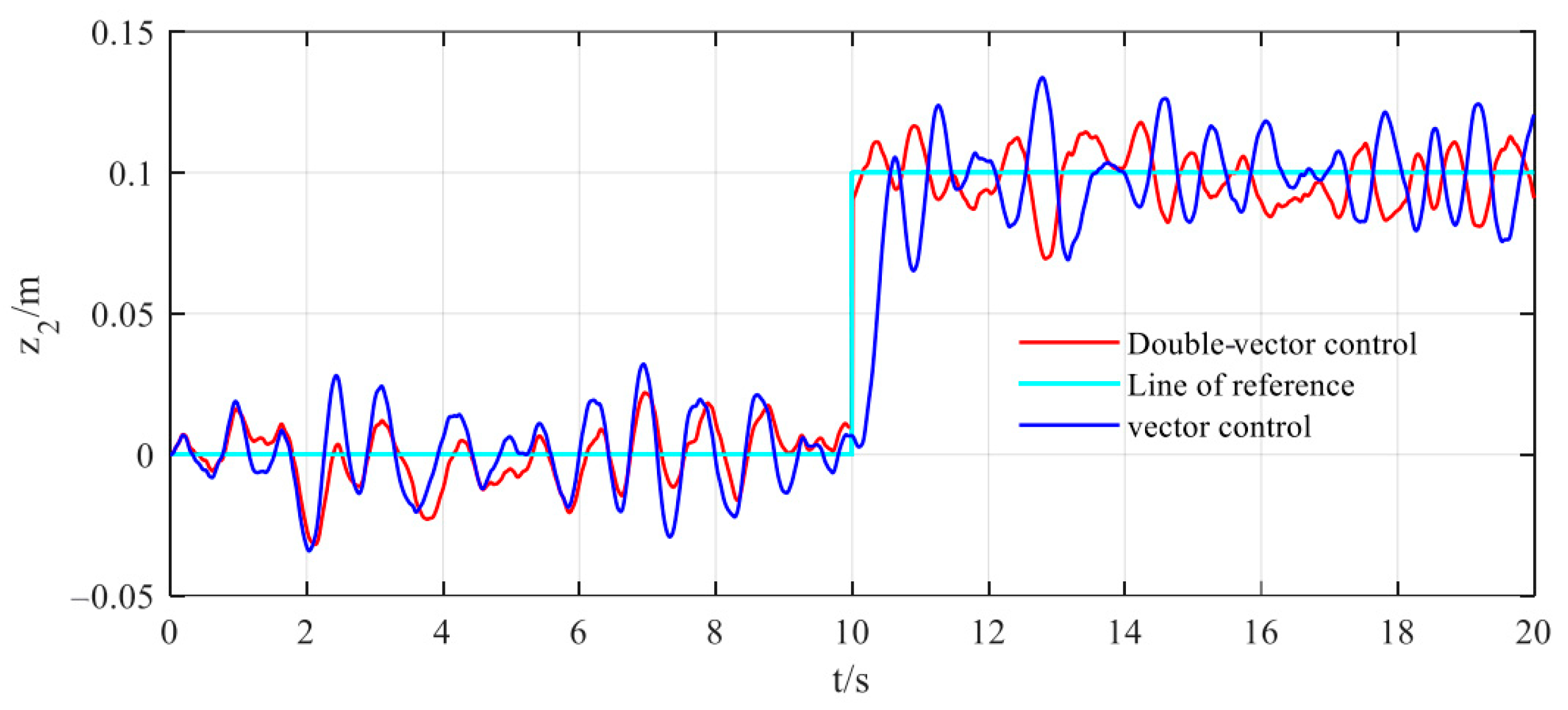
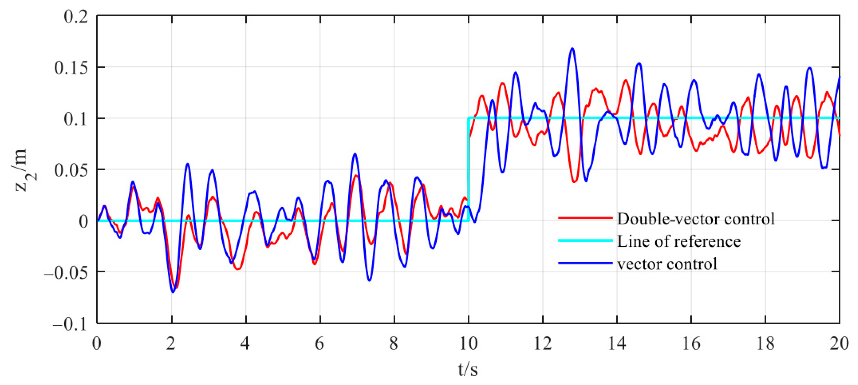
Simulation Condition 1: Control of the vehicle’s ascending motion. The target height of the vehicle is set at 0.1 m, with a speed of 20 m/s. The input excitation is set to Class B road conditions, and the simulation time is set for 20 s. At the 10 s mark, ascending control is implemented to drive the vehicle upward, and it ends at the 20 s mark. The simulation results are shown in Figure 6.

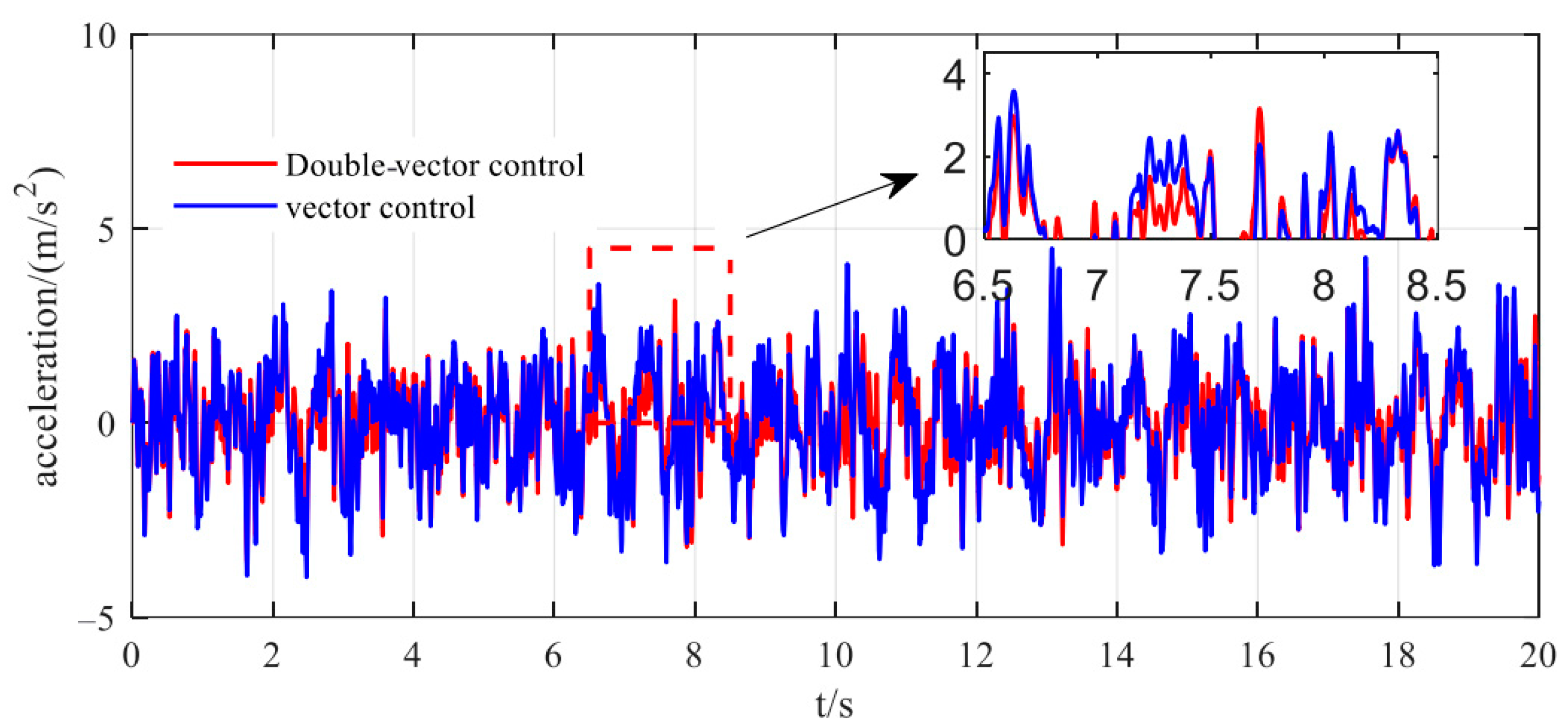
It can be seen from Figure 6’s sprung mass displacement that, within the first 10 s, the vehicle height fluctuates around the equilibrium position. At the 10 s mark, when adjusting the vehicle height, firstly, the fluctuation range of the vector control is approximately 0.065 m to 0.134 m, while the fluctuation range of the double-vector control is between 0.069 m and 0.118 m; the fluctuation amplitude has been reduced by about 70%. Secondly, the double-vector control reaches the target height within 0.15 s, whereas the vector control takes 0.56 s to reach the target height; the response speed has increased by about 23%. This indicates that the double-vector control has a significant effect on the smoothness of vehicle control. 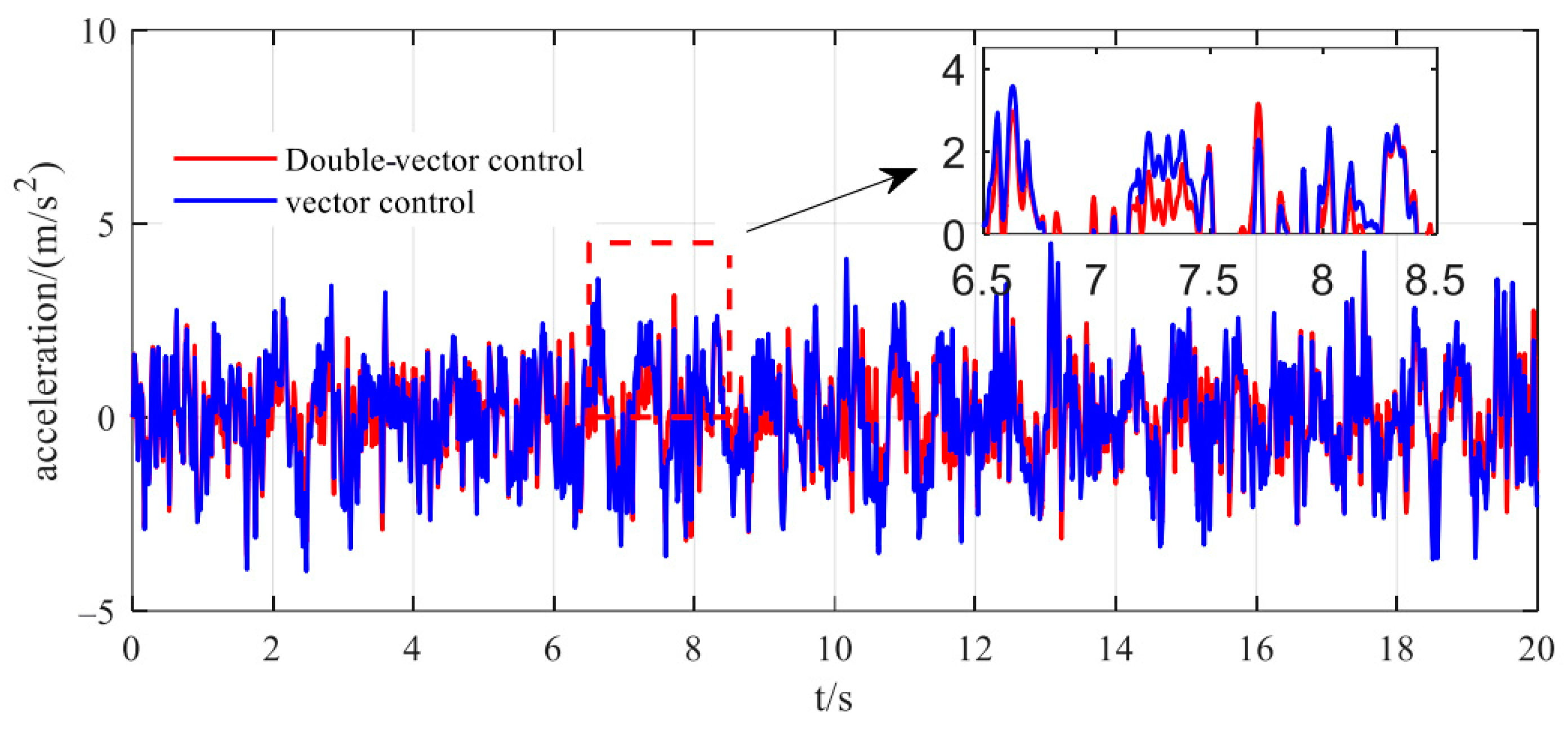Furthermore, as evidenced in Figure 7, the double-vector control strategy demonstrates superior performance over conventional vector control, reducing peak vertical body acceleration by 21.3% (from 3.8 m/s² to 3.2 m/s²) and improving vehicle ride comfort through a 17.6% decrease in Root Mean Square (RMS) values. 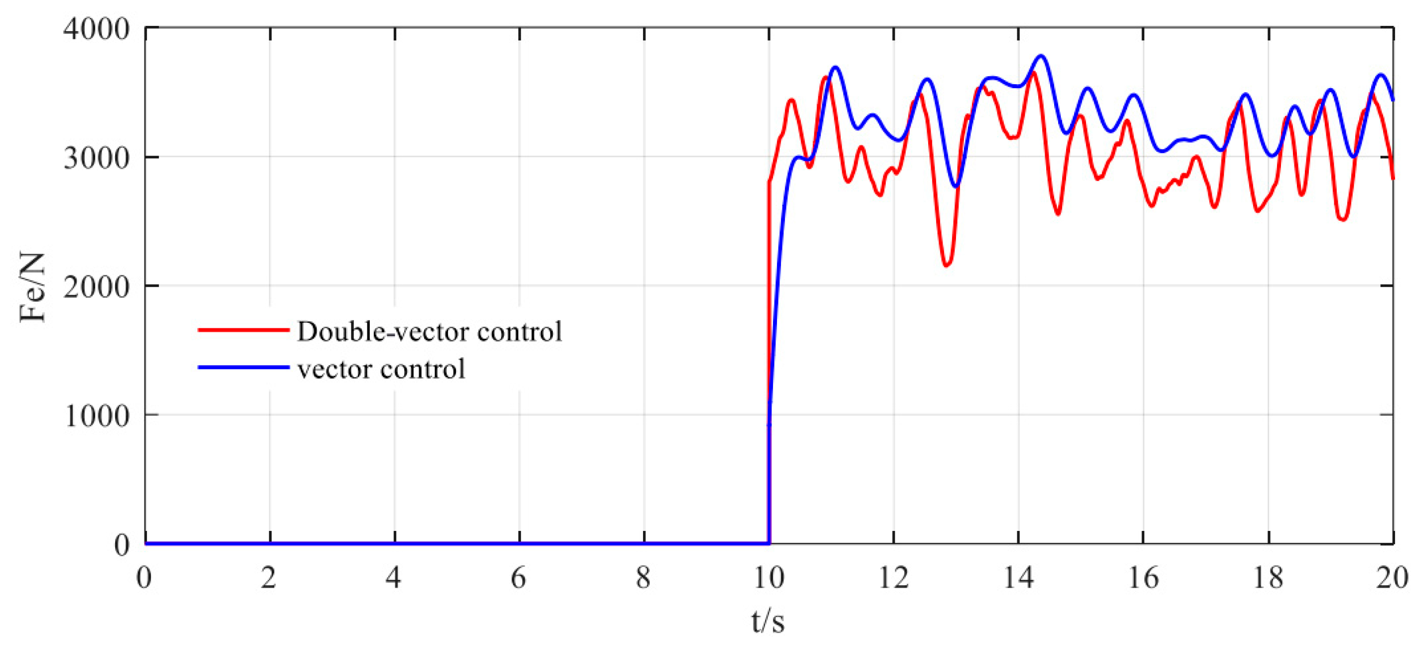The dynamic response characteristics in Figure 8 reveal that the double-vector system achieves a stabilized electromagnetic thrust output within 150 ms (mean: 3300 ± 35 N), representing a 5.7% reduction in required thrust compared to conventional vector control (mean: 3500 ± 42 N), confirming the strategy’s energy-saving efficacy. In order to facilitate understanding, an optimization performance comparison of vector control and double-vector control is made in

Table 5. Comparison of optimization performance of vector control and double-vector control (Ascent of 0.1 m, Class B Roadroad, 20 m/s).

Control Strategy	Sprung Mass Displacement Fluctuation	Maximum Body Acceleration Fluctuation	Electromagnetic Thrust
Vector control	0.065 m~0.134 m	3.8 m/s2	3500 ± 42 N
Double-vector control	0.069 m~0.118 m	3.5 m/s2	3300 ± 35 N

.

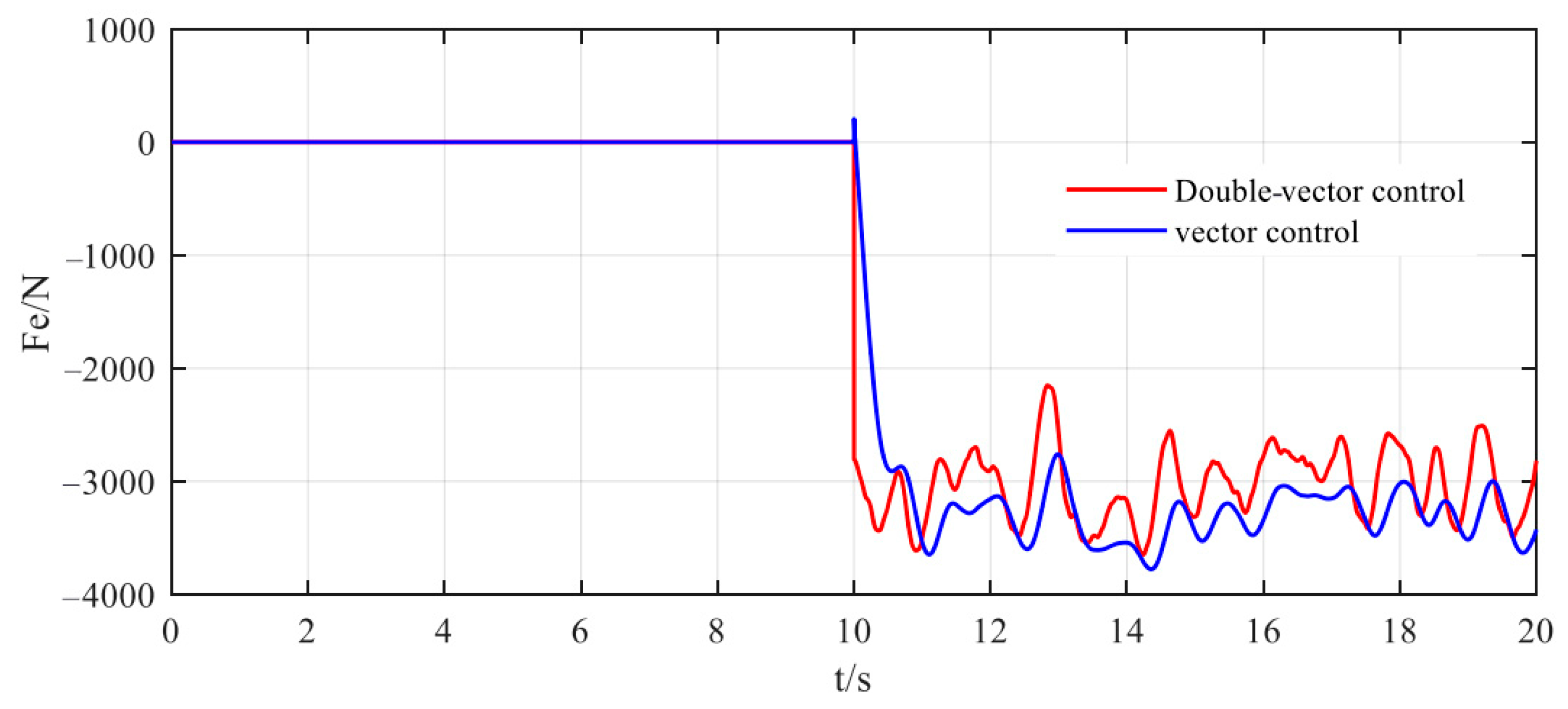
Simulation Condition 2: Control of the vehicle’s descending motion. The target height of the vehicle is set at −0.1 m, with the driving speed and road excitation conditions consistent with those of Simulation Condition 1. The simulation time is still set for 20 s. The difference is that descending control is implemented at the 10 s mark; it ends at the 20 s mark. The simulation results are shown in Figure 9, Figure 10 and Figure 11.

First, Figure 9 shows the displacement of the sprung mass. It can be observed that the effect of reducing the fluctuation amplitude is most significant; Figure 10 and Figure 11 illustrate the response curves of electromagnetic thrust and vehicle acceleration, which are generally consistent with Simulation Condition 1. Therefore, when we convert the vehicle’s ascending control into descending control, the double-vector control strategy maintains regulation performance in both electromagnetic thrust and vertical acceleration. In order to facilitate understanding, an optimization performance comparison of vector control and double-vector control is made in

Table 6. Comparison of optimization performance of vector control and double-vector control (Descent of 0.1 m, Class B Roadroad, 20 m/s).

Control Strategy	Sprung Mass Displacement Fluctuation	Maximum Body Acceleration Fluctuation	Electromagnetic Thrust
Vector control	0.063 m~0.137 m	3.7 m/s2	−3570 ± 42 N
Double-vector control	0.068 m~0.118 m	3.5 m/s2	−3320 ± 35 N

.

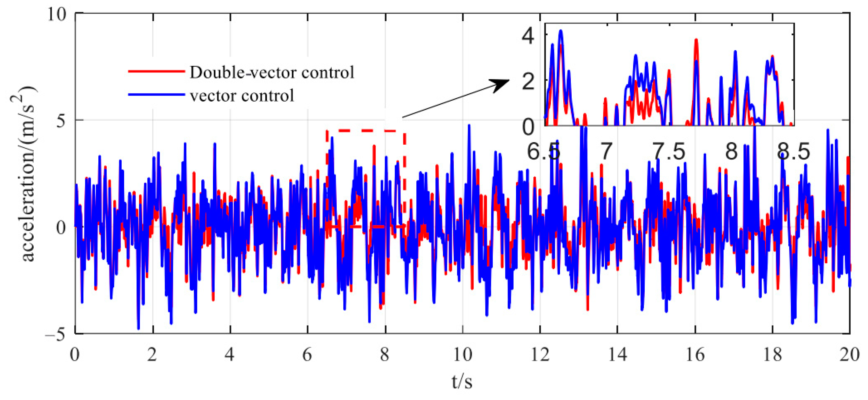
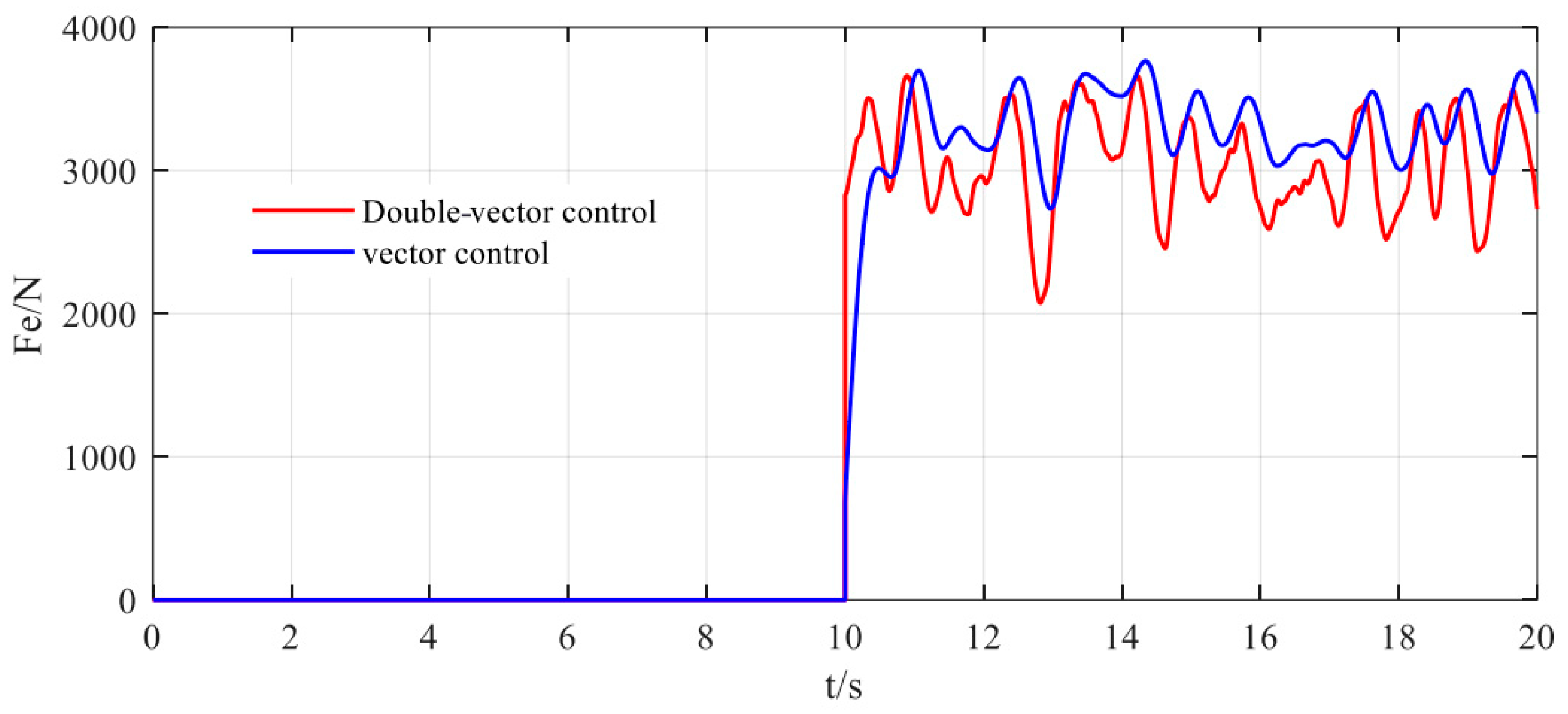
Simulation Condition 3: Control of the vehicle’s ascending motion. The target height of the vehicle, road excitation, simulation time, and lift/drop timing are all the same as in Simulation Condition 1. However, the driving speed is increased to 30 m/s. The simulation results are shown in Figure 12, Figure 13 and Figure 14.

Figure 12 shows the displacement of the sprung mass; it can be observed that during the vehicle’s ascent, the fluctuation in vector control ranges from approximately 0.063 m to 0.137 m, while the fluctuation in double-vector control ranges from 0.067 m to 0.118 m, and so the fluctuation amplitude has been reduced by about 70%. Additionally, double-vector control reaches the target height within 0.15 s, whereas vector control takes 0.56 s to reach the target height, leading to an improvement in response speed of approximately 23%.

Combining this with Simulation Condition 1, it can be concluded that this control algorithm maintains a good fluctuation reduction capability and response speed even at different vehicle speeds. Furthermore, as the speed increases, the fluctuations in vector control also increase, resulting in larger amplitude variations, while double-vector control exhibits minimal changes. From Figure 13 and Figure 14, the response curves for vehicle acceleration and electromagnetic thrust remain consistent with those in Simulation Condition 1. Therefore, even when the vehicle speed is increased, the desired vehicle height can still be achieved. In order to facilitate understanding, an optimization performance comparison of vector control and double-vector control is made in

Table 7. Comparison of optimization performance of vector control and double-vector control (Ascent of 0.1 m, Class B Roadroad, 30 m/s).

Control Strategy	Sprung Mass Displacement Fluctuation	Maximum Body Acceleration Fluctuation	Electromagnetic Thrust
Vector control	0.063 m to 0.137 m	4.2 m/s2	3720 ± 35 N
Double-vector control	0.067 m to 0.118 m	3.9 m/s2	3470 ± 42 N

.

Simulation Condition 4: Control of the vehicle’s ascending motion. The target height of the vehicle, simulation time, and lift/drop actions are all the same as in Simulation Condition 1, while the road excitation is changed to Class C. The simulation results are shown in Figure 15, Figure 16 and Figure 17.

From Figure 15, it can be concluded that during the vehicle’s ascent, the fluctuation in vector control ranges from approximately 0.038 m to 0.168 m, while the fluctuation in double-vector control ranges from 0.039 m to 0.137 m, resulting in a reduction of about 75% in fluctuation amplitude. Therefore, as the vehicle speed increases, the effectiveness of double-vector control in suppressing the displacement of sprung mass becomes increasingly evident. Additionally, double-vector control reaches the target height within 0.37 s, whereas vector control takes 0.92 s to achieve the same height, yielding an improvement in response speed of approximately 23%.

As can be seen from Figure 16 and Figure 17, the vehicle acceleration and the amplitude of the electromagnetic thrust response curves are still somewhat reduced. Therefore, even if the level of the road increases and the road becomes more rugged, the double-vector control can still achieve a better control effect. In order to facilitate understanding, an optimization performance comparison of vector control and double-vector control is made in

Table 8. Comparison of optimization performance of vector control and double-vector control (Ascent of 0.1 m, Class C Roadroad, 20 m/s).

Control Strategy	Sprung Mass Displacement Fluctuation	Maximum Body Acceleration Fluctuation	Electromagnetic Thrust
Vector control	0.038 m to 0.168 m	7.5 m/s2	4005 ± 35 N
Double-vector control	0.039 m to 0.137 m	7.1 m/s2	3805 ± 42 N

.

Combined with Simulation Conditions 1, 2, and 3, it can be seen that under different road excitation conditions and vehicle speeds, the control algorithm still has a good fluctuation reduction ability and response speed.

6. Conclusions and Discussion

A new control strategy for permanent magnet synchronous linear motor is proposed. The structural components of the motor are designed as a flat rectangular slot structure. For the motor control part, finite-set model predictive control (MPC) is used and corrected by double-vector control. On this basis, a multi-layer layered vehicle height controller is designed to optimize vehicle performance under complex road conditions. The simulation results show that the control strategy can effectively reduce the vibration amplitude of the vehicle, improve the response speed, reduce the thrust required to reach the target height, and achieve an energy saving effect. These findings have important contributions to future vehicle design and optimization, especially in terms of improving vehicle stability at different speeds and road conditions, as well as providing a theoretical basis for energy saving.

As shown in Figure 6, Figure 7, Figure 8, Figure 9, Figure 10, Figure 11, Figure 12, Figure 13, Figure 14, Figure 15, Figure 16 and Figure 17, the dual-vector control strategy significantly reduces sprung mass displacement fluctuations and improves dynamic response compared to conventional methods. This enhancement minimizes vertical vibration transmission, enhancing ride comfort on uneven road surfaces. Furthermore, effective suppression of peak body acceleration helps prevent unintended activations of electronic stability control (ESC) during emergency maneuvers, thereby improving handling safety. However, the dual-vector approach requires dual-voltage-vector optimizations per control cycle, resulting in substantially higher computational complexity than single-vector strategies. To achieve real-time control in high-dynamic scenarios, high-performance processors or dedicated hardware acceleration is necessary, imposing greater demands on onboard computational resources.

References

1. Yu, L.; Chang, S.; He, J.; Sun, H.; Huang, J.; Tian, H. Electromagnetic Design and Analysis of Permanent Magnet Linear Synchronous Motor. Energies 2022, 15, 5441. [Google Scholar] [CrossRef]
2. Mao, Y.; Sun, Z.; Zhou, W.; Zhuang, Z.; Qian, H. Electromagnetic Design of Toroidal Permanent Magnet Linear Synchronous Motor. IEEE Access 2021, 9, 98005–98012. [Google Scholar] [CrossRef]
3. Heidary, M.; Naderi, P.; Shiri, A. Modeling and analysis of a multi-segmented linear permanent-magnet synchronous machine using a parametric magnetic equivalent circuit. Electr. Eng. 2022, 104, 705–715. [Google Scholar] [CrossRef]
4. Wang, X.; Chen, F.; Zhu, R.; Huang, X.; Sang, N.; Yang, G.; Zhang, C. A Review on Disturbance Analysis and Suppression for Permanent Magnet Linear Synchronous Motor. Actuators 2021, 10, 77. [Google Scholar] [CrossRef]
5. Hao, W.; Zhang, G.; Liu, W.; Liu, H.; Wang, Y. Methods for Reducing Cogging Force in Permanent Magnet Machines: A Review. Energies 2023, 16, 422. [Google Scholar] [CrossRef]
6. Li, J.; Huang, X.; Zhou, B.; Yu, H.; Huang, Q. Design principle of a 16-pole 18-slot two-sectional modular permanent magnet linear synchronous motor with optimisation of its end tooth. IET Electr. Power Appl. 2020, 14, 441–447. [Google Scholar] [CrossRef]
7. Lan, Z.; Chen, L.; Xiao, X.; Luo, Y.; Deng, M.; Zhu, S. Detent force suppression of permanent magnet linear synchronous motor based on a V-shaped tooth-slot structure. IET Electr. Power Appl. 2023, 17, 535–546. [Google Scholar] [CrossRef]
8. Fu, D.; Wu, K.; Zheng, P.; Yu, Q.; Wu, X. Force Modeling and Analysis of a Tube Flux-Switching Transverse-Flux Permanent Magnet Linear Motor. IEEE Trans. Ind. Appl. 2022, 58, 4575–4586. [Google Scholar] [CrossRef]
9. Seal, M.; Sengupta, M. Optimised design, analysis, fabrication and experiments on a tubular linear induction motor prototype. Sadhana 2022, 47, 183. [Google Scholar] [CrossRef]
10. Mahdy, A.; Shaheen, A.; El-Sehiemy, R.; Ginidi, A.; Al-Gahtani, S.F. Single- and Multi-Objective Optimization Frameworks of Shape Design of Tubular Linear Synchronous Motor. Energies 2023, 16, 2409. [Google Scholar] [CrossRef]
11. Xu, W.; Elmorshedy, M.F.; Liu, Y.; Islam, R.; Allam, S.M. Finite-Set Model Predictive Control Based Thrust Maximization of Linear Induction Motors Used in Linear Metros. IEEE Trans. Veh. Technol. 2019, 68, 5443–5458. [Google Scholar] [CrossRef]
12. Xu, W.; Elmorshedy, M.F.; Liu, Y.; Rodriguez, J.; Garcia, C. Maximum Thrust per Ampere of Linear Induction Machine Based on Finite-Set Model Predictive Direct Thrust Control. IEEE Trans. Power Electron. 2019, 35, 7366–7378. [Google Scholar] [CrossRef]
13. Li, T.; Sun, X.; Lei, G.; Guo, Y.; Yang, Z.; Zhu, J. Finite-Control-Set Model Predictive Control of Permanent Magnet Synchronous Motor Drive Systems—An Overview. IEEE/CAA J. Autom. Sin. 2022, 9, 2087–2105. [Google Scholar] [CrossRef]
14. Kozubik, M.; Vaclavek, P. Speed Control of PMSM with Finite Control Set Model Predictive Control Using General-purpose Computing on GPU. In Proceedings of the IECON 2020 the 46th Annual Conference of the IEEE Industrial Electronics Society, Singapore, 18–21 October 2020; pp. 379–383. [Google Scholar]
15. Yao, J.; Cai, C.; Wang, S.; Yang, R.; Jia, Y. Hybrid model predictive control on lifting and dropping vehicle body via asymmetric damping adjustment. Veh. Syst. Dyn. 2023, 61, 3225–3243. [Google Scholar] [CrossRef]
16. Liu, C.; Yao, J.; Jia, Y. Vehicle height control based on active suspension with permanent magnet synchronous linear motor. Proc. Inst. Mech. Eng. Part D J. Automob. Eng. 2022, 238, 1191–1200. [Google Scholar] [CrossRef]
17. He, G.; Zheng, S.; Dong, Y.; Li, G.; Zhang, W. Model Predictive Voltage Control of Uninterruptible Power Supply Based on Extended-State Observer. Energies 2022, 15, 5489. [Google Scholar] [CrossRef]
18. Li, Z.; An, J.; Zhang, Q.; Liu, H.; Sun, H. Design of PMSLM Position Controller Based on Model Predictive Control Algorithm. IEEE Access 2021, 9, 78835–78846. [Google Scholar] [CrossRef]
19. Yin, Z.; Li, W.; Liu, J.; Zhang, Y. Adaptive Sliding-Mode-Based Speed Control in Finite Control Set Model Predictive Torque Control for Induction Motors. IEEE Trans. Power Electron. 2021, 36, 8076–8087. [Google Scholar] [CrossRef]
20. Liu, X.; Qiu, L.; Wu, W.; Ma, J.; Fang, Y.; Peng, Z.; Wang, D.; Rodriguez, J. Event-Triggered ESO-Based Robust MPC for Power Converters. IEEE Trans. Ind. Electron. 2023, 70, 2144–2152. [Google Scholar] [CrossRef]
21. Liu, X.; Qiu, L.; Fang, Y.; Wang, K.; Li, Y.; Rodríguez, J. Event-Driven Based Reinforcement Learning Predictive Controller Design for Three-Phase NPC Converters Using Online Approximators. IEEE Trans. Power Electron. 2025, 40, 4914–4926. [Google Scholar] [CrossRef]
Figure 1. Design of the motor structure.
Electronics 14 01515 g001
Figure 2. Magnetic flux density distribution of the motor at 0.01 s.
Electronics 14 01515 g002
Figure 3. Electromagnetic thrust at different current amplitudes.
Electronics 14 01515 g003
Figure 4. Sector selection of different control strategies for two-level inverters. (a) shows the principle of sector selection in single-vector control. The voltage vector space is divided into six sectors, each associated with one of the six non-zero basic voltage vectors V1 to V6, along with two zero vectors V0 and V7. In this illustration, the reference voltage vector lies between vectors V1 and V2. In single-vector control, the switching vector closest to the reference vector—such as V1 or V2—is selected for application. This method is simple to implement but has limitations in terms of control accuracy and waveform quality. (b) presents the sector division strategy used in double-vector control. Each of the six sectors is further divided to enhance control precision. The reference voltage V1 to V6 vectors can be synthesized using a weighted combination of two adjacent active vectors and a zero vector. This approach allows more accurate tracking of the desired voltage vector, leading to reduced current ripple, lower harmonic distortion, and smoother force output.
Electronics 14 01515 g004
Figure 5. Control diagram for vehicle body height adjustment.
Electronics 14 01515 g005
Figure 6. Displacement of sprung mass during an ascent of 0.1 m (Class B road, 20 m/s).
Electronics 14 01515 g006
Figure 7. Body acceleration during an ascent of 0.1 m (Class B road, 20 m/s).
Electronics 14 01515 g007
Figure 8. Electromagnetic force during an ascent of 0.1 m (Class B road, 20 m/s).
Electronics 14 01515 g008
Figure 9. Displacement of sprung mass during a descent of 0.1 m (Class B road, 20 m/s).
Electronics 14 01515 g009
Figure 10. Body acceleration during a descent of 0.1 m (Class B road, 20 m/s).
Electronics 14 01515 g010
Figure 11. Electromagnetic force during a descent of 0.1 m (Class B road, 20 m/s).
Electronics 14 01515 g011
Figure 12. Displacement of sprung mass during an ascent of 0.1 m (Class B road, 30 m/s).
Electronics 14 01515 g012
Figure 13. Body acceleration during an ascent of 0.1 m (Class B road, 30 m/s).
Electronics 14 01515 g013
Figure 14. Electromagnetic force during an ascent of 0.1 m (Class B road, 30 m/s).
Electronics 14 01515 g014
Figure 15. Displacement of sprung mass during an ascent of 0.1 m (Class C road, 20 m/s).
Electronics 14 01515 g015
Figure 16. Body acceleration during an ascent of 0.1 m (Class C road, 20 m/s).
Electronics 14 01515 g016
Figure 17. Electromagnetic force during an ascent of 0.1 m (Class C road, 20 m/s).
Electronics 14 01515 g017