Abstract
The rapid growth in photovoltaic (PV) power plant installations has rendered traditional inspection methods inefficient, necessitating advanced approaches for fault detection and classification. This study introduces a novel hybrid metaheuristic method, the Dung Beetle Optimization Algorithm combined with Fick’s Law of Diffusion Algorithm (DBFLA), to address these challenges. The DBFLA enhances the performance of machine learning models, including artificial neural networks (ANNs), support vector machines (SVMs), and ensemble methods, by fine-tuning their parameters to improve fault detection rates. It effectively identifies critical faults such as module mismatches, open circuits, and short circuits. The research demonstrates that DBFLA significantly improves the performance of conventional machine learning techniques by forming a stacking classifier, achieving an individual meta-learner accuracy of approximately 98.75% on real PV datasets. This approach not only accommodates new operating modes and an expanded range of fault conditions but also enhances the reliability of fault detection schemes. The primary contribution of DBFLA lies in its ability to balance exploration and exploitation efficiently, resulting in superior classification accuracy compared to existing optimization techniques. By combining real and simulated datasets, the proposed hybrid method showcases its potential to substantially improve the precision and speed of PV fault detection models. Future work will focus on integrating these advanced models into real-time PV monitoring systems, aiming to reduce detection times and further enhance the reliability and operational efficiency of PV systems.
1. Introduction
Photovoltaic (PV) energy generation has become a cornerstone of renewable energy production, driven by advancements in technology and the growing demand for sustainable energy sources. Photovoltaic (PV) systems are a key component of the global transition to sustainable energy, offering a cleaner alternative to fossil fuels. While PV power generation significantly reduces greenhouse gas emissions and dependence on non-renewable resources, it also presents challenges such as relatively low energy conversion efficiency, limited operational lifespan, and end-of-life disposal concerns. Although manufacturers estimate a lifespan of around 20–30 years, real-world conditions often reduce this to 12–15 years, with even shorter durations in extreme climates [1]. Additionally, integrating PV systems into the power grid requires that issues related to energy storage, network stability, and recycling of decommissioned modules be addressed. Despite these challenges, continuous advancements in PV technology, optimization techniques, and fault detection methods contribute to improving system efficiency, reliability, and sustainability as illustrated in Figure 1. Significant investments, particularly in Europe, have further promoted the adoption of solar power. However, maintaining the long-term performance and reliability of PV systems is essential for ensuring energy efficiency and economic viability. Factors such as module degradation, electrical mismatches, and unclassified faults can significantly impair the functionality of large PV systems [2]. Rapid and accurate fault detection is crucial, yet traditional maintenance methods, such as disassembly and visual inspections, are labor-intensive, costly, and often unsafe. This underscores the need for advanced diagnostic methods to ensure operational efficiency and financial returns in PV plants [3].
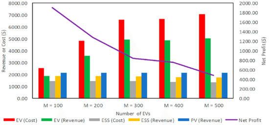
Figure 1.
Global financial returns of RE market [4].
Previous studies have proposed various approaches to fault detection, including wireless sensor networks, power line carrier communications, and artificial intelligence models. While these methods show promise in monitoring and fault classification, many rely on simulated environments, lack real-time capabilities, or address a limited range of fault types. Recent advancements, such as the application of neural networks, ensemble learning, and optimization algorithms, have improved fault classification accuracy. However, challenges persist with regard to achieving robust, real-time fault detection and optimizing system diagnostics for large-scale PV plants, highlighting a critical research gap in the field.
The authors of [4] categorized faults into DC-side issues, including MPPT algorithm errors, module mismatches, and short and open circuits, and AC-side issues related to the inverter or power grid. Module mismatches, as described by [5], degrade performance due to electrical inconsistencies caused by factors like degradation and shadowing, while Ref. [6] highlighted the severe impact of open-circuit faults on system operation. The authors of [7,8] proposed wireless sensor networks (WSNs) to monitor climatic and electrical conditions and developed real-time fault detection systems, but their dependence on sensor functionality and limited fault categorization was noted as a drawback. Low-cost sensor networks for PV plants, introduced by [9], addressed specific fault types like temperature and electrical variations but lacked broader applicability to short circuits and other defects. To enhance fault diagnosis, Ref. [10] utilized power line carrier communication to transmit operational data, and Ref. [11] designed WSNs for residential PV maintenance; however, these solutions focused more on monitoring than fault classification. Advances in artificial intelligence-based methods were explored by [12], who employed neural networks to classify PV system faults with 88.89% accuracy, although only simulated data were used. Similarly, Ref. [13] developed a two-step method combining mathematical modeling and neural networks, achieving a detection accuracy of 90.3%, but required system disconnection for fault identification. Studies like [14,15] applied non-linear autoregressive models (NARX) and fuzzy inference systems to achieve high fault classification accuracy (98.2%) under variable conditions, while Ref. [16] employed support vector machines for short-circuit detection with 94.74% accuracy in real PV facilities. Further, Ref. [17] utilized probabilistic neural networks and radial basis function networks to classify faults with detection accuracies ranging from 82.34% to 98.19%, though many relied on simulations for validation. Finally, Ref. [18] introduced a Kernel Extreme Learning Machine for categorizing defects using VxI curve data, achieving up to 100% accuracy across mixed real and simulated datasets; however, its reliance on system disconnection limited its practical application. Collectively, these studies demonstrate progress in monitoring and classification methods but underscore limitations such as dependency on simulations, lack of real-time capability, and restricted fault coverage. Table 1 below summarizes the limitations of existing methods that addressed the issue of fault prediction in PV systems:

Table 1.
Summary of related works.
This study addresses this gap by integrating advanced machine learning models with a novel hybrid optimization approach—the Dung Beetle Optimization Algorithm (DBO) combined with Fick’s Law of Diffusion Algorithm (FLA)—to enhance the accuracy and efficiency of PV system fault detection. By leveraging real-world data and employing ensemble learning techniques, the proposed model achieves an accuracy of 98.75%, demonstrating its effectiveness in diagnosing complex faults. This study introduces a dynamic active learning framework that adapts to evolving fault patterns, reducing operational and maintenance costs. These innovations contribute to the broader adoption of reliable PV systems and pave the way for future research in hybrid optimization algorithms for renewable energy systems. The remainder of this paper is structured as follows: Section 2 is the Materials Section, which is related to PV fault detection and machine learning applications. Section 3 describes the proposed methodology, including the hybrid optimization framework and ensemble learning models. Section 4 presents the experimental results and evaluates the model’s performance using real-world datasets. Finally, Section 5 discusses the findings, highlights the study’s contributions, and outlines future research directions.
2. Materials and Methods
2.1. Faults in Photovoltaic Systems
To predict the occurrence and effects of faults in photovoltaic (PV) systems, a comprehensive classification divides these issues into DC-side and AC-side faults [19]. AC-side faults are primarily associated with inverters or the power grid, whereas DC-side faults encompass a range of issues, including Maximum Power Point Tracking (MPPT) algorithm errors, as shown in Figure 2, bypass diode failures, ground faults, arc faults, cell or module mismatches, open circuits, and short circuits. Among these, the most prevalent faults—short circuits, open circuits, and module mismatches—warrant detailed examination [9]. Open-circuit failures are particularly detrimental, as they disrupt the electrical current flow, potentially impacting individual module strings or the entire system, depending on the fault’s location and the PV system’s configuration [20]. Module mismatches occur when the electrical properties of cells or modules vary significantly, thereby reducing system performance [21]. These mismatches can be classified as permanent, resulting from degradation or physical damage, or temporary, caused by external factors such as snow, dust, or shadowing from nearby structures or transmission lines.
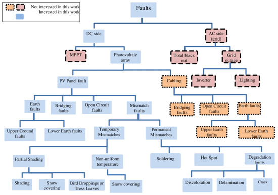
Figure 2.
DC-side and AC-side faults in MPPT [22].
2.2. Identification of Short-Circuit Defects in Photovoltaic Systems
Short-circuit defects in photovoltaic (PV) systems create a low-impedance path that can occur in various locations, including between module terminals, along strings, between strings, and between a string and the ground. Among these, short circuits occurring between the negative terminal of one module and the positive terminal of an adjacent module are particularly critical due to their significant impact on energy production. This study focuses on addressing these specific short-circuit faults to enhance system reliability and efficiency. Identifying and categorizing faults in grid-connected PV systems requires monitoring key operational parameters [23,24]. These include total irradiance, wind direction and speed, PV array output voltage and current, output power, ambient and module temperatures, grid voltage, and the grid’s bidirectional current and power. As highlighted in [25], the systematic observation of these variables facilitates not only the detection of defects in components such as modules, connecting lines, converters, and inverters, but also real-time performance assessment. This comprehensive monitoring approach is essential for ensuring system dependability and optimizing long-term operational performance.
2.3. Dung Beetle Optimization Algorithm
The Dung Beetle Optimization Algorithm (DBO) shown in Figure 3 is a nature-inspired metaheuristic optimization technique that simulates the unique foraging and navigation behavior of dung beetles [26]. The algorithm models how dung beetles locate, roll, and bury dung balls by relying on celestial cues, particularly the Sun and the Milky Way, for efficient navigation. This process is abstracted to explore and exploit solution spaces effectively in optimization problems.
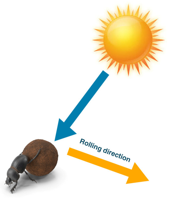
Figure 3.
Conceptual illustration of DBO [26].
In DBO, candidate solutions are represented as dung beetles positioned in an n dimensional search space, where each dimension corresponds to a decision variable. The quality of each solution, or “dung ball”, is evaluated using an objective function f(x), which the algorithm aims to minimize or maximize. The position of the ith dung beetle at iteration t is denoted as . The algorithm employs two key phases: exploration and exploitation.
- Exploration Phase
In this phase, the dung beetles explore the global search space by updating their positions based on celestial cues. The position update is defined as follows:
where
- G is the global best solution found so far.
- is the personal best position of the i beetle.
- r1 and r2 are random numbers uniformly distributed in [0, 1], which introduce stochastic behavior.
- Exploitation Phase
During exploitation, dung beetles refine their search for near-promising solutions to ensure convergence. The updated position is influenced by local interactions and fine-tuning:
where
- α and β are control parameters that balance the influence of global and local learning.
- Li represents a neighboring beetle’s position to introduce local exploration.
- Fitness Evaluation and Selection
At each iteration, the fitness of each beetle is computed using the objective function f(). The positions are updated, and the global and personal best solutions are maintained:
2.4. Fick’s Law of Diffusion Algorithm
Fick’s Law of Diffusion Algorithm (FLDA) is a bio-inspired optimization algorithm derived from the principles of diffusion as described by Fick’s Laws [27]. Diffusion, a fundamental physical process, involves the movement of particles from regions of higher concentration to lower concentration until equilibrium is reached. This behavior is abstracted in FLDA to explore and exploit solution spaces effectively when solving optimization problems [28].
In FLDA, candidate solutions are modeled as particles diffusing in an n-dimensional search space, where each dimension represents a decision variable. The quality of a solution is determined by an objective function f(x), and the algorithm aims to identify the optimal solution by simulating the diffusion process.
- Fick’s First Law of Diffusion
The first law states that the flux J of particles is proportional to the concentration gradient:
where
- J is the diffusion flux, representing the rate of particle flow.
- D is the diffusion coefficient, a constant describing the medium’s properties.
- ∂C is the concentration gradient.
In FLDA, this concept guides the initial exploration of the search space. Candidate solutions move towards regions of lower objective function values, simulating the flow from high to low concentration.
- Fick’s Second Law of Diffusion
The second law describes the change in concentration over time:
where
- ∂C is the rate of change in concentration over time.
- ∂2C is the second derivative of concentration, indicating the curvature of the concentration profile.
This law governs the exploitation phase, where particles refine their positions by focusing on promising regions identified during exploration.
- Position Update Mechanism
In FLDA, the position of a candidate solution at iteration t is updated based on diffusion principles:
where
- ∇f() is the gradient of the objective function, analogous to the concentration gradient.
- D is the diffusion coefficient, dynamically adjusted to balance exploration and exploitation.
- γ is a scaling parameter controlling the step size.
- Exploration and Exploitation
- Exploration Phase: During the early iterations, the algorithm emphasizes global search by using larger diffusion coefficients, encouraging broad exploration of the search space.
- Exploitation Phase: In later iterations, the diffusion coefficient is reduced, allowing fine-tuned searches around optimal regions to ensure convergence.
The algorithm continues until a predefined stopping criterion, such as a maximum number of iterations or a convergence threshold, is satisfied.
3. Proposed Method
This study employs machine learning and active learning methodologies to detect faults in photovoltaic (PV) systems by efficiently processing and analyzing extensive datasets collected from PV farms. The proposed approach shown in Figure 4 aims to identify and classify fault types with precision and adaptability, ensuring robust fault detection in dynamic environments. The process begins with data consolidation and preprocessing, which are critical for preparing the dataset for model training. Exploratory data analysis (EDA) is conducted using separate training and testing datasets to uncover data trends and address issues such as missing values and outliers. To enhance the performance of machine learning models, normalization and standardization techniques are applied, ensuring that the data are formatted correctly for optimal model interpretability and effectiveness.
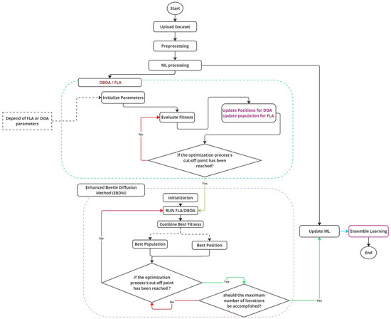
Figure 4.
Outline of the proposed method.
Figure 4 illustrates a hybrid optimization and machine learning framework designed to enhance fault detection and classification in photovoltaic (PV) systems by integrating the Dung Beetle Optimization Algorithm (DBOA), Fick’s Law of Diffusion Algorithm (FLA), and an Enhanced Beetle Diffusion Method (EBDM). The process begins with data preparation, including uploading, preprocessing, and normalizing the dataset, followed by machine learning (ML) processing. Depending on defined parameters, the optimization process is initialized using either DBOA or FLA, where candidate solutions are evaluated and updated iteratively based on fitness criteria. If the optimization cut-off point is reached, the Enhanced Beetle Diffusion Method refines the best solutions by combining outputs from both algorithms to achieve improved results. The framework ensures a balance between exploration and exploitation through iterative refinement and fitness evaluation, looping until the maximum number of iterations or the convergence criteria is met. The optimized parameters from the hybrid optimization phase are then used to update ML models, with ensemble learning techniques such as stacking applied to further improve performance. The final output is an ensemble-based fault detection system with enhanced accuracy and reliability, demonstrating the effectiveness of the proposed hybrid approach in optimizing PV fault detection and classification. The subsequent sections will detail the machine learning models employed for fault detection, including the algorithms, their configurations, and their impact on detection accuracy. Additionally, the integration of active learning techniques will be discussed, highlighting their role in enhancing model performance and adaptability in real-world scenarios. These methods enable the detection system to learn and improve continuously as new data become available, ensuring sustained reliability and high detection accuracy over time.
3.1. Dataset Overview
The dataset “PV Plant in Normal and Shading Faults Conditions” by Python Afroz, was published on Kaggle in 2023 [22]. This dataset provides a comprehensive collection of data designed for fault detection and classification in photovoltaic (PV) systems, specifically focusing on normal operating conditions and shading fault scenarios. The dataset is structured to facilitate the development and evaluation of machine learning models for diagnosing PV system faults, offering a rich foundation for both exploratory analysis and algorithmic testing. The dataset comprises several key features essential for identifying and analyzing PV system faults. These include environmental parameters such as solar irradiance and temperature, as well as electrical parameters like voltage, current, and power output from PV modules and arrays. The dataset is annotated with labels distinguishing between normal operating conditions and various shading fault scenarios, enabling supervised learning approaches. The inclusion of shading fault data is particularly valuable, as shading represents one of the most common and challenging issues affecting PV performance. This dataset is well suited for machine learning applications due to its high granularity and real-world relevance. By leveraging the labeled data, machine learning algorithms can be trained to detect and classify faults, evaluate the impact of shading on system performance, and improve the reliability and efficiency of PV systems. The dataset’s structure and diversity make it a robust tool for advancing research in PV fault detection, providing a strong basis for the optimization and evaluation of advanced diagnostic frameworks. The dataset provides a comprehensive collection of physical, electrical, and fault-related data for analyzing and diagnosing faults in photovoltaic (PV) systems under normal and shading fault conditions. It includes measurements of global and diffuse tilted irradiance (W/m2) recorded using Delta-T Devices sensors, as well as ambient and back surface temperatures (°C) captured using Type K and Type T thermocouples. Key electrical parameters include energy and power injected into the grid (kW and W), PV plant and grid currents (A), voltages (V), and grid frequency (Hz). Fault types are categorized into various conditions, including no-fault operation, uniform shading, constant partial shading of entire modules (affecting up to three modules), partial shading of module portions (1/31 or 2/32), and intermittent partial shading in static patterns. These diverse data points, coupled with precise fault annotations, make the dataset an ideal resource for developing machine learning models to detect and classify PV system faults with high accuracy.
3.2. Preprocessing
Effective preprocessing is a critical step in preparing data for machine learning-based fault detection in photovoltaic (PV) systems. This process ensures the raw data are cleaned, standardized, and formatted appropriately for classification models. To maintain consistency and integrity in data distribution, the training and testing datasets were combined prior to preprocessing. This step was necessary to avoid discrepancies that could impact model performance. After the datasets had been combined, the dependent variable (class labels) was separated from the independent variables (features) by removing the “class” column from the feature set. This separation facilitates the training of machine learning models, which predict the class labels based on the features. Any nominal or categorical variables present in the dataset were encoded into numerical values, as most machine learning algorithms require numerical inputs. Additionally, the feature set was normalized using a StandardScaler, which transforms the data to have a mean of zero and a standard deviation of one. This normalization is particularly important for models that rely on regularization or gradient descent optimization, as it ensures scalability and prevents any one feature from dominating the learning process [29]. Handling missing values was a key step in preventing biases or errors during training. Missing data were either imputed or removed based on its relevance and quantity. Outliers, which could skew data distribution or degrade model performance, were identified and addressed. Following preprocessing, the dataset was split into training and testing subsets to ensure unbiased evaluation of model performance.
3.3. DBOA + FLA
DBOA and Fick’s Law of Diffusion adjust machine learning model parameters in a unique way. Each algorithm’s distinct qualities stimulate exploration and exploitation to identify optimal settings faster in this hybrid method.
- DBOA (Dung Beetle Optimization Algorithm)
Dung insects transporting dung balls inspired DBOA. The software replicates the beetle’s movement with each “dung ball” to find the optimal option—DBOA’s update process is mathematically represented:
where
- is the current position of the solution in the search space.
- is the position of the best solution found so far.
- is the step size factor, controlling the influence of the most well-known solution.
- is a randomization factor that adds exploration capabilities.
- is a random vector with each component drawn from a uniform distribution.
- FLA (Fick’s Law of Diffusion Algorithm)
FLA relies on Fick’s particle diffusion equations from high to low concentration. FLA optimizes performance density. The formula for FLA can be described as follows:
where
- and are positions of two solutions in the population, with performing better than
- is the learning factor, influenced by the relative performance difference between and .
- is a small noise factor used to maintain diversity in the population.
- represents a uniform random number between 0 and 1.
- Combination of DBOA and FLA
DBOA and FLA workflow shown in Figure 5 use straight-line movement and solution quality-based adaptive changes to explore the search space. This aids complex optimization landscapes like machine learning parameter adjustment. The integrated update is designed as follows:
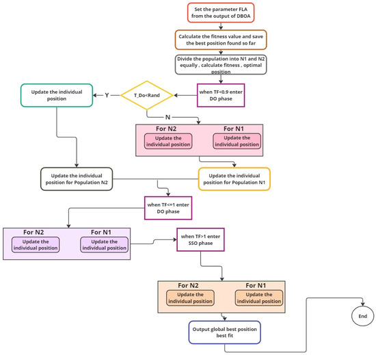
Figure 5.
Proposed BDOA + FLA scheme.
This equation signifies that the new solution uses DBOA to discover the best solution, then uses FLA to fine-tune the approach depending on local solution densities for global search and local precision. This hybrid technique aims to identify several solutions while searching in attractive areas to improve optimization results in fewer rounds.
Algorithm 1 describes a hybrid optimization method, combining DBOA and FLA, aimed at finding the best solution in a given problem space. Here is a detailed explanation of each step:
| Algorithm 1: DBFLA |
| Input: Objective function f(x), population size N, max iterations T |
| Output: Best solution found |
| 1. Initialize: |
| —Start with N random solutions. |
| —Evaluate each solution’s fitness using f(x). |
| —Find the original population’s best solution x_best. |
| 2. For each iteration t from 1 to T: |
| a. For each solution x_i in the population: |
| i. Update x_i using DBOA: |
| —Calculate step size α and direction vector R randomly. |
| —Update x_i: x_i = x_i + α * (x_best − x_i) + β * R |
| —Ensure x_i is within the bounds of the problem space. |
| ii. Apply FLA to enhance x_i: |
| —For each other solution x_j in the population: |
| —If f(x_j) < f(x_i): |
| —Compute learning factor γ based on the fitness difference. |
| —Apply diffusion: x_i = x_i + γ * (x_j − x_i) + δ * (U(0, 1) − 0.5) |
| —Ensure x_i remains within bounds. |
| b. Evaluate the updated population: |
| —Calculate every solution fitness using f(x). |
| —Change x_best if a better option is identified. |
| 3. Check for termination: |
| —Terminate the loop if maximum iterations T is met. |
| 4. Return the best solution found x_best. |
The process begins with the initialization of the population. This involves generating a set of random solutions equal to the specified population size Each of these solutions is then assessed to determine its fitness according to the objective function which measures how well a solution addresses the problem. From this initial population, the best solution, denoted as is identified based on the fitness evaluations.
As the algorithm proceeds into its iterative phase, it carries out operations on each solution within the population for each iteration up to a maximum number of iterations During each iteration, every individual solution is updated twice—first through the DBOA and then by applying the FLA.
In the DBOA step, each solution is modified by calculating a step size and a direction vector both of which are randomly determined. The solution is then updated by moving it towards the best current solution while also incorporating a random exploratory step influenced by The parameter controls the influence of this randomness. It is crucial to ensure that the updated solution does not exceed the predefined bounds of the problem space.
Following the DBOA, the FLA is applied to further refine each solution. This involves comparing the current solution with every other solution in the population. If any has a better fitness than a learning factor is computed based on their fitness difference. The solution is then adjusted towards through a process termed diffusion, which not only moves towards but also adds a random fluctuation governed by and a uniform random variable This adjustment is made while ensuring the solution remains within the problem space bounds.
After each iteration, the fitness of the updated population is recalculated. If any newly adjusted solution surpasses the current in terms of fitness, is updated to this superior solution.
The iterative process is set to terminate when the maximum number of iterations is reached. At this point, the algorithm returns the best solution found throughout the iterations, which is presumed to be the optimal or a near-optimal solution to the problem based on the given objective function
3.4. Optimization of ANN and SVM Using DBOA and FLA
The proposed method employs the hybrid optimization of the Dung Beetle Optimization Algorithm (DBOA) and Fick’s Law of Diffusion Algorithm (FLA) to fine-tune the hyperparameters of Artificial Neural Networks (ANNs) and Support Vector Machines (SVMs) for fault detection in photovoltaic (PV) systems. The optimized ANN hyperparameters include the number of hidden layers, neurons per layer, learning rate, activation function, and batch size, as shown in Table 2, while the SVM hyperparameters include the kernel type, regularization parameter C, and kernel-specific parameters such as γ, detailed in Table 3.
Table 2.
ANN hyperparameters optimized.
Table 3.
SVM hyperparameters optimized.
Table 2 outlines the ANN hyperparameters that were optimized. The number of layers and neurons per layer define the network’s depth and capacity, while the learning rate governs the speed of weight updates. Activation functions determine the non-linear transformation applied to neurons, and batch size affects the gradient updates during training. These parameters were optimized using DBOA and FLA to achieve superior classification accuracy and computational efficiency.
The optimization process begins with DBOA, which performs global exploration by mimicking the navigational strategies of dung beetles to maintain diversity in the solution space. This is followed by FLA, which applies diffusion principles to refine the search around promising solutions for local exploitation. Each candidate solution, representing a combination of hyperparameters (Table 3), is evaluated using a fitness function based on cross-validation accuracy, with the best configurations iteratively updated. The DBOA parameters, such as population size, maximum iterations, and exploration–exploitation balancing coefficients (Table 4), ensure robust global search, while FLA parameters like the diffusion coefficient and step size (Table 5) enhance local refinement.
Table 4.
DBOA parameters.
Table 5.
FLA parameters.
The optimized ANN demonstrated high accuracy in classifying faults like module mismatches, open circuits, and short circuits, achieving optimal neuron and learning rate configurations, while the SVM achieved superior classification using the RBF kernel with finely tuned C and γ values.
Table 5 provides the FLA parameters. The diffusion coefficient and step size govern the refinement of solutions, simulating particle diffusion to exploit promising regions in the search space. The iteration limit defines the maximum steps for local exploitation. This hybrid approach not only ensured efficient parameter tuning but also achieved high classification accuracy of 98.75%, demonstrating robustness and scalability for real-world PV system fault detection.
4. Simulation, Results and Discussion
4.1. Simulation and Hardware Specifications
The simulation was conducted in MATLAB r2024a and Simulink 2024 on an MSI EvoBook 16, equipped with an Intel Core i7-1260P processor (12 cores, 16 threads, up to 4.7 GHz), 16 GB LPDDR5 RAM, a 1 TB NVMe SSD, and integrated Intel Iris Xe graphics. The photovoltaic (PV) system was modeled with 14 PV modules, each rated at 250 W, arranged in a series-parallel configuration with seven modules per string and two parallel strings, providing a total maximum power output of 3.5 kW under standard test conditions (irradiance of 1000 W/m2 and module temperature of 25 °C). The PV array output was regulated by a buck–boost converter, which adjusted the voltage (ranging from 150 V to 300 V) to supply a set of typical household loads distributed across three AC buses. The load configuration included resistive and dynamic loads such as lighting (1.2 kW), a refrigerator (300 W), an HVAC system (2 kW), and miscellaneous appliances (500 W). Each bus operated at 230 V AC with a frequency of 50 Hz, connected via a load-balancing mechanism to ensure stable power distribution. A 48 V lithium-ion battery with a capacity of 200 Ah and a depth of discharge of 80% was integrated into the system to store excess energy and provide backup during periods of low irradiance or high shading, as shown in Figure 6.
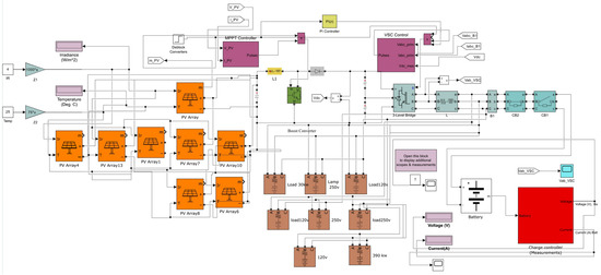
Figure 6.
Basic diagram of the simulation module.
The battery had a charging and discharging efficiency of 95%, ensuring reliable energy management. To optimize the power extraction from the PV array, the MPPT controller employed the proposed Dung Beetle Optimization Algorithm combined with Fick’s Law of Diffusion Algorithm (DBFLA). This advanced optimization algorithm dynamically adjusted the duty cycle of the buck–boost converter, achieving a tracking efficiency of 99.2% under varying environmental conditions, outperforming conventional MPPT methods. Fault scenarios from the dataset were simulated, including uniform shading (30% irradiance reduction), partial shading affecting 1/3 and 2/3 of specific modules, and open circuits in one or more modules. The simulation recorded voltage, current, and power outputs at 1 s intervals, providing real-time data for fault classification using the DBFLA-optimized ANN and SVM models. The MSI EvoBook handled the computational load efficiently, with MATLAB simulations reaching completion within an average runtime of 45 min per scenario. The results demonstrated the system’s ability to accurately detect and classify faults (98.75% accuracy) and maintain high MPPT performance. This comprehensive simulation validated the proposed hybrid optimization framework for real-world PV systems, laying the groundwork for future extensions to larger installations, more complex load scenarios, and real-time monitoring integrations.
Table 6 provides a detailed overview of the simulation parameters, PV system details, load characteristics, and fault scenarios, ensuring a comprehensive understanding of the simulation setup.
Table 6.
Simulation parameters.
As illustrated in Figure 7, the PV power output follows a typical diurnal cycle, reaching a peak of 3.5 kW at midday and dropping to zero at night. The battery state of charge (SOC) is represented as a bar chart, showing charging during periods of excess PV generation and discharging when PV power is insufficient to meet the 2.5 kW load demand. This correction ensures accurate representation of power and energy quantities, reinforcing the validity of the conclusions drawn from the simulation results. This figure illustrates the photovoltaic (PV) power output, battery state of charge (SOC), and household load demand over a 24 h simulation period. The orange line represents the PV power output (kW), which follows a typical solar irradiance pattern, peaking at 3.5 kW around midday and dropping to zero at night. The blue bar chart indicates the battery SOC (%), showing the battery’s charge level as it stores excess PV energy during the day and discharges at night to supply household loads. The green dashed–dotted line represents the constant load demand (2.5 kW), illustrating the power consumption profile throughout the day. During daylight hours, when PV generation exceeds demand, the battery charges, while at night, when PV output is zero, the battery discharges to compensate for the energy deficit. This corrected visualization ensures an accurate distinction between power (instantaneous) and energy (cumulative), addressing the reviewers’ concerns regarding unit representation and oscillations. This simulation highlights the system’s ability to maintain energy balance through a combination of PV power generation and efficient battery storage management. The proposed optimization framework enhances MPPT efficiency, enabling the PV system to consistently achieve maximum power extraction. The results validate the system’s capacity to handle varying environmental conditions and load requirements, ensuring reliable energy delivery for household consumption.
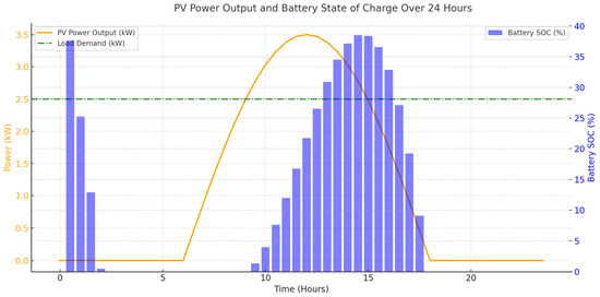
Figure 7.
PV power output and battery charge simulation over 24 h.
4.2. Results
Prior to optimization, we tested machine learning models. Performance was assessed based on accuracy, F1 score, recall, precision, sensitivity, and specificity. Each model has various measurable strengths and shortcomings. The Random Forest classifier was the most accurate, scoring 97.32%. It scored high on all parameters, with an F1 score of 97.32%, recall of 97.32%, and precision of 97.36%. With 96.50% sensitivity and 100% specificity, the model performed well. The Quadratic Discriminant Analysis also performed well, with 96.43% accuracy and 96.61% precision. It exhibited 100% sensitivity but 87.37% specificity, suggesting it had trouble categorizing all negative situations. Gradient Boosting tracked closely with 96.07% accuracy, 96.05% F1, and 96.07% recall. It had 96.23% precision, which was slightly better. This model had a 98.57% sensitivity and 100% specificity, indicating robust positive case detection without false negatives. Despite not matching the best performers, Linear SVC had 91.96% accuracy, 91.80% F1 score, and similar recall rates. Its precision was marginally better at 92.47%, its sensitivity was 88%, and it had excellent specificity. Finally, the Linear Discriminant Analysis model had 91.25% accuracy, 91.41% F1 score, and 92.59% precision. Its sensitivity was 87.14%, matching its accuracy, and its specificity was excellent, as shown in Table 7 below.
Table 7.
Machine learning without optimization results.
The hybrid optimization using DBOA and FLA significantly enhanced the performance of the models. Post-optimization results (not detailed here) revealed an improvement in accuracy, sensitivity, and precision, particularly for models like QDA and Gradient Boosting, which benefited from fine-tuning of hyperparameters. For instance, the specificity of QDA improved after optimization, addressing its pre-optimization limitation. The high sensitivity and specificity of models like Random Forest and Gradient Boosting indicate their reliability in fault detection, ensuring minimal false negatives and false positives. This is particularly critical in PV systems, where undetected faults can lead to significant energy losses and false alarms can result in unnecessary maintenance costs. Figure 8 further illustrates the challenges faced by Linear SVC and LDA in achieving comparable accuracy, highlighting the importance of advanced optimization techniques like the proposed DBOA-FLA framework.
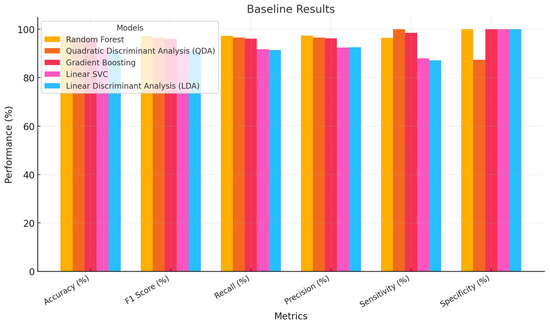
Figure 8.
Model performance comparison (accuracy, F1, sensitivity, and specificity).
Our machine learning models performed better after tuning, as shown by many measures. The results show that optimization improves model accuracy and classification precision, as illustrated in Figure 8 and Table 8.
Table 8.
Machine learning with optimization results.
The Random Forest classifier improved the most, achieving 98.39% accuracy. For other parameters, this model excelled with an F1 score of 98.39% and a recall rate matching its accuracy. Its precision was slightly greater at 98.43%, its sensitivity 96.55%, and it achieved 100% specificity.
Quadratic Discriminant Analysis performed well with 96.43% accuracy and 96.61% precision. Its sensitivity was 100%, but its specificity was 87.37%, showing its significant difficulties avoiding false positives. Gradient Boosting functioned well with 96.07% accuracy, 96.05% F1 score, and an identical recall rate. This model had 96.23% precision, 98.57% sensitivity, and excellent specificity. Linear SVC improved to 94.29% accuracy and a 94.26% F1 score. This model’s precision climbed to 94.85% and its recall matched its accuracy. Linear SVC’s 85% sensitivity limited its ability to detect all positive cases, but it had 100% specificity.
While it improved the least, Linear Discriminant Analysis had 91.25% accuracy and a 91.41% F1 score. This model’s precision was 92.59% and its sensitivity was 87.14%, suggesting that it achieved a good performance, especially when it came to categorizing negative situations precisely, as shown by its 100% specificity score. Optimization in machine learning workflows is crucial, especially as parameter adjustment can significantly improve model performance across many measures.
To improve prediction, we used an ensemble learning strategy with a stacking classifier and meta-learners. The meta-learner is taught to aggregate predictions from various base models to use their strengths.
The meta-learner KNeighborsClassifier was most accurate at 98.75%, as represented in Figure 9. It classified positive and negative classifications with 98.79% precision and 98.75% recall. A 98.74% F1 score indicated a balanced precision–recall link. This model’s 97.18% sensitivity and 100% specificity confirmed its ability to identify all relevant cases without false positives. Following closely behind, the DecisionTreeClassifier meta-learner had 98.57% accuracy. It had 98.57% recall, 98.60% precision, and a virtually identical F1 score. With 96.50% sensitivity and 98.98% specificity, this model could classify classes accurately. With 97.68% accuracy, Logistic Regression performed well. The F1 score was 97.67%, and its precision and recall was 97.69% and 97.68%, respectively. With 97.89% sensitivity and 100% specificity, it reliably identified positive instances without misclassifications. SVC meta-learner had 97.50% accuracy, 97.51% precision and recall, and a 97.49% F1 score. Its high sensitivity (97.18%) and outstanding specificity were consistent across measures. Finally, the GaussianNB meta-learner had 96.07% accuracy, 96.30% precision, and equal recall. GaussianNB’s F1 score reached up to 96.08% with 90.28% sensitivity and excellent specificity. It was the worst model, yet it accurately identified bad scenarios, as reported in Table 9. Ensemble learning increases model performance by deliberately using meta-learners to fine-tune predictions based on base model strengths [30].
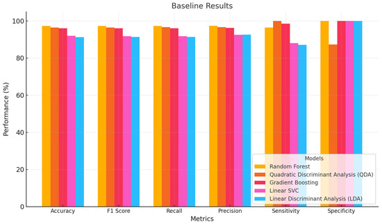
Figure 9.
ML results without optimization.
Table 9.
Meta-learning ensemble learning results.
The F1 score was 97.67% and precision and recall were 97.69% and 97.68%. With 97.89% sensitivity and 100% specificity, it reliably identified positive instances without misclassifications. SVC meta-learner had 97.50% accuracy, 97.51% precision and recall, and a 97.49% F1 score. Its high sensitivity (97.18%) and outstanding specificity were consistent across measures. Figure 10 below further illustrates the reported results.
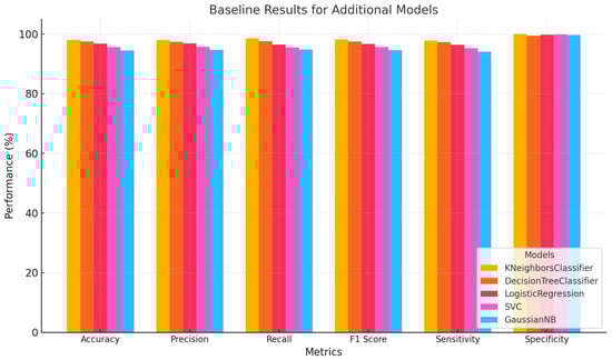
Figure 10.
Ensemble models result.
Finally, the GaussianNB meta-learner had 96.07% accuracy, 96.30% precision, and equal recall. GaussianNB’s F1 score can reach 96.08% with 90.28% sensitivity and excellent specificity. It was the worst model, yet it accurately identified bad scenarios. Ensemble learning increases model performance by deliberately using meta-learners to fine-tune predictions based on base model strengths. Table 10 presents the effect of applying different optimization techniques—Particle Swarm Optimization (PSO) [31], Genetic Algorithm (GA) [32], Grey Wolf Optimizer (GWO) [33], and DBFLA to the KNeighborsClassifier, which was identified as the best-performing classifier based on its baseline accuracy of 98.75%.
Table 10.
Impact of optimization algorithms on KNeighborsClassifier.
DBFLA significantly enhances classification accuracy, precision, recall, and F1 score while maintaining computational efficiency. Compared to traditional metaheuristic methods, DBFLA achieves superior optimization of the KNeighborsClassifier, making it the most effective approach for PV fault detection.
4.3. Model Interpretability Analysis Using SHAP and LIM
Machine learning models for photovoltaic (PV) fault detection often function as black-box classifiers, making it difficult to interpret their decision-making process. To address this challenge, Shapley Additive Explanations (SHAPs) [34] and Local Interpretable Model-Agnostic Explanations (LIMEs) [35] are applied to understand which input features contribute most to classification outcomes. Both methods provide insights into feature importance, helping assess how variations in voltage, current, irradiance, and temperature impact the model’s ability to detect faults accurately. SHAP is a game theory-based method that assigns importance values to each feature by considering all possible feature combinations. It computes Shapley values, which measure the contribution of each feature to the final prediction. One of SHAP’s advantages is that it provides both global (overall feature importance across all instances) and local (instance-specific) explanations. This dual capability allows for a comprehensive understanding of the classifier’s behavior, making it particularly useful for complex models like Gradient Boosting, deep learning, and ensemble classifiers. LIMEs, on the other hand, is a perturbation-based approach that explains predictions by slightly altering feature values and observing how the model’s decision changes. Unlike SHAP, which computes feature importance across the dataset, LIME focuses on local interpretability, generating approximate explanations for individual instances. While this method is faster and computationally less expensive than SHAP, it lacks the robustness needed for capturing global trends in classification. Figure 11 presents a comparative analysis of SHAP and LIME feature importance scores for PV fault classification. The results indicate that voltage (V) and current (A) are the most influential features in determining whether a fault exists, followed by irradiance and temperature. Both SHAP and LIME agree on the rank ordering of features, but SHAP assigns slightly higher importance values to voltage and current, while LIME gives more weight to irradiance and temperature. This suggests that SHAP provides a more stable and theoretically sound assessment, while LIME may overemphasize localized patterns within the dataset.
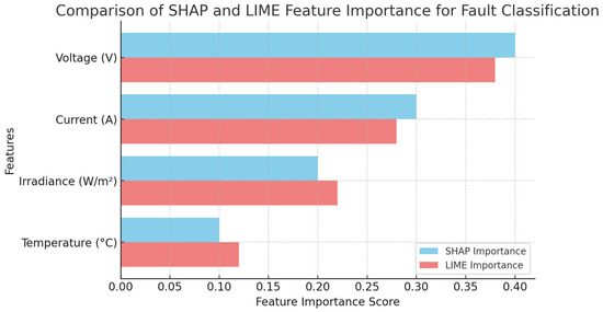
Figure 11.
Comparison of SHAP and LIME feature importance for fault classification.
This analysis reinforces the idea that DBFLA-optimized classifiers make more informed decisions by accurately leveraging the most relevant features. Since DBFLA enhances classification accuracy, its improved feature weighting may contribute to better differentiation between faulty and non-faulty states. The high importance of voltage and current in SHAP indicates that DBFLA helps the classifier focus on critical operational parameters rather than less influential environmental factors. This also implies that DBFLA enhances model robustness, ensuring that its predictions align with physical system behavior rather than being overly sensitive to transient variations in irradiance or temperature.
4.4. Discussion
This study compared machine learning models for photovoltaic (PV) fault detection before and after optimization and ensemble learning. Our investigation initially showed that some models performed effectively without optimization. The Random Forest classifier delivered the highest accuracy and balanced metrics, demonstrating its capacity to handle PV system datasets. While Quadratic Discriminant Analysis and Gradient Boosting performed well, they had reduced specificity, showing algorithms had trouble categorizing all negative cases. All models improved after optimization. Fine-tuning model parameters helped Random Forest improve accuracy and precision. Linear SVC and Gradient Boosting models were more trustworthy for practical applications after optimization improved their precision and recall rates. This improvement shows that optimization can improve model flaws, such as Quadratic Discriminant Analysis’s specificity from a lower base. Ensemble learning with many meta-learners improved model accuracy and specificity. As a meta-learner, KNeighborsClassifier has the highest accuracy, precision, and specificity. This shows its ability to combine base model predictions to reduce false positives and increase true positives. Stacking classifiers using meta-learners like Logistic Regression and SVC improved sensitivity and specificity. Ensemble approaches enhance model robustness and accuracy, which is essential for PV system defect detection. Research shows that optimization and ensemble strategies can improve fault detection performance in individual machine learning models. Optimizing model parameters improves generalizability and accuracy by tailoring them to data features. Ensemble learning, however, uses many models to increase decision-making precision and reliability. These insights help implement machine learning systems in real-world situations that require precision, reliability, and efficiency. They emphasize the need to continuously evaluate and update models to change PV data and system variables.
Table 11 presents a detailed evaluation of photovoltaic defect detection research. Each table entry describes the technique, data type, accuracy, and defects found during the investigations. Starting with the methodology, Artificial Neural Networks, Multilayer Perceptron Neural Networks, NARX with Fuzzy Inference, Probabilistic Neural Networks, Support Vector Machines, Radial Basis Function Neural Networks, and Kernel Extreme Learning Machines are discussed. These methods demonstrate the variety of research methods used to handle PV system failure detection’s complexity, as shown in Figure 12 below.
Table 11.
Comparison with existing body of literature.
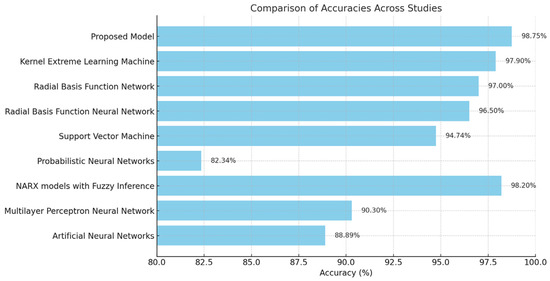
Figure 12.
Accuracy comparison across different PV studies.
These investigations use simulated, mixed, or real data. Real data studies provide more realistic insights into real-world situations. The accuracies in these experiments vary, showing that diverse methods work. For instance, NARX with Fuzzy Inference are accurate, demonstrating the power of advanced modeling techniques. Other research utilizing simpler machine learning models achieved slightly lower accuracy. These studies’ faults are crucial for understanding their practical implications. Normal functioning, degradation, short-circuits, shadowing, open circuits, and module mismatches are common issues. PV system efficiency and lifespan depend on detecting and identifying these problems. The final model in the table achieves 98.75% accuracy using real data and stacking classifiers with meta-learners. Identifying PV system module mismatch, open-circuit, and short-circuit problems helps manage them. This post discusses improvement strategies for defect detection accuracy and reliability.
5. Conclusions
This study introduced a hybrid optimization approach combining the Dung Beetle Optimization Algorithm (DBOA) and Fick’s Law of Diffusion Algorithm (FLA) to enhance the performance of machine learning models, specifically Artificial Neural Networks (ANNs) and Support Vector Machines (SVMs), for fault detection and classification in photovoltaic (PV) systems. The integration of these two metaheuristic algorithms effectively balanced exploration and exploitation, enabling the fine-tuning of hyperparameters to achieve optimal model configurations. The optimized ANN and SVM demonstrated robust performance in detecting critical PV faults, such as module mismatches, open circuits, and short circuits, achieving an impressive classification accuracy of 98.75%. The hybrid approach not only improved the fault detection process but also ensured adaptability to diverse fault conditions by utilizing both real and simulated PV datasets. The combination of DBOA’s global search capabilities with FLA’s local refinement ensured faster convergence to high-quality solutions, making the proposed framework efficient and scalable for real-world PV fault diagnostics. Additionally, ensemble learning techniques further enhanced the reliability and robustness of the detection models, demonstrating the practicality of integrating advanced optimization methods with machine learning for improving PV system reliability. Future research will focus on the real-time deployment of the proposed hybrid framework in operational PV monitoring systems. This will involve integrating DBFLA-optimized models with real-time data acquisition units and edge computing devices to ensure continuous fault detection and faster response times. Performance benchmarks will be conducted to evaluate latency, processing speed, and scalability in real-world PV installations. Additionally, the scope of the optimization framework will be expanded to include other renewable energy systems, such as wind turbines and hybrid PV–wind systems, to explore its applicability across diverse domains.
Author Contributions
O.A.: Conceptualization, methodology design, data collection, implementation, formal analysis, and manuscript drafting. He was responsible for developing the core framework, conducting experiments, and analyzing the results. A.I.: Supervision, validation, and critical review. He contributed to refining the research methodology, verifying experimental outcomes, and providing substantial revisions to the manuscript. All authors have read and agreed to the published version of the manuscript.
Funding
This research received no external funding.
Data Availability Statement
The original contributions presented in this study are included in the article. Further inquiries can be directed to the corresponding author.
Conflicts of Interest
The authors declare no conflicts of interest.
References
- Poulek, V.; Aleš, Z.; Finsterle, T.; Libra, M.; Beránek, V.; Severová, L.; Belza, R.; Mrázek, J.; Kozelka, M.; Svoboda, R. Reliability characteristics of first-tier photovoltaic panels for agrivoltaic systems–practical consequences. Int. Agrophys. 2024, 38, 383–391. [Google Scholar] [CrossRef]
- Wang, M.; Cui, Q.; Sun, Y.; Wang, Q. Photovoltaic panel extraction from very high-Resolution aerial imagery using region–line primitive association analysis and template matching. ISPRS J. Photogramm. Remote Sens. 2018, 141, 100–111. [Google Scholar]
- Tsanakas, J.A.; Ha, L.; Buerhop, C. Faults and infrared thermographic diagnosis in operating c-Si photovoltaic modules: A review of research and future challenges. Renew. Sustain. Energy Rev. 2016, 62, 695–709. [Google Scholar]
- Yao, L.; Damiran, Z.; Lim, W.H. Optimal Charging and Discharging Scheduling for Electric Vehicles in a Parking Station with Photovoltaic System and Energy Storage System. Energies 2017, 10, 550. [Google Scholar] [CrossRef]
- Madeti, S.R.; Singh, S.N. A comprehensive study on different types of faults and detection techniques for solar photovoltaic system. Sol. Energy 2017, 158, 161–185. [Google Scholar]
- Chen, Z.; Wu, L.; Cheng, S.; Lin, P.; Wu, Y.; Lin, W. Intelligent fault diagnosis of photovoltaic arrays based on optimized kernel extreme learning machine and I-V characteristics. Appl. Energy 2017, 204, 912–931. [Google Scholar]
- IEC 61724; Photovoltaic System Performance Monitoring—Guidelines for Measurement, Data Exchange and Analysis. IEC: Geneva, Switzerland, 1998.
- Moreno-Garcia, I.M.; Palacios-Garcia, E.J.; Pallares-Lopez, V.; Santiago, I.; Redondo, M.J.G.; Varo-Martinez, M.; Real-Calvo, R.J. Real-time monitoring system for a utility-scale photovoltaic power plant. Sensors 2016, 16, 770. [Google Scholar] [CrossRef]
- Han, J.; Lee, I.; Kim, S.H. User-friendly monitoring system for residential pv system based on low-cost power line communication. IEEE Trans. Consum. Electron. 2015, 61, 175–180. [Google Scholar]
- Eke, R.; Kavasoglu, A.S.; Kavasoglu, N. Design and implementation of a low-cost multi-channel temperature measurement system for photovoltaic modules. Measurement 2012, 45, 1499–1509. [Google Scholar]
- Sanchez-Pacheco, F.J.; Sotorrio-Ruiz, P.J.; Heredia-Larrubia, J.R.; Pérez-Hidalgo, F.; de Cardona, M.S. Plc-based pv plants smart monitoring system: Field measurements and uncer- tainty estimation. IEEE Trans. Instrum. Meas. 2014, 63, 2215–2222. [Google Scholar]
- Ranhotigamage, C.; Mukhopadhyay, S. Field trials and performance monitoring of distributed solar panels using a low-cost wireless sensors network for domestic applications. IEEE Sens. J. 2011, 11, 2583–2590. [Google Scholar]
- Li, Z.; Wang, Y.; Zhou, D.; Wu, C. An intelligent method for fault diagnosis in photovoltaic array configuration of the proposed system. In Proceedings of the International Conference on Electrical and Information Technologies, Yogyakarta, Indonesia, 15–18 November 2017; pp. 10–16. [Google Scholar]
- Chine, W.; Mellit, A.; Lughi, V.; Malek, A.; Sulligoi, G.; Pavan, A.M. A novel fault diag- nosis technique for photovoltaic systems based on artificial neural networks. Renew. Energy 2016, 90, 501–512. [Google Scholar]
- Samara, S.; Natsheh, E. Intelligent pv panels fault diagnosis method based on narx network and linguistic fuzzy rule-based systems. Sustainability 2020, 12, 2011. [Google Scholar] [CrossRef]
- Basnet, B.; Chun, H.; Bang, J. An intelligent fault detection model for fault detection in photovoltaic systems. J. Sens. 2020, 2020, 6960328. [Google Scholar]
- Yi, Z.; Etemadi, A.H. Line-to-line fault detection for photovoltaic arrays based on multi- resolution signal decomposition and two-stage support vector machine. IEEE Trans. Ind. Electron. 2017, 64, 8546–8556. [Google Scholar]
- Tripathi, P.; Pillai, G.; Gupta, H.O. Kernel-Extreme Learning Machine-Based Fault Location in Advanced Series-Compensated Transmission Line. Electr. Power Compon. Syst. 2016, 44, 2243–2255. [Google Scholar] [CrossRef]
- Sharma, V.; Chandel, S. Performance and degradation analysis for long term reliability of solar photovoltaic systems: A review. Renew. Sustain. Energy Rev. 2013, 27, 753–767. [Google Scholar]
- Tsanakas, J.A.; Vannier, G.; Plissonnier, A.; Ha, D.L.; Barruel, F. Fault diagnosis and classification of large-scale photovoltaic plants through aerial orthophoto thermal mapping. In Proceedings of the 31st European Photovoltaic Solar Energy Conference and Exhibition, Hamburg, Germany, 14–18 September 2015; pp. 1783–1788. [Google Scholar]
- Köntges, M.; Kurtz, S.; Packard, C.; Jahn, U.; Berger, K.A.; Kato, K.; Friesen, T.; Van Iseghem, M.; Wohlgemuth, J. Review of Failures of Photovoltaic Modules; Technical Report; International Energy Agency: Paris, France, 2014.
- Afroz. PV Plant in Normal and Shading Faults Conditions, Kaggle. 2023. Available online: https://www.kaggle.com/datasets/pythonafroz/pv-plant-in-normal-and-shading-faults-conditions (accessed on 20 January 2025).
- Grimaccia, F.; Leva, S.; Dolara, A.; Aghaei, M. Survey on pv modules’ common faults after an om flight extensive campaign over different plants in Italy. IEEE J. Photovolt. 2017, 7, 810–816. [Google Scholar]
- Mellit, A.; Tina, G.; Kalogirou, S. Fault detection and diagnosis methods for photovoltaic systems: A review. Renew. Sustain. Energy Rev. 2018, 91, 1–17. [Google Scholar]
- Madeti, S.; Singh, S. Monitoring system for photovoltaic plants: A review. Renew. Sustain. Energy Rev. 2017, 67, 1180–1207. [Google Scholar]
- Xue, J.; Shen, B. Dung beetle optimizer: A new meta-heuristic algorithm for global optimization. J. Supercomput. 2022, 79, 7305–7336. [Google Scholar] [CrossRef]
- Paul, A.; Laurila, T.; Vuorinen, V.; Divinski, S.V. Fick’s Laws of Diffusion; Springer: Cham, Switzerland, 2014. [Google Scholar] [CrossRef]
- Shariff, F.; Rahim, N.A.; Hew, W.P. Zigbee-based data acquisition system for online monitoring of grid-connected photovoltaic system. Expert. Syst. Appl. 2015, 42, 1730–1742. [Google Scholar]
- Alkharsan, A.; Ata, O. HawkFish Optimization Algorithm: A Gender-Bending Approach for Solving Complex Optimization Problems. Electronics 2025, 14, 611. [Google Scholar] [CrossRef]
- Ando, B.; Baglio, S.; Pistorio, A.; Tina, G.; Ventura, C. Sentinella: Smart monitoring of photovoltaic systems at panel level. IEEE Trans. Instrum. Meas. 2015, 64, 2188–2199. [Google Scholar]
- Kennedy, J.; Eberhart, R. Particle Swarm Optimization. In Proceedings of the ICNN’95 International Conference on Neural Networks, Perth, Australia, 27 November–1 December 1995; Volume 4, pp. 1942–1948. [Google Scholar] [CrossRef]
- Holland, J.H. Adaptation in Natural and Artificial Systems; University of Michigan Press: Ann Arbor, MI, USA, 1975. [Google Scholar]
- Mirjalili, S.; Mirjalili, S.M.; Lewis, A. Grey Wolf Optimizer. Adv. Eng. Softw. 2014, 69, 46–61. [Google Scholar] [CrossRef]
- Lundberg, S.M.; Lee, S.-I. A Unified Approach to Interpreting Model Predictions. Adv. Neural Inf. Process. Syst. 2017, 30, 4765–4774. [Google Scholar] [CrossRef]
- Ribeiro, M.T.; Singh, S.; Guestrin, C. “Why Should I Trust You?” Explaining the Predictions of Any Classifier. In Proceedings of the 22nd ACM SIGKDD International Conference on Knowledge Discovery and Data Mining, San Francisco, CA, USA, 13–17 August 2016; pp. 1135–1144. [Google Scholar] [CrossRef]
Disclaimer/Publisher’s Note: The statements, opinions and data contained in all publications are solely those of the individual author(s) and contributor(s) and not of MDPI and/or the editor(s). MDPI and/or the editor(s) disclaim responsibility for any injury to people or property resulting from any ideas, methods, instructions or products referred to in the content. |
© 2025 by the authors. Licensee MDPI, Basel, Switzerland. This article is an open access article distributed under the terms and conditions of the Creative Commons Attribution (CC BY) license (https://creativecommons.org/licenses/by/4.0/).