MDFFN: Multi-Scale Dual-Aggregated Feature Fusion Network for Hyperspectral Image Classification

Abstract

Employing the multi-scale strategy in hyperspectral image (HSI) classification enables the exploration of complex land-cover structures with diverse shapes. However, existing multi-scale methods still have limitations for fine feature extraction and deep feature fusion, which hinder the further improvement of classification performance. In this paper, we propose a multi-scale dual-aggregated feature fusion network (MDFFN) for both balanced and imbalanced environments. The network comprises two main core modules: a multi-scale convolutional information embedding (MCIE) module and a dual aggregated cross-attention (DACA) module. The proposed MCIE module introduces a multi-scale pooling operation to aggregate local features, which efficiently highlights discriminative spectral–spatial information and especially learns key features in small target samples in the imbalanced environment. Furthermore, the proposed DACA module employs a cross-scale interaction strategy to realize the deep fusion of multi-scale features and designs a dual aggregation mechanism to mitigate the loss of information, which facilitates further spatial–spectral feature enhancement. The experimental results demonstrate that the proposed method outperforms state-of-the-art methods on three classical HSI datasets, proving the superiority of the proposed MDFFN.

1. Introduction

Hyperspectral images (HSIs) have hundreds of continuous and narrow spectral bands, which can provide rich spectral and spatial information. Currently, HSIs have been widely used in agriculture [1] environmental engineering [2], geological exploration [3], and other fields. With the continuous development of hyperspectral image technology in terms of spatial and spectral resolution, hyperspectral image processing has emerged as a research hotspot within the industry, including HSI classification [4] and HSI target detection [5]. Among them, the HSI classification has attracted much attention. It assigns each pixel to a different ground object category, helping to understand the semantics in remote sensing images. However, realizing high-precision classification for HSI remains a challenging task due to problems like the curse of dimensionality, mixed pixels, spectral variability, and class imbalance [6].

In the research of HSI classification, compared with traditional machine learning-based methods [7,8,9], deep learning (DL) can automatically learn complex feature representations from the original data, effectively exploiting spatial and spectral information from the HSI to improve classification accuracy. Many deep learning-based methods have been applied to HSI classification, such as stacked autoencoder (SAE) [10], deep belief network (DBN) [11], convolutional neural network (CNN) [12], recurrent neural network (RNN) [13], and generative adversarial network (GAN) [14]. Among these models, CNN has become one of the mainstream methods for HSI classification due to the strong ability of local feature extraction. Nevertheless, CNN-based methods typically rely on fixed-size receptive fields to aggregate information, ignoring the long-range dependency modeling among the input elements. Recently, transformer-based methods have shown advantages in dealing with tasks requiring global dependencies due to powerful multi-head self-attention (MHSA). They show excellent classification performance on HSI classification, which can better cope with complex classification tasks.

Despite advancements, existing deep learning methods still have limitations. For traditional methods, CNN-based methods are usually only implemented as a simple cascade of several convolutions using a single-scale convolution kernel [15]. While transformer-based methods can capture global information by establishing correlations between tokens, they have not sufficiently explored the multi-scale characteristics of the spatial–spectral information inherent in HSI (e.g., ViT [16], DeepViT [17], etc.). Although the work in [18] adopts a multi-scale feature fusion strategy to improve performance, its computational cost is high and may lead to the attenuation of important relevant features. For existing CNN–transformer hybrid methods, although numerous studies have employed multi-scale strategies to explore the complex land-cover structures with diverse shapes in HSI, deficiencies still exist in fine feature extraction and deep feature fusion. These limitations hinder further improvements in classification performance. In terms of feature extraction, even though the studies have attempted to incorporate various CNN modules [19,20] to improve the extraction of local information, the direct flattening and linear projection operations of transformers still destroy the local spatial–spectral and positional information, causing the loss of vital features in classification. Therefore, improving the multi-scale feature extraction module to sufficiently extract the discriminative features of HSI remains an urgent problem to be solved. In terms of feature fusion, the work in [21,22] employed fusion strategies in series or parallel, ignoring the differences in different features and failing to establish the interaction between features completely. The work in [23] still does not avoid the loss of information during the alternation of attention mechanisms. Although the work in [24] achieves effective feature fusion, it requires the application of self-attention to each branch before aggregation. Therefore, it is still worth exploring how to better design the feature fusion module to improve HSI classification performance. For imbalanced data, while both sampling strategies and data augmentation have been proven to be effective solutions, network architecture optimization remains a crucial direction as well. Existing studies have demonstrated that employing multi-scale feature extraction and information fusion modules can highlight discriminative features [25], helping to cope with imbalanced HSI classification [6]. However, it is still challenging to achieve high-precision HSI classification with imbalanced samples. For example, although the work in [26] can reduce the misclassification of small target samples and discrete samples in imbalanced datasets by using a multi-scale feature extraction module, it still cannot avoid the effect of redundant features.

In summary, this paper addresses the following three key issues.

• In hyperspectral image classification tasks, transformer-based methods offer advantages in establishing global dependencies. However, they cannot extract fine-grained local features as effectively as CNN-based methods. Therefore, it is necessary to explore an architecture that can capture critical spatial–spectral features both locally and globally, thereby improving classification performance.
• Existing multi-scale CNN–transformer hybrid methods are capable of capturing more discriminative features. However, their embedding methods tend to distort local spatial–spectral and positional information, resulting in the loss of valuable information during the classification process. This loss makes it challenging to distinguish cases of “same objects with different spectra” and “different objects with the same spectrum”. Thus, exploring new multi-scale feature extraction modules that can highlight discriminative information is crucial for addressing the class imbalance issue in HSI classification.
• Existing multi-scale approaches typically rely on attention mechanisms for feature fusion [18,23]. Nevertheless, the interaction between different features is still insufficient, which limits the effective exploration of spatial and spectral diversity in complex environments. Consequently, we should design a more flexible multi-scale feature fusion method.

Based on the above-mentioned analysis, we propose the multi-scale dual-aggregated feature fusion network (MDFFN) for HSI classification. In MDFFN, we design a multi-scale convolutional information embedding (MCIE) module to extract multi-scale spatial–spectral features that generate more representative information. In addition, we propose the dual aggregated cross-attention (DACA) module by improving cross attention [18], which can sufficiently realize the fusion and interaction of different features. The main contributions are summarized as follows:

• In order to fully extract discriminative features locally and globally, we propose a new multi-scale network for HSI classification called MDFFN. MDFFN combines the respective representational capabilities of CNN and transformer, offering significant advantages in multi-scale feature extraction and feature fusion, showing superior classification performance.
• To address the issue of critical information loss in patch embedding of existing multi-scale methods, the MCIE module is designed to extract multi-scale spatial–spectral features under different receptive fields of HSI. The module employs a multi-scale pooling operation to aggregate local features, smoothing the data and suppressing noise while retaining more spatial and spectral information, thus enabling the network to achieve satisfactory performance even with imbalanced datasets.
• To adequately fuse multi-scale features, we designed the DACA module to realize the interaction of features at different scales to capture the complementary and relevant information between the features, which can alleviate the problem of information loss caused by the feature fusion process.
• We conducted extensive experiments on three benchmark HSI datasets. The results reveal that the MDFFN outperforms the state-of-the-art methods in classification performance, particularly when dealing with imbalanced datasets, leading to substantial improvements in classification accuracy.

The rest of the paper is organized as follows. In Section 2, we review related works including deep learning for HSI classification, multi-scale CNN, and multi-scale transformer. Section 3 introduces the details of the proposed method. Section 4 discusses the datasets, experimental setup, and experimental results and analysis. Finally, the paper is summarized in Section 5.

2. Related Work

2.1. Deep Learning for HSI Classification

With the rapid development of deep learning in computer vision, CNN has been widely used in HSI classification. In early research, it mainly utilized spectral features for classification. Hu et al. [27] employed 1D-CNN for discriminative spectral feature extraction. Similarly, the spatial information in hyperspectral images provides an important basis for land-cover classification. Hamouda et al. [28] employed a smart feature extraction method to compress the spectral information and used 2D-CNN to extract deep features. In addition, some existing architectures, including VGGNet [29] and ResNet [30], have been applied to HSI for deep spatial feature extraction to achieve high classification accuracy. Nevertheless, a single consideration of both spatial and spectral information is inadequate for addressing the challenge of classification in intricate scenarios. For the extraction of the spatial–spectral features, Hu et al. [31] applied PCA to reduce the data dimensionality and combined 1D-CNN and 2D-CNN to extract the joint features. Considering the advantages of 3D-CNN, Zhang et al. [32] designed a 3D-CNN based on stacked blocks to extract hidden spatial–spectral features and utilize discriminative information for classification. While using 3D-CNN improves the performance, its significant increase in the number of parameters incurs additional computational costs. To avoid using 3D-CNN exclusively leading in a complex model, Roy et al. [33] proposed a hybrid spectral CNN (HybridSN) by combining the advantages of 3D-CNN to extract joint spatial–spectral features and 2D-CNN to learn abstract spatial representation. Although CNN can extract fine spatial–spectral features, it usually contains noise interference, especially in small samples. Moreover, due to the overwhelming reliance on fixed-size receptive fields to aggregate information, CNN-based methods typically neglect modeling the long-range dependencies among input elements.

Recently, the transformer has demonstrated advantages in capturing global information due to its powerful self-attention mechanism. Dosovitskiy et al. [16] applied the transformer to visual tasks and introduced the vision transformer (ViT), which has shown promising results in various benchmark image classification studies. This has opened up a new direction for research in image classification using transformer-based methods. Regarding the high dimensionality of hyperspectral images, Hong et al. [34] proposed SpectralFormer, which can learn the local spectral information from the neighboring bands of HSI, demonstrating superiority over the traditional transformers. However, the computational load of the self-attention mechanism in the transformer scales quadratically with the length of the sequence. To mitigate attention collapse, Zhou et al. [17] proposed DeepViT and designed the re-attention to regenerate the attention maps to enhance their diversity at different layers with negligible computational cost. Traditional transformers model the contextual dependencies of input patches, but they struggle to capture local information with rich spatial patterns and geometric structures. In recent years, many approaches have been developed that combine the characteristics of CNN and transformer to further improve classification accuracy. In the field of HSI classification, Sun et al. [19] addressed the limitation of CNN in obtaining deep semantic features by combining transformer and proposed the spectral–spatial feature tokenization transformer (SSFTT) to capture spectral–spatial features and high-level semantic information. Yang et al. [35] proposed the hyperspectral image transformer (HiT) network, designing the convolution permutator module utilizing depthwise convolution operations to encode feature representations along the height, width, and spectral dimensions. Although transformer-based methods have shown excellent performance in HSI classification tasks, most of the above approaches focus on extracting spatial–spectral features from a single scale, overlooking the rich multi-scale feature information inherent in the data.

2.2. Multi-Scale CNN

In vision tasks, adopting multi-scale representations to extract features at different granularities can lead to more discriminative features. Due to the rich contextual information in multi-scale structures, CNN-based multi-scale methods show advantages in HSI classification. He et al. [36] designed a multi-scale 3D deep convolutional neural network (M3D-DCNN) that could jointly learn both 2D multi-scale spatial features and 1D spectral features from HSI data in an end-to-end approach. To mitigate the issue of a large number of parameters in the traditional 3D-CNNs, Xu et al. [37] designed multi-scale convolution to extract contextual features of different scales for HSI. And employing Octave 3D-CNN to decompose the mixed feature maps by frequency to reduce spatial redundancy and enlarge the receptive field.

In previous studies, CNNs were typically stacked in serial to extract deeper features. However, this approach fails to fully exploit the multi-scale information inherent in HSI. Additionally, due to the class imbalance in HSI datasets, deep models are prone to overfitting, which severely impacts classification accuracy. In response to the overfitting problems caused by class imbalance, Chen et al. [38] incorporated multiple multi-scale strategies, enhancing the information captured in each layer and furnishing rich features for the fitted samples. From the perspective of network architecture optimization, Wang et al. [6] utilized three convolutional kernels of different sizes to design the multi-scale spectral residual self-attention, which can fully extract high-dimensional and intricate spectral information from HSIs, even with limited labeled samples and imbalanced distributions. However, improving the feature extraction capability of the network to achieve high-accuracy classification remains a significant challenge in HSI classification, particularly in cases of class imbalance. Li et al. [39] introduced depthwise separable convolution into the 3DCNN-AM network, which improved in terms of reducing time consumption and maintaining comparable classification accuracy but only performed well in imbalanced data. Wang et al. [26] proposed a multi-scale residual spectral–spatial feature extraction module that mitigated the information loss in the feature stream and reduced the misclassification of small target samples and discrete samples in imbalanced datasets, but this stacking of 3D-CNN blocks may not only obtain redundant features but also bring high computational cost. While multi-scale CNN-based methods are effective for extracting multi-scale spatial and spectral information, the limitations of CNN in capturing global dependencies highlight the need for further exploration on how to integrate multi-scale CNN with transformer.

2.3. Multi-Scale Transformer

Due to the excellent performance of multi-scale CNN-based methods, researchers have begun to explore the application of multi-scale strategies within transformer models. Liu et al. [40] proposed a hierarchical swin transformer to capture multi-scale features and utilized shifted windows to effectively capture global information. Chen et al. [18] designed a dual-branch transformer named CrossViT, to combine patches of different image sizes for generating more robust features in image classification tasks. Their proposed cross-attention mechanism effectively facilitates feature fusion, which reduces the originally quadratic computational complexity to linear, significantly lowering the computational cost of the network. Recently, various multi-scale transformer models have also been applied to HSI classification. He et al. [41] proposed the cross-spectral vision transformer (CSiT) to extract pixel-wise multi-scale features, designing a multi-scale spectral embedding module to enhance local details between neighboring spectral bands. The hybrid architecture combining transformer and CNN has attracted widespread attention in building lightweight, high-performance models. To learn intrinsic shape information, Roy et al. [20] introduced morphological convolution operations into the transformer, presenting morphFormer, which utilized convolution kernels of two different sizes and HetConv2D to extract multi-scale information. However, its embedding methods tend to destroy the local spatial–spectral and positional information, causing the loss of valuable information in classification. Therefore, improving the multi-scale feature extraction module to sufficiently extract the discriminative features of HSI is crucial.

Studies have shown that feature fusion strategies can significantly enhance network performance [25,42]. In the current research on multi-scale feature fusion, Qiao et al. [22] designed a multi-scale neighborhood preserving transformer (MSNAT) model that leverages different local window sizes through parallel weighting to extract multi-scale spatial information. However, this parallel fusion approach overlooks the inherent differences among features and fails to adequately establish their correlations. Additionally, Chen et al. [18] proposed cross-attention for effective multi-scale feature fusion, yet it requires applying self-attention to each branch before aggregation executing cross-attention, thereby consuming additional computational resources. Furthermore, Wang et al. [23] introduced a transformer with the CNN-enhanced cross-attention mechanism to explore multi-scale CNN-enhanced features by swapping the value of two branches for fusion. Nevertheless, it still fails to avoid the problem of information loss caused by the alternation of attention mechanisms. Based on the above studies, it can be observed that the interaction between features of different scales can effectively explore the spatial and spectral diversity in complex environments, and it significantly impacts the final classification performance. Therefore, it remains challenging to design feature fusion modules to improve HSI classification performance.

3. Materials and Methods

Existing multi-scale methods have limitations in fine feature extraction and deep feature fusion, restricting further improvement in classification performance [18,20], especially for imbalanced datasets [26]. To address the aforementioned issues, we present the multi-scale dual-aggregated feature fusion network (MDFFN) from the perspective of feature optimization. It mainly consists of the multi-scale convolutional information embedding module (MCIE) and the dual aggregation cross-attention module (DACA). The proposed methodology is described in detail below.

3.1. The Structure of the Multi-Scale Dual-Aggregated Feature Fusion Network

The MDFFN integrates the advantages of CNN and transformer to realize more comprehensive local and global feature extraction, which leverages the rich spatial–spectral information in HSI and enhances the performance and robustness of the model. The framework of the proposed MDFFN is shown in Figure 1 and primarily consists of two key modules: the MCIE module and the DACA module.

To obtain comprehensive information efficiently, our MDFFN adopts a dual-branch structure: (1) S-branch: a small branch with more patch tokens ($P_{\mathrm{S}}$) utilizing fine-grained patch size ($N_{\mathrm{S}}$) for embedding. (2) L-branch: a large branch with fewer patch tokens ($P_{\mathrm{L}}$) utilizing coarse-grained patch size ($N_{\mathrm{L}}$) for embedding.

The overall process is summarized as follows:

Initially, the proposed method eliminates the redundant spectral bands of the HSI by applying principal component analysis (PCA) [43]. Numerous studies have confirmed the effectiveness of PCA for dimensionality reduction in HSI [19,44]. It primarily eliminates the correlation between spectra by K-L transform, identifying important spectral features based on the contribution of each principal component. After dimensionality reduction, HSI patches divided by spatial size are input to the MCIE module to extract multi-scale shallow features (see more details about the MCIE module in Section 3.2). This step can be formally defined as follows: for the given input $x_{\mathrm{in}}=\left[x_1,x_2,\dots ,x_m\right]\in {ℝ}^{C\times D\times H\times W}$, the result is denoted as ${\mathrm{x}}_{\mathrm{pca}}\in {ℝ}^{\mathrm{C}\times {\mathrm{D}}^{\prime }\times \mathrm{H}\times \mathrm{W}}$ after PCA processing, where $H$, $W$, $D$, and $C$ represent the height, width, depth, and number of channels of the image, and $D^{\prime }$ represents the spectral dimensions after PCA. The specific formulations are shown in Equations (1) and (2).

$$x_{\mathrm{patch}}^{\mathrm{S}}={\mathrm{MCIE}}^{\mathrm{S}}\left(\mathrm{PCA}\left(x_{\mathrm{in}}\right)\right)=\left[s_1,s_2,\dots ,s_j\right]$$

(1)

$$x_{\mathrm{patch}}^{\mathrm{L}}={\mathrm{MCIE}}^{\mathrm{L}}\left(\mathrm{PCA}\left(x_{\mathrm{in}}\right)\right)=\left[l_1,l_2,\dots ,l_k\right]$$

(2)

where ${\mathrm{MCIE}}^{\mathrm{S}}\left( \right)$ and ${\mathrm{MCIE}}^{\mathrm{L}}\left( \right)$ represent the embedding operations for the small-scale branch and the large-scale branch respectively, $x_{\mathrm{patch}}^{\mathrm{S}}\in {ℝ}^{N_{\mathrm{S}}\times C_{\mathrm{S}}}$ and $x_{\mathrm{patch}}^{\mathrm{L}}\in {ℝ}^{N_{\mathrm{L}}\times C_{\mathrm{L}}}$ represent the patch tokens, $N_{\mathrm{S}}$ and $N_{\mathrm{L}}$ are the number of patch tokens, and $C_{\mathrm{S}}$ and $C_{\mathrm{L}}$ are the embedding dimensions.

Subsequently, the CLS token, a learnable embedding used for classification, is concatenated with the patch tokens, producing sequences of $j+1$ and $k+1$ tokens, respectively. The trainable position embeddings are added to each token to preserve the positional information of the HSI tokens. This process is described by Equations (3) and (4).

$$x_{\mathrm{S}}=\left[x_{\mathrm{cls}}^{\mathrm{S}}\parallel x_{\mathrm{patch}}^{\mathrm{S}}\right]+x_{\mathrm{pos}}^{\mathrm{S}}$$

(3)

$$x_{\mathrm{L}}=\left[x_{\mathrm{cls}}^{\mathrm{L}}\parallel x_{\mathrm{patch}}^{\mathrm{L}}\right]+x_{\mathrm{pos}}^{\mathrm{L}}$$

(4)

where $x_{\mathrm{cls}}^{\mathrm{S}}\in {ℝ}^{1\times C_{\mathrm{S}}}$ and $x_{\mathrm{cls}}^{\mathrm{L}}\in {\mathrm{R}}^{1\times C_{\mathrm{L}}}$ are the CLS tokens for each branch, $x_{\mathrm{pos}}^{\mathrm{S}}\in {ℝ}^{\left(1+N_{\mathrm{S}}\right)\times C_{\mathrm{S}}}$ and $x_{\mathrm{pos}}^{\mathrm{L}}\in {ℝ}^{\left(1+N_{\mathrm{L}}\right)\times C_{\mathrm{L}}}$ represent the position embedding.

Then, the multi-scale transformer encoders are employed to fuse the dual-branch information deeply. Each transformer encoder comprises a DACA module and a feed-forward network (FFN). In this structure, the DACA module effectively integrates multi-scale information, enhancing feature representation and discrimination capabilities (See more details about the DACA module in Section 3.3). The above step is described in the following equations:

The S-branch:

$$y_d^{\mathrm{S}}=x_{d-1}^{\mathrm{S}}+\mathrm{DACA}\left(\mathrm{LN}\left(x_{d-1}^{\mathrm{S}},x_{d-1}^{\mathrm{L}}\right)\right)$$

(5)

$$x_d^{\mathrm{S}}=y_d^{\mathrm{S}}+\mathrm{FFN}\left(\mathrm{LN}\left(y_d^{\mathrm{S}}\right)\right)$$

(6)

The L-branch:

$$y_d^{\mathrm{L}}=x_{d-1}^{\mathrm{L}}+\mathrm{DACA}\left(\mathrm{LN}\left(x_{d-1}^{\mathrm{L}},x_d^{\mathrm{S}}\right)\right)$$

(7)

$$x_d^{\mathrm{L}}=y_d^{\mathrm{L}}+\mathrm{FFN}\left(\mathrm{LN}\left(y_d^{\mathrm{L}}\right)\right)$$

(8)

where $\mathrm{DACA}\left( \right)$ performs feature fusion using the attention mechanism. $d\in \left(0,D\right]$ represents the dth multi-scale transformer encoder.

Finally, the CLS tokens from the two branches are concatenated and fed into the multilayer perceptron (MLP) layer to exploit the resulting discriminative spatial–spectral features for pixel-level classification.

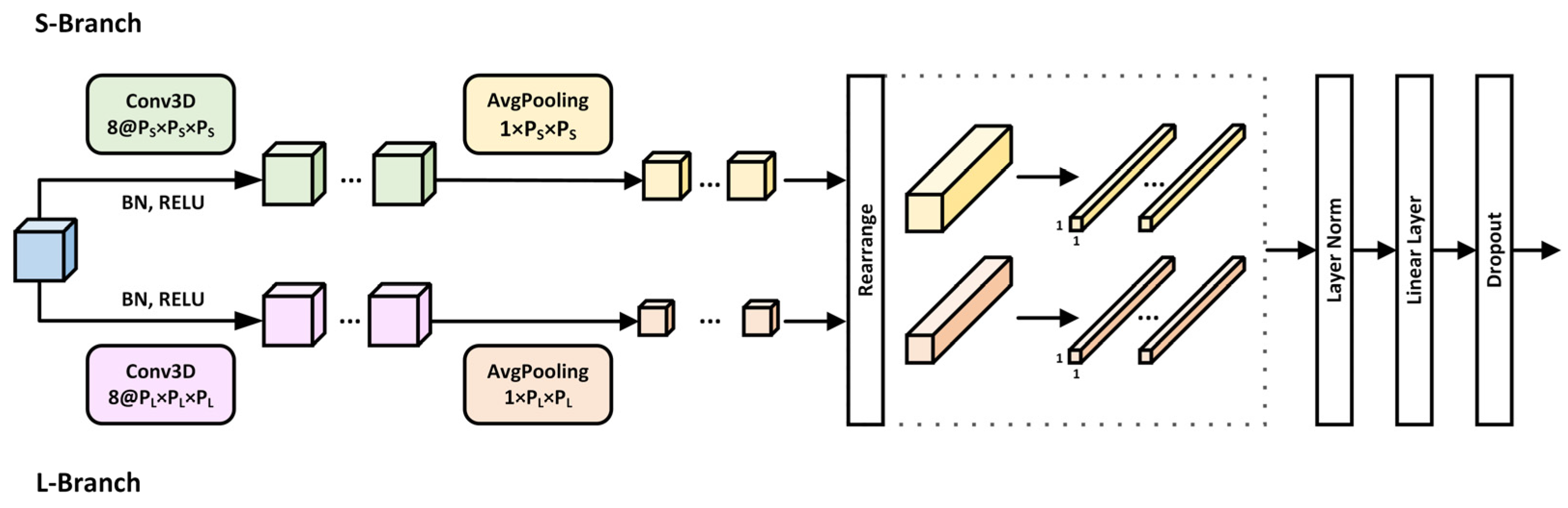
3.2. Multi-Scale Convolutional Information Embedding

To address the issue of key information loss in existing multi-scale methods, limiting the classification performance on imbalanced datasets, we propose a simple and effective multi-scale convolutional information embedding module, as shown in Figure 2. This module is developed with a dual-branch structure, consisting of two 3D convolutional blocks to capture local features and an embedding operation for feature representation. The 3D convolutional blocks are designed based on different patch sizes, enabling the extraction of multi-scale features effectively. The specific descriptions of the MCIE module are given below.

• Three-Dimensional Convolutional Blocks

We construct two branches with different patch sizes ($P_{\mathrm{S}}$ and $P_{\mathrm{L}}$) based on large and small scales. This design not only captures contextual information over a larger range but also facilitates the extraction of fine details. To better extract multi-scale local features, we employ two 3D convolutional blocks. Each block contains a convolutional layer, a batch normalization (BN) layer, a rectified linear unit (ReLU) layer, and a pooling layer. Specifically, we use 8 $P_{\mathrm{S}}\times P_{\mathrm{S}}\times P_{\mathrm{S}}$ and 8 $P_{\mathrm{L}}\times P_{\mathrm{L}}\times P_{\mathrm{L}}$ convolutional kernels covering each patch to enable sufficient extraction of local information at different scales. The BN layer and ReLU layer can effectively mitigate the vanishing gradient problem and accelerate model convergence. The above is specified in Equation (9). Additionally, consistent with the principle of existing transformer-based methods, for an input image of a specific spatial size, we partition it into uniform patches based on the designated patch size. Therefore, we employ a multi-scale pooling operation, i.e., we aggregate local features in pooling sizes of $1\times P_{\mathrm{S}}\times P_{\mathrm{S}}$ and $1\times P_{\mathrm{L}}\times P_{\mathrm{L}}$. This approach replaces direct flattening and prevents the loss of key information. The multi-scale pooling operation not only smooths the data but also retains more spatial and spectral information while reducing the number of parameters, which helps with learning the key features in small target samples, as shown in Equation (10).

$$x_{\mathrm{conv}}=\mathrm{Relu}\left(\mathrm{BN}\left({\mathrm{Conv}}_{P\times P\times P}\left(x_{\mathrm{pca}}\right)\right)\right) , x_{\mathrm{conv}}\in {ℝ}^{C^{\prime }\times D^{\prime }\times H\times W}$$

(9)

$$x_{\mathrm{avg}}={\mathrm{AvgPool}}_{1\times P\times P}\left(x_{\mathrm{conv}}\right) , x_{\mathrm{avg}}\in {ℝ}^{C^{\prime }\times D^{\prime }\times H^{\prime }\times W^{\prime }}$$

(10)

where $P$ represents the patch size, with $P_{\mathrm{S}}$ denoting the small patch size for the S-branch and $P_{\mathrm{L}}$ denoting the large patch size for the L-branch. After pooling, there are $H^{\prime }={\displaystyle \frac{H}{P}}$, $W^{\prime }={\displaystyle \frac{W}{P}}$.

2.

Embedding Operation

The embedding operation is applied to process feature vectors for further deep processing, as shown in Equation (11). As for the specifics, we utilize the rearrange feature to adjust the tensor dimensions, as presented in Equation (12). The layer norm is employed for standardization. The linear layer maps the dimensions, as indicated in Equation (13). To address the potential overfitting caused by class imbalance, we use the dropout to enhance the model’s generalization ability.

$$x_{\mathrm{patch}}={\mathrm{F}}_{\mathrm{embedding}}\left(x_{\mathrm{avg}}\right)$$

(11)

$$\mathrm{Rearrange}: {ℝ}^{C^{\prime }\times D^{\prime }\times H^{\prime }\times W^{\prime }}\to {ℝ}^{\left(H^{\prime }\times W^{\prime }\right)\times \left(C^{\prime }\times D^{\prime }\right)}\to {ℝ}^{N\times E}$$

(12)

$$\mathrm{Linear}: {ℝ}^{N\times E}\to {ℝ}^{N\times F}$$

(13)

where ${\mathrm{F}}_{\mathrm{embedding}}\left( \right)$ represents the embedding operation, $N$ represents the number of patch tokens in each branch, $E$ refers to the dimensionality of the sequence after the rearrange, and $F$ is a custom-defined dimension.

Compared to traditional CNN–transformer hybrid methods [19,45], the proposed MCIE module innovatively introduces a multi-scale pooling operation that differs from standard attention-weighting paradigms before embedding. Instead of directly flattening the input, the module employs average pooling of different sizes to retain more effective spatial and spectral information. Specifically, it not only smooths the data and suppresses noise, enhancing the stability of subsequent spatial–spectral features, but also aggregates local features to mitigate the loss of spatial–spectral and positional information in the embedding process, generating more representative semantic features. As a result, our module enables the network to extract discriminative information even for classes with fewer samples, effectively reducing the misclassification of small target samples in imbalanced datasets.

In summary, the MCIE module could effectively extract local features and help mine more representative information from different scales. It would address the issue in [16], where a single convolution might overlook important details, enhancing the ability of the network to handle complex scenes.

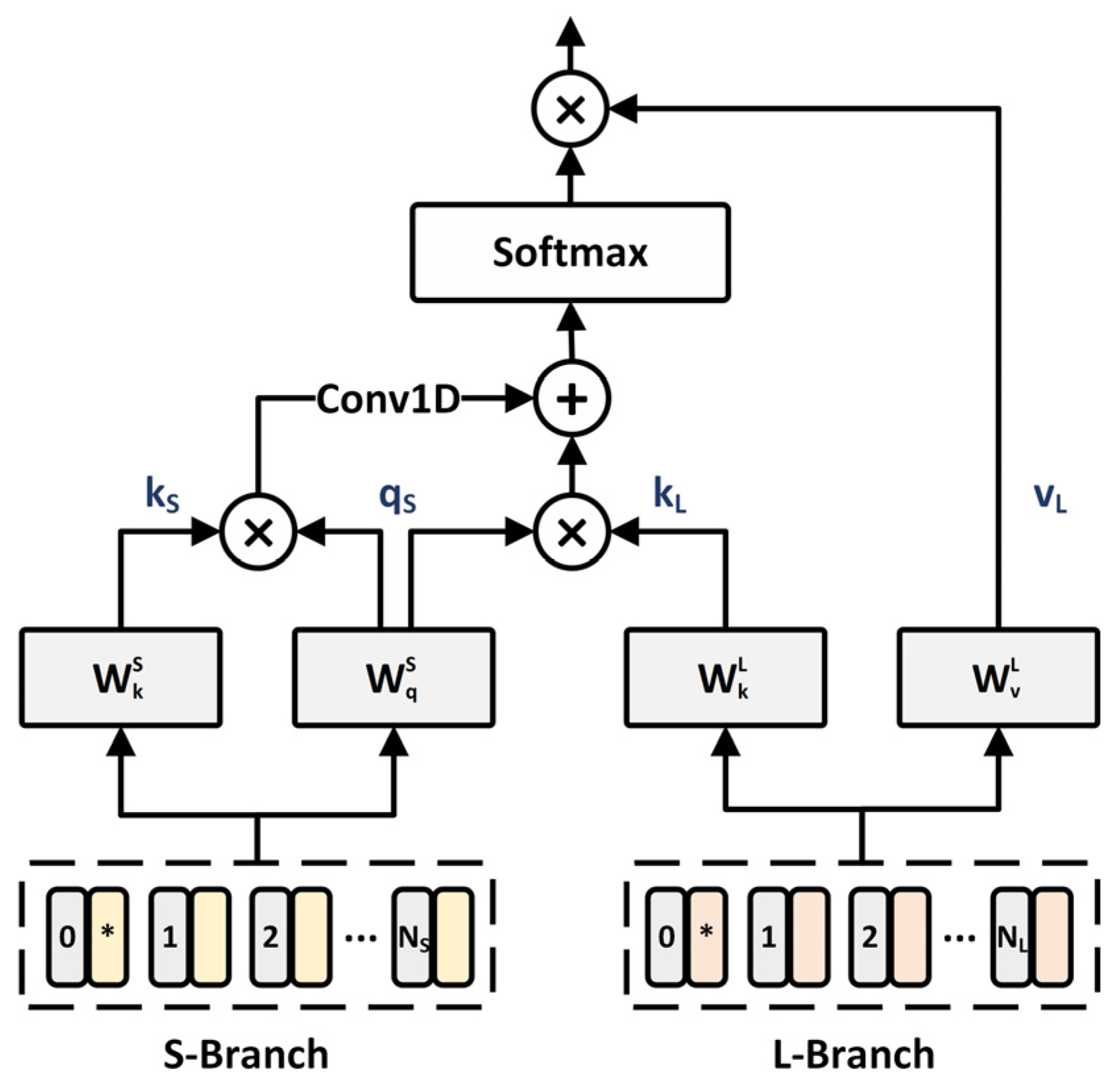
3.3. Dual Aggregated Cross-Attention

An effective feature fusion strategy is crucial for learning multi-scale feature representations. However, existing attention-based feature fusion methods have not yet achieved sufficient cross-scale information fusion [18,23]. To further enhance the feature fusion capability of the model, we designed a dual aggregation cross-attention module. This module adopts a cross-scale interaction strategy to fully achieve information perception between features of different scales, while employing a dual aggregation mechanism to effectively mitigate information loss caused by fusion. The DACA module promotes spatial–spectral feature enhancement and provides high-level semantic information for the entire architecture. Figure 3 illustrates the DACA module for the S-branch.

The DACA module uses the cross-scale interaction strategy, i.e., exchanging the K (key) and V (value) at different scales to achieve deep information fusion. Meanwhile, adopting the dual aggregation mechanism, i.e., utilizing the 1D convolutional layer to adjust the sequence dimensions of the dot products of Q (query) and K (key) for aggregation, mitigating information loss during the attention mechanism’s alternating process. For the above step, given the input sequences $x_{\mathrm{S}}$ and $x_{\mathrm{L}}$ (see Equations (3) and (4)), the computational formula for the S-branch can be expressed as the following:

$$q_{\mathrm{S}}=x_{\mathrm{S}}{W}_q^S,k_{\mathrm{S}}=x_{\mathrm{S}}{W}_k^{\mathrm{S}}$$

(14)

$$k_{\mathrm{L}}=x_{\mathrm{L}}{W}_k^{\mathrm{L}},v_{\mathrm{L}}=x_{\mathrm{L}}{W}_v^{\mathrm{L}}$$

(15)

$$A_{\mathrm{S}}=\mathrm{softmax}\left({\displaystyle \frac{{\mathrm{F}}_{1\mathrm{D}}\left(q_{\mathrm{S}}{k}_{\mathrm{S}}^{\mathrm{T}}\right)+q_{\mathrm{S}}{k}_{\mathrm{L}}^{\mathrm{T}}}{\sqrt{C/h}}}\right)$$

(16)

$$y_{\mathrm{S}}=A_{\mathrm{S}}{v}_{\mathrm{L}}$$

(17)

where $W_q^{\mathrm{S}},W_k^{\mathrm{S}},W_k^{\mathrm{L}},W_v^{\mathrm{L}}\in {ℝ}^{F\times \left(F/h\right)}$ are the learnable parameters, $q_{\mathrm{S}},k_{\mathrm{S}}\in {ℝ}^{\left(1+N_{\mathrm{S}}\right)\times \left(F/h\right)}$ refer to the Q and K of the S-branch, and $k_{\mathrm{L}},v_{\mathrm{L}}\in {ℝ}^{\left(1+N_{\mathrm{L}}\right)\times \left(F/h\right)}$ represent the K and V of the L-branch. $F$ and $h$ represent the embedding dimensions and the number of heads, respectively. ${\mathrm{F}}_{1\mathrm{D}}$( ) is the 1D convolution operation. Given $q_{\mathrm{S}}{k}_{\mathrm{L}}^{\mathrm{T}}\in {ℝ}^{\left(1+N_{\mathrm{S}}\right)\times \left(1+N_{\mathrm{L}}\right)}$ and $q_{\mathrm{S}}{k}_{\mathrm{S}}^{\mathrm{T}}\in {ℝ}^{\left(1+N_{\mathrm{S}}\right)\times \left(1+N_{\mathrm{S}}\right)}$, processing $q_{\mathrm{S}}{k}_{\mathrm{S}}^{\mathrm{T}}$ with ${\mathrm{F}}_{1\mathrm{D}}\left( \right)$ yields ${\mathrm{F}}_{1\mathrm{D}}\left(q_{\mathrm{S}}{k}_{\mathrm{S}}^{\mathrm{T}}\right)\in {ℝ}^{\left(1+N_{\mathrm{S}}\right)\times \left(1+N_{\mathrm{L}}\right)}$ to achieve aggregation. In addition, the L-branch follows the same process.

Our proposed DACA provides a more flexible feature fusion strategy than cross-attention. Cross-attention leverages the class token of one branch to exchange information with the patch tokens of another branch and then maps the information back to the original branch. This fusion strategy facilitates the integration of information from different scales. However, it is essential to ensure the class token has already learned abstract information from its own branch through MHSA before interacting. Meanwhile, this strategy may potentially overlook some important features that exhibit weak self-correlation but are prominent in cross-scale information. Notably, the DACA module eliminates the need for prior attention-aware processing. Instead, it directly interacts with all tokens from different branches, integrating information learned from other branches into the original branch. And the dual-aggregation mechanism is additionally utilized to mitigate the information loss. Therefore, our strategy could enrich the token representations and assure the deeper fusion of different scale features.

The proposed DACA module is able to take full advantage of leveraging the strong complementarity and correlation between features at different scales, improving its capability to understand and model the inherent structure of the data.

4. Experimental Results and Discussion

In this section, we first introduce three widely used datasets for HSI classification and show the training details for the experiments conducted on these datasets, and then we set up five experiments to validate the performance of the proposed MDFFN. For a fair comparison, all experiments are conducted in the same environment.

4.1. Dataset Description

To evaluate the performance of the proposed method, we select three public hyperspectral datasets, namely the Indian Pines, Pavia University, and Houston 2013 datasets. In the experiments, all datasets are divided such that 10% of samples are selected for training and 90% for testing. The detailed information for each of these datasets is provided below.

• Indian Pines Dataset

The Indian Pines (IP) dataset, gathered by the AVIRIS sensor developed by NASA’s Jet Propulsion Laboratory in Pasadena, CA, USA, is an important hyperspectral remote sensing image resource. It consists of 145 × 145 pixels and 220 spectral bands, with 16 vegetation classes, covering the wavelength range of 0.4–2.5 μm. After removing 20 noisy bands, 200 spectral bands are retained for training. The details of the IP dataset are given in

Table 1. Land-cover classes and the sample number of training and testing on Indian Pines dataset.

No.	Class	Training	Testing
1	Alfalfa	5	41
2	Corn—no till	143	1285
3	Corn—min till	83	747
4	Corn	24	213
5	Grass—pasture	48	435
6	Grass—trees	73	657
7	Grass—pasture–mowed	3	25
8	Hay—windrowed	48	430
9	Oats	2	18
10	Soybean—no till	97	875
11	Soybean—min till	245	2210
12	Soybean—clean	59	534
13	Wheat	20	185
14	Woods	126	1139
15	Building—grass-trees-drives	39	347
16	Stone—steel-towers	9	84
Total		1024	9225

. It is worth mentioning that this dataset has limited samples and an imbalanced distribution of various classes in quantity. For instance, the eleventh class contains 2455 samples, while the ninth class contains only 20 samples (with a ratio of 1:122). This imbalanced dataset may lead to poor model generalization and potentially cause overfitting, posing a challenge for classification.

2.

Pavia University Dataset

The Pavia University (PU) dataset was acquired by the ROSIS sensor over Pavia in Northern Italy. The sensor was developed jointly by Dornier Satellite Systems (DSS, former MBB), GKSS Research Centre Geesthacht, and the German Aerospace Center (DLR). This dataset includes 610 × 340 pixels and 115 spectral bands, covering the wavelength range of 0.43–0.86 μm. The dataset contains nine land-cover classes. After removing 12 noisy bands, 103 spectral bands are retained for training. The details of the PU dataset are shown in

Table 2. Land-cover classes and the sample numbers for training and testing in Pavia University dataset.

No.	Class	Training	Testing
1	Asphalt	663	5968
2	Meadows	1865	16,784
3	Gravel	210	1889
4	Trees	306	2758
5	Painted metal sheets	134	1211
6	Bare soil	503	4526
7	Bitumen	133	1197
8	Self-blocking bricks	368	3314
9	Shadows	95	852
Total		4277	38,499

. The distribution of the land-cover sample numbers is also imbalanced, with the ninth class having 947 samples and the second class having 18,649 samples (with a ratio of 1:19). Nevertheless, compared to the IP dataset, the sample numbers in the PU dataset are more abundant.

3.

Houston 2013 Dataset

The Houston 2013 dataset was acquired with the ITRES CASI-1500 sensor, developed by ITRES Research Limited in Calgary, AB, Canada, capturing remote sensing images of Houston and its surrounding rural areas. It consists of 349 × 1905 pixels and 144 spectral bands. The wavelength range is 0.38–1.05 μm. The dataset includes 15 challenging land-cover classes, and the details are shown in

Table 3. Land-cover classes and the sample numbers of training and testing on Houston 2013 dataset.

No.	Class	Training	Testing
1	Healthy grass	125	1126
2	Stressed grass	125	1129
3	Synthetic grass	70	627
4	Tree	124	1120
5	Soil	124	1118
6	Water	33	292
7	Residential	127	1141
8	Commercial	124	1120
9	Road	125	1127
10	Highway	123	1104
11	Railway	123	1112
12	Parking lot 1	123	1110
13	Parking lot 2	47	422
14	Tennis court	43	385
15	Running track	66	594
Total		1502	13,527

.

4.2. Experimental Setup

• Training details: For a fair comparison, all experiments are conducted on an Intel^® Xeon^® Platinum 8358P CPU @ 2.60GHz processor and an NVIDIA GeForce RTX 3090 GPU (24GB) (NVIDIA Corporation, Santa Clara, CA, USA), utilizing the PyTorch 1.11 framework with Python 3.8. To minimize the errors in the experiments, all results are the average and standard deviation of 10 independent runs. For model training, we utilize the Adam optimizer to learn the weights, set the batch size to 100 and the learning rate to 1 × 10⁻⁴. To ensure the model is sufficiently trained and performing at its best, we run the model for 100 epochs.
• Evaluation metrics: We employ three widely used metrics to evaluate the classification performance of different models: overall accuracy (OA), average accuracy (AA), and kappa coefficient (Kappa). Additionally, to facilitate a more intuitive comparison among the models, we visualize the classification results for qualitative analysis.
• Experimental details: In order to more rationally validate the performance of the proposed MDFFN method, we set up five detailed experiments.

  (a)

  Comparison with state-of-the-art methods: we compare the proposed MDFFN model with representative baseline methods and state-of-the-art backbone methods for validating the performance.

  (b)

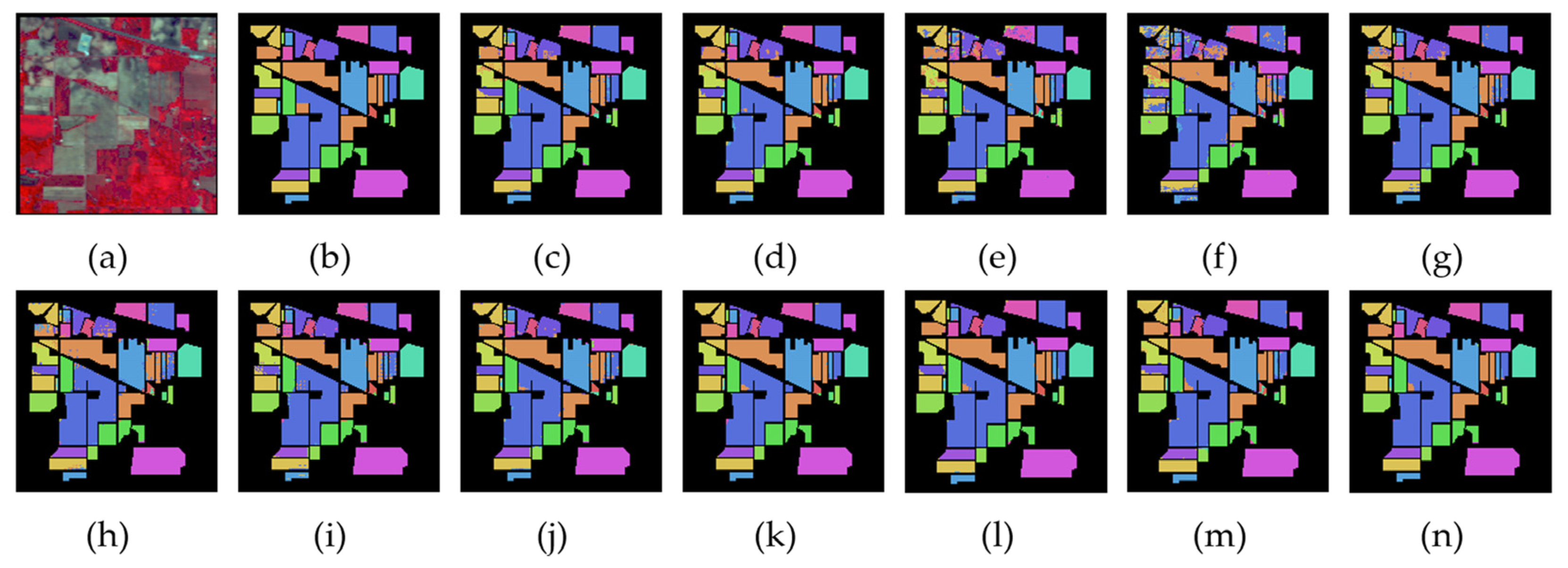
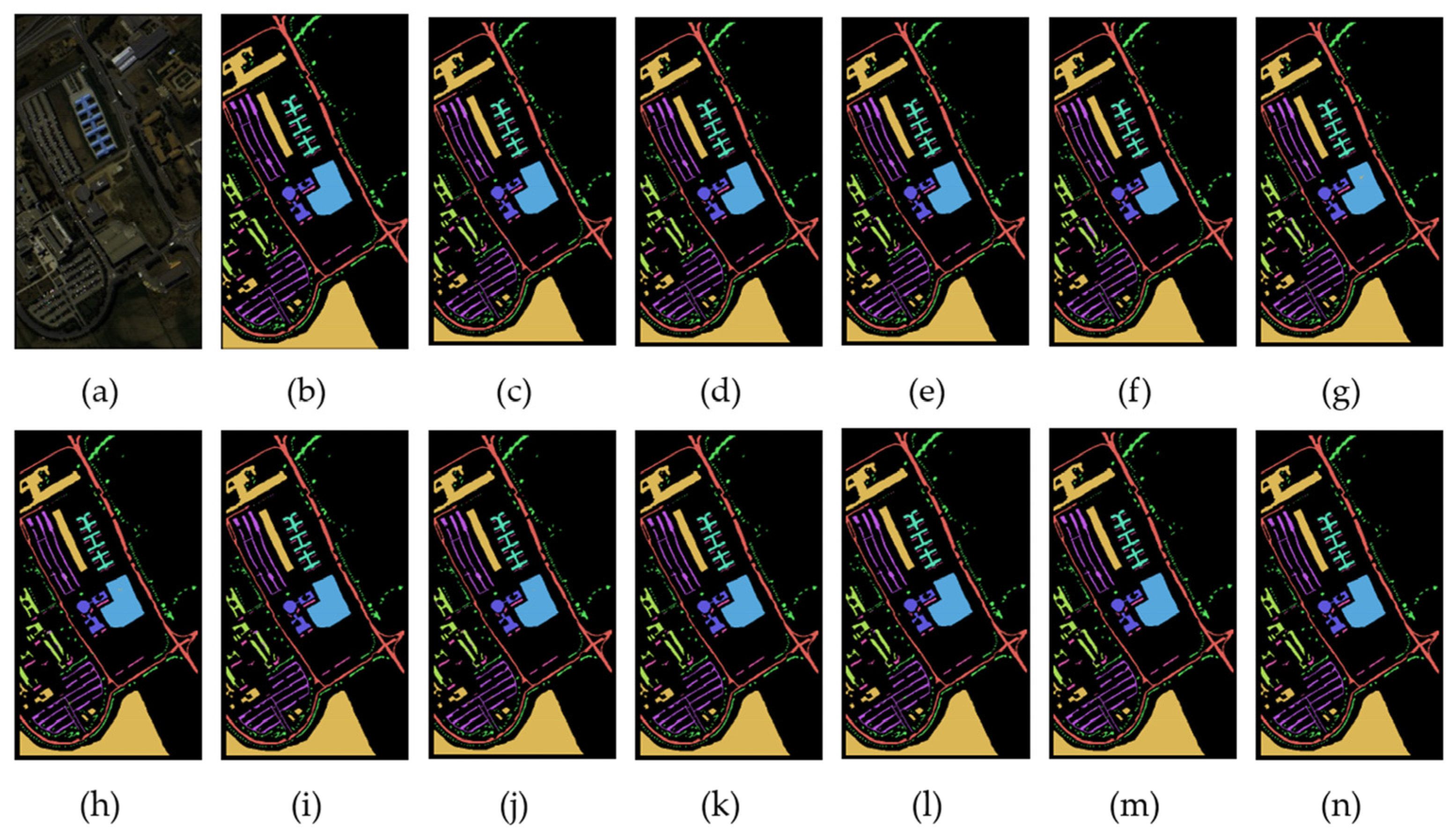
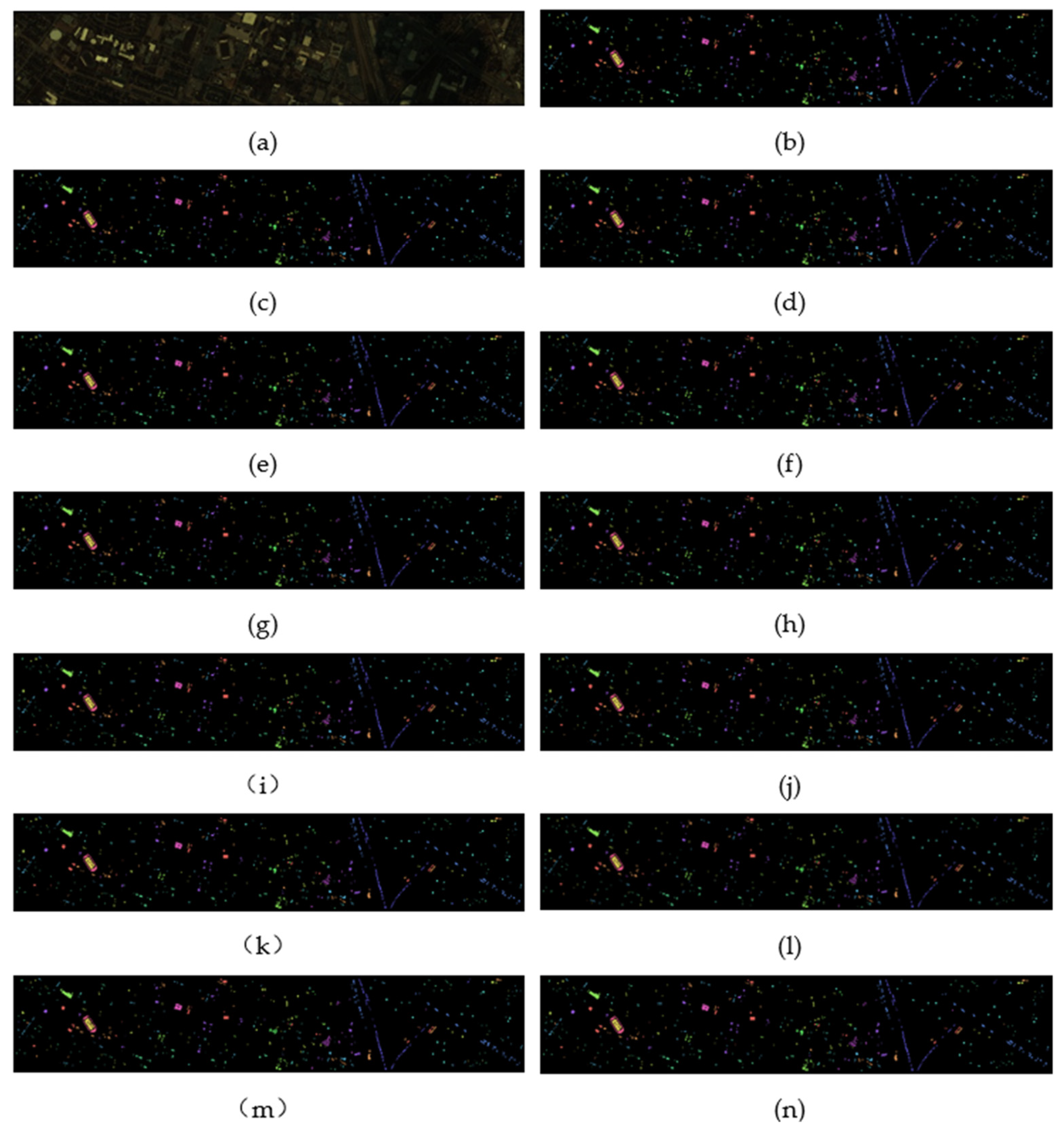
  Visual evaluation: the experimental results are visualized to provide a clear and intuitive demonstration of the progressiveness of the model.

  (c)

  Efficiency analysis: we quantitatively evaluate the computational efficiency of the proposed method by comparing parameter counts, FLOPs, training time, and testing time with state-of-the-art methods.

  (d)

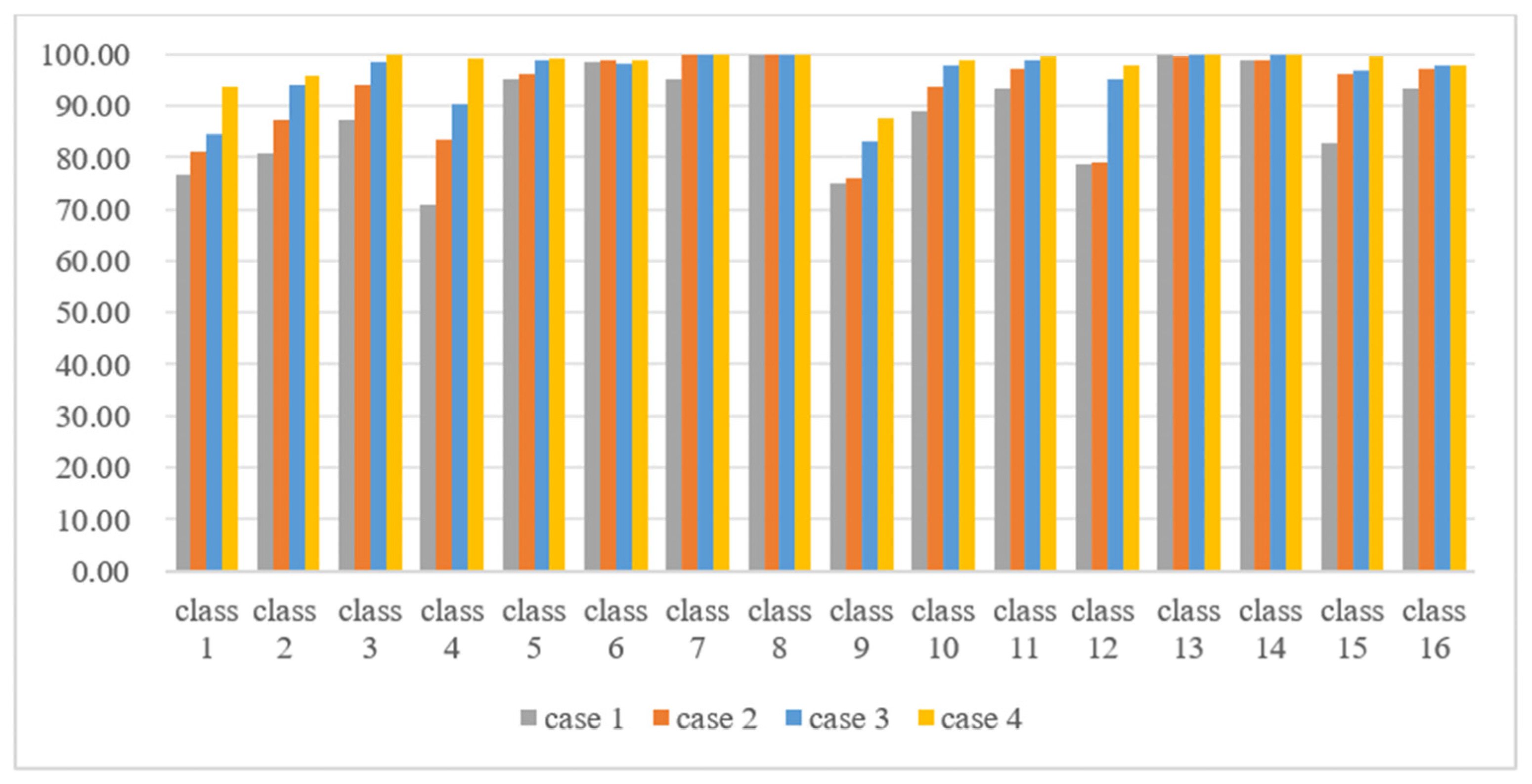
  Ablation experiments: ablation experiments are conducted to verify the effectiveness of the MCIE and DACA modules in the network.

  (e)

  Parameter sensitivity experiments: parameter sensitivity experiments are set up to evaluate the performance of MDFFN with different combinations of S-branch size and L-branch size, different depths of the multi-scale transformer, and different proportions of training samples on the experimental results.

• Comparison with state-of-the-art backbone networks: To validate the performance of the proposed MDFFN, we selected several representative baseline methods and state-of-the-art backbone methods, including CNN-based methods (i.e., 2D-CNN [46], 3D-CNN [46], HybridSN [33], and M3D-DCNN [36]), transformer-based methods (i.e., ViT [16], CrossViT [18], DeepViT [17], and SpectralFormer [34]), as well as CNN–transformer hybrid-based methods (i.e., SSFTT [19], morphFormer [20], and MSNAT [22]). In order to make a reasonable comparison, the experiments basically maintain consistent parameter settings. Regarding parameters, we set the spatial size of morphFormer and MSNAT to 11 × 11, and the other methods to 15 × 15. For the patch size, ViT and DeepViT are 3, while for the multi-scale methods CrossViT and MDFFN, the small branch is set to 3 and the large branch to 5. The depth of ViT, CrossViT, DeepViT, and MDFFN is set to 3, and the dimension is set to 512. Otherwise, all other parameters not listed are set to their default values. More details can be found in the original papers.

4.3. Results and Analysis

4.3.1. Comparison with State-of-the-Art Methods

The quantitative analysis results on the three datasets are displayed in

Table 4. Comparison results on the IP dataset.

Class	CNN-Based Methods				Transformer-Based Methods				CNN-Transformer Hybrid-Based Methods
	2D-CNN	3D-CNN	HybridSN	M3D-DCNN	ViT	CrossViT	DeepViT	SpectralFormer	SSFTT	morphFormer	MSNAT	MDFFN
1	42.68 ± 7.50	79.76 ± 8.93	24.39 ± 10.12	32.68 ± 12.20	80.73 ± 9.66	70.24 ± 9.80	89.02 ± 2.73	73.41 ± 4.15	94.15 ± 5.89	96.59 ± 5.79	71.46 ± 12.91	93.90 ± 2.50
2	90.05 ± 0.96	91.05 ± 1.15	90.29 ± 4.47	81.73 ± 2.24	87.22 ± 0.92	85.75 ± 0.83	87.99 ± 1.01	91.23 ± 0.47	95.14 ± 0.39	94.44 ± 0.63	93.81 ± 2.11	95.82 ± 0.21
3	95.03 ± 1.42	93.98 ± 1.53	92.37 ± 5.99	65.92 ± 9.88	92.77 ± 1.36	93.64 ± 1.29	92.78 ± 1.49	96.12 ± 0.49	99.59 ± 0.40	98.18 ± 0.64	99.09 ± 0.91	99.91 ± 0.19
4	78.64 ± 3.06	75.73 ± 8.70	63.66 ± 15.22	30.19 ± 10.62	77.28 ± 5.88	89.01 ± 2.79	90.05 ± 2.39	91.69 ± 2.75	100.00 ± 0.00	99.20 ± 1.09	95.73 ± 3.16	99.20 ± 0.37
5	95.29 ± 1.43	98.09 ± 1.31	94.76 ± 1.35	91.08 ± 1.93	96.14 ± 0.85	96.16 ± 0.73	96.90 ± 0.34	96.94 ± 0.50	99.52 ± 0.30	99.15 ± 0.81	95.24 ± 1.10	99.38 ± 0.40
6	98.40 ± 0.51	97.93 ± 0.49	97.78 ± 3.40	96.41 ± 1.68	99.24 ± 0.34	98.58 ± 0.38	98.25 ± 0.64	99.07 ± 0.38	99.73 ± 0.40	99.36 ± 0.59	97.78 ± 1.19	99.01 ± 0.27
7	34.40 ± 11.48	97.20 ± 5.08	40.00 ± 24.98	30.40 ± 19.03	97.60 ± 2.65	92.00 ± 7.16	64.40 ± 12.58	95.20 ± 5.00	78.40 ± 28.41	100.00 ± 0.00	94.40 ± 6.97	100.00 ± 0.00
8	99.93 ± 0.15	99.51 ± 0.49	99.91 ± 0.15	99.74 ± 0.28	99.98 ± 0.07	100.00 ± 0.00	100.00 ± 0.00	99.88 ± 0.21	100.00 ± 0.00	99.98 ± 0.07	99.93 ± 0.15	99.95 ± 0.09
9	13.33 ± 3.69	58.89 ± 16.14	34.44 ± 10.48	28.89 ± 24.70	60.00 ± 12.37	80.00 ± 11.97	39.44 ± 9.44	50.00 ± 8.61	36.11 ± 14.96	70.56 ± 16.11	48.89 ± 19.85	87.78 ± 4.16
10	93.25 ± 1.22	94.39 ± 2.00	94.19 ± 2.11	81.82 ± 3.28	94.69 ± 0.85	91.99 ± 1.00	92.77 ± 1.33	94.59 ± 0.71	98.75 ± 0.63	98.56 ± 0.84	97.25 ± 1.24	99.01 ± 0.40
11	98.11 ± 0.34	97.38 ± 0.69	97.97 ± 0.86	93.92 ± 1.12	96.58 ± 1.17	96.36 ± 0.68	97.03 ± 0.42	97.69 ± 0.36	99.47 ± 0.21	99.06 ± 0.40	98.05 ± 1.06	99.47 ± 0.17
12	79.48 ± 3.38	84.61 ± 3.61	70.86 ± 18.74	59.10 ± 10.20	79.74 ± 3.48	77.96 ± 2.07	83.41 ± 2.86	93.65 ± 1.37	97.98 ± 0.61	95.34 ± 1.24	96.67 ± 1.40	97.72 ± 0.38
13	98.32 ± 1.04	98.38 ± 1.57	93.57 ± 10.55	94.97 ± 3.71	100.00 ± 0.00	99.73 ± 0.27	97.51 ± 1.80	97.73 ± 0.99	99.62 ± 0.49	98.65 ± 0.97	99.24 ± 0.69	100.00 ± 0.00
14	99.71 ± 0.17	99.41 ± 0.70	99.65 ± 0.29	97.39 ± 1.14	99.27 ± 0.27	98.72 ± 0.23	98.36 ± 0.36	99.30 ± 0.41	99.97 ± 0.04	99.95 ± 0.07	99.51 ± 0.26	99.99 ± 0.03
15	95.68 ± 2.99	95.53 ± 2.07	55.62 ± 22.05	97.39 ± 1.14	93.20 ± 1.69	97.03 ± 0.78	93.11 ± 1.52	94.24 ± 1.91	99.08 ± 1.11	98.50 ± 0.82	95.79 ± 2.05	99.65 ± 0.28
16	75.00 ± 2.77	84.40 ± 4.75	60.60 ± 33.20	53.45 ± 17.40	96.07 ± 3.11	97.86 ± 1.39	82.62 ± 6.63	96.43 ± 2.71	88.33 ± 3.40	96.55 ± 1.95	91.67 ± 6.00	97.98 ± 0.76
OA (%)	94.04 ± 0.34	94.80 ± 0.78	91.23 ± 3.39	83.57 ± 1.86	93.82 ± 0.41	93.57 ± 0.23	93.95 ± 0.36	96.01 ± 0.14	98.52 ± 0.15	98.15 ± 0.21	97.10 ± 0.81	98.85 ± 0.09
AA (%)	80.46 ± 1.03	90.39 ± 1.76	75.63 ± 7.21	68.10 ± 4.25	90.66 ± 1.38	91.56 ± 1.02	87.73 ± 1.19	91.70 ± 0.88	92.86 ± 2.33	96.50 ± 1.15	92.16 ± 2.22	98.05 ± 0.32
Kappa (%)	93.18 ± 0.39	94.06 ± 0.90	89.95 ± 3.91	81.03 ± 2.18	92.94 ± 0.46	92.65 ± 0.26	93.09 ± 0.42	95.45 ± 0.16	98.32 ± 0.17	97.89 ± 0.23	96.70 ± 0.92	98.69 ± 0.10

The bold entities indicate the highest value.

,

Table 5. Comparison results on the PU dataset.

Class	CNN-Based Methods				Transformer-Based Methods				CNN-Transformer Hybrid-Based Methods
	2D-CNN	3D-CNN	HybridSN	M3D-DCNN	ViT	CrossViT	DeepViT	SpectralFormer	SSFTT	morphFormer	MSNAT	MDFFN
1	99.52 ± 0.11	99.52 ± 0.18	99.48 ± 0.68	99.14 ± 0.43	99.38 ± 0.19	99.40 ± 0.19	99.79 ± 0.08	99.63 ± 0.15	99.94 ± 0.05	99.91 ± 0.05	99.89 ± 0.14	99.99 ± 0.02
2	100.00 ± 0.00	99.98 ± 0.01	100.00 ± 0.01	99.95 ± 0.03	99.98 ± 0.01	99.99 ± 0.00	99.98 ± 0.01	99.98 ± 0.01	99.99 ± 0.01	99.99 ± 0.01	99.99 ± 0.01	100.00 ± 0.00
3	95.80 ± 0.88	95.98 ± 0.98	97.20 ± 1.00	91.20 ± 0.93	93.01 ± 1.29	95.85 ± 0.52	95.64 ± 0.94	95.99 ± 0.87	99.49 ± 0.16	98.54 ± 0.48	98.34 ± 1.33	99.70 ± 0.27
4	98.86 ± 0.13	98.85 ± 0.43	98.76 ± 1.12	98.13 ± 0.46	99.65 ± 0.14	98.98 ± 0.18	98.42 ± 0.40	99.19 ± 0.19	98.61 ± 0.24	98.60 ± 0.34	99.72 ± 0.13	99.85 ± 0.06
5	99.90 ± 0.09	99.84 ± 0.15	99.70 ± 0.63	99.93 ± 0.20	100.00 ± 0.00	100.00 ± 0.00	99.88 ± 0.12	99.98 ± 0.05	99.97 ± 0.08	99.97 ± 0.07	99.99 ± 0.02	100.00 ± 0.00
6	100.00 ± 0.00	99.98 ± 0.03	99.99 ± 0.01	99.75 ± 0.26	99.59 ± 0.16	99.83 ± 0.08	99.96 ± 0.04	99.85 ± 0.08	100.00 ± 0.00	100.00 ± 0.00	99.99 ± 0.04	100.00 ± 0.00
7	99.74 ± 0.28	99.82 ± 0.26	98.65 ± 3.49	98.72 ± 0.79	99.97 ± 0.05	99.94 ± 0.07	99.84 ± 0.26	99.87 ± 0.23	100.00 ± 0.00	100.00 ± 0.00	99.76 ± 0.34	100.00 ± 0.00
8	97.36 ± 0.72	98.22 ± 0.96	96.40 ± 2.63	95.00 ± 0.78	98.37 ± 0.30	97.40 ± 0.43	98.96 ± 0.28	97.91 ± 0.50	98.77 ± 0.45	98.82 ± 0.21	99.19 ± 0.46	99.86 ± 0.10
9	97.52 ± 0.65	96.10 ± 1.42	94.42 ± 4.89	95.31 ± 1.52	100.00 ± 0.00	99.84 ± 0.16	99.31 ± 0.60	98.37 ± 0.61	97.23 ± 0.32	97.56 ± 0.49	99.82 ± 0.39	100.00 ± 0.00
OA (%)	99.34 ± 0.09	99.39 ± 0.12	99.21 ± 0.48	98.67 ± 0.17	99.34 ± 0.07	99.38 ± 0.04	99.51 ± 0.06	99.44 ± 0.06	99.69 ± 0.04	99.65 ± 0.06	99.80 ± 0.14	99.96 ± 0.02
AA (%)	98.74 ± 0.18	98.70 ± 0.27	98.29 ± 1.13	97.46 ± 0.33	98.88 ± 0.13	99.02 ± 0.06	99.09 ± 0.11	98.97 ± 0.13	99.33 ± 0.04	99.26 ± 0.12	99.63 ± 0.29	99.93 ± 0.04
Kappa (%)	99.13 ± 0.12	99.19 ± 0.16	98.95 ± 0.63	98.24 ± 0.22	99.12 ± 0.09	99.18 ± 0.05	99.36 ± 0.07	99.26 ± 0.07	99.59 ± 0.05	99.54 ± 0.07	99.73 ± 0.19	99.95 ± 0.02

The bold entities indicate the highest value.

and

Table 6. Comparison results on the Houston 2013 dataset.

Class	CNN-Based Methods				Transformer-Based Methods				CNN-Transformer Hybrid-Based Methods
	2D-CNN	3D-CNN	HybridSN	M3D-DCNN	ViT	CrossViT	DeepViT	SpectralFormer	SSFTT	morphFormer	MSNAT	MDFFN
1	95.97 ± 2.17	98.39 ± 0.68	99.25 ± 0.36	96.70 ± 1.06	97.08 ± 0.76	98.05 ± 1.20	98.53 ± 0.94	99.77 ± 0.24	96.58 ± 1.86	98.57 ± 0.64	97.80 ± 1.02	99.25 ± 0.37
2	99.39 ± 0.42	99.42 ± 0.62	99.77 ± 0.16	99.62 ± 0.20	99.76 ± 0.06	99.86 ± 0.06	99.81 ± 0.29	99.89 ± 0.07	99.19 ± 0.52	99.17 ± 0.34	99.65 ± 0.16	99.89 ± 0.04
3	99.79 ± 0.07	99.98 ± 0.05	99.98 ± 0.05	99.94 ± 0.08	100.00 ± 0.00	99.92 ± 0.08	99.82 ± 0.13	100.00 ± 0.00	99.62 ± 0.11	99.78 ± 0.15	99.98 ± 0.05	99.87 ± 0.06
4	97.79 ± 0.75	96.42 ± 1.51	97.59 ± 1.24	96.88 ± 1.69	99.04 ± 0.44	98.88 ± 0.49	97.89 ± 0.84	98.56 ± 0.50	97.27 ± 1.00	96.81 ± 1.45	99.50 ± 0.86	99.29 ± 0.55
5	99.95 ± 0.08	99.79 ± 0.33	100.00 ± 0.00	99.73 ± 0.40	100.00 ± 0.00	100.00 ± 0.00	100.00 ± 0.00	99.91 ± 0.27	100.00 ± 0.00	99.99 ± 0.03	99.99 ± 0.03	100.00 ± 0.00
6	90.65 ± 3.35	96.61 ± 1.73	98.29 ± 2.16	93.15 ± 2.56	99.97 ± 0.10	99.93 ± 0.21	99.42 ± 0.49	99.76 ± 0.43	99.76 ± 0.41	99.90 ± 0.31	99.01 ± 1.42	100.00 ± 0.00
7	93.81 ± 1.92	95.07 ± 0.98	94.77 ± 1.61	93.19 ± 1.96	97.43 ± 0.56	96.93 ± 0.59	96.26 ± 0.57	96.61 ± 0.61	96.03 ± 1.20	95.03 ± 0.84	97.03 ± 1.04	98.20 ± 0.44
8	90.45 ± 3.96	95.01 ± 1.54	97.66 ± 0.82	94.10 ± 0.99	97.45 ± 0.67	97.62 ± 0.46	98.02 ± 0.40	97.75 ± 0.60	95.37 ± 1.25	96.95 ± 1.17	95.49 ± 1.27	98.18 ± 0.74
9	92.83 ± 2.37	95.97 ± 2.31	97.08 ± 1.26	93.01 ± 1.96	95.47 ± 0.94	97.24 ± 0.76	97.95 ± 0.99	97.83 ± 0.75	97.97 ± 1.65	97.66 ± 1.44	94.08 ± 2.22	98.97 ± 0.39
10	99.36 ± 0.62	99.48 ± 0.44	99.68 ± 0.27	98.31 ± 1.74	99.57 ± 0.29	99.66 ± 0.22	99.83 ± 0.14	99.66 ± 0.28	99.81 ± 0.41	99.77 ± 0.24	99.81 ± 0.17	100.00 ± 0.00
11	96.91 ± 0.77	99.10 ± 0.54	99.81 ± 0.19	98.71 ± 0.87	99.90 ± 0.14	99.99 ± 0.03	99.98 ± 0.04	99.54 ± 0.29	99.73 ± 0.39	99.18 ± 0.53	97.37 ± 2.59	100.00 ± 0.00
12	97.95 ± 1.51	98.77 ± 0.65	99.39 ± 0.18	98.70 ± 0.30	98.75 ± 0.34	99.04 ± 0.13	98.86 ± 0.23	99.19 ± 0.13	99.50 ± 0.14	99.45 ± 0.44	99.15 ± 0.28	99.61 ± 0.04
13	85.92 ± 2.74	88.15 ± 2.92	90.50 ± 4.56	79.27 ± 5.44	81.59 ± 2.80	84.79 ± 3.04	89.27 ± 1.89	94.41 ± 1.06	92.37 ± 0.83	93.06 ± 2.91	95.05 ± 1.34	99.10 ± 0.49
14	99.51 ± 0.34	99.22 ± 0.94	99.97 ± 0.08	99.95 ± 0.16	100.00 ± 0.00	100.00 ± 0.00	100.00 ± 0.00	99.82 ± 0.17	100.00 ± 0.00	100.00 ± 0.00	98.99 ± 1.04	100.00 ± 0.00
15	100.00 ± 0.00	100.00 ± 0.00	99.98 ± 0.05	100.00 ± 0.00	100.00 ± 0.00	99.83 ± 0.18	99.48 ± 0.24	100.00 ± 0.00	100.00 ± 0.00	99.95 ± 0.11	99.95 ± 0.11	100.00 ± 0.00
OA (%)	96.38 ± 0.54	97.66 ± 0.40	98.41 ± 0.30	96.62 ± 0.55	98.13 ± 0.12	98.45 ± 0.19	98.55 ± 0.20	98.88 ± 0.12	98.19 ± 0.27	98.32 ± 0.35	98.12 ± 0.34	99.42 ± 0.07
AA (%)	96.02 ± 0.54	97.43 ± 0.37	98.25 ± 0.50	96.08 ± 0.65	97.73 ± 0.19	98.12 ± 0.26	98.34 ± 0.22	98.85 ± 0.11	98.21 ± 0.22	98.35 ± 0.39	98.19 ± 0.29	99.49 ± 0.07
Kappa (%)	96.08 ± 0.59	97.47 ± 0.44	98.28 ± 0.33	96.34 ± 0.60	97.98 ± 0.12	98.33 ± 0.20	98.43 ± 0.22	98.79 ± 0.13	98.05 ± 0.29	98.18 ± 0.38	97.97 ± 0.37	99.37 ± 0.08

The bold entities indicate the highest value.

, showing that the proposed MDFFN demonstrates considerable advantages compared to the state-of-the-art backbone methods.

• The performance in the overall method

Observation of Table 4, Table 5 and Table 6 reveals that our MDFFN obtains the best OA, AA, and Kappa with relatively low standard deviation on different datasets compared to existing methods.

Compared to CNN-based methods, ours achieves OA of 99.96% ± 0.02 and 99.42% ± 0.07 on the PU dataset and Houston 2013 dataset, respectively, and AA of 98.05% ± 0.32 on the IP dataset. In contrast, the OA for 2D-CNN and 3D-CNN are 99.34% ± 0.09 and 99.39% ± 0.12 on the PU dataset, HybridSN and M3D-DCNN are 98.41% ± 0.30 and 96.62% ± 0.55 on Houston 2013 dataset. In Table 4, it can be seen that our method is 22.42% and 29.95% higher compared to HybridSN and M3D-DCNN. The possible reason is that the IP dataset has a more concentrated distribution of the same type of pixels compared to other datasets. The methods with the smaller convolution kernels have limited receptive fields, ignoring important global information in the feature maps.

Compared to transformer-based methods, the proposed MDFFN also obtains the best performance, with its OA on the PU dataset surpassing ViT, CrossViT, DeepViT, and SpectralFormer by 0.62%, 0.58%, 0.45%, and 0.52%, respectively. This is due to the fact that the transformer-based methods are still deficient in capturing local information, although they have advantages in handling long-range dependencies.

Compared to other CNN-transformer hybrid-based methods, SSFTT (99.69% ± 0.04), morphFormer (99.65% ± 0.06), and MSNAT (99.80% ± 0.14) show relatively better performance on the PU dataset. These approaches are effective in combining the benefits of CNN in local feature extraction with the advantages of transformer in dealing with long-range dependencies, enhancing the ability of the network to handle complex scenes. Notably, our MDFFN indicates more favorable results, with the OA improved by 0.27%, 0.31%, and 0.16%, and Kappa improved by 0.36%, 0.41%, and 0.22%, respectively. The possible reason is that SSFTT and morphFormer directly flatten the features obtained from convolution, resulting in the loss of some key information. And MSNAT simply fuses multi-scale features by parallel summation, which overlooks the differences among the various features. For our approach, combining the MCIE module with the DACA module shows superiority in fine feature extraction and deep feature fusion. Consequently, MDFFN could adequately exploit the abundant spatial–spectral features in HSI, enhancing the model’s performance and robustness.

2.

The performance in multi-scale feature extraction and fusion

On the Houston 2013 dataset, the OA is 99.42% ± 0.07 and the Kappa is 99.37% ± 0.08 for MDFFN, whose OA outperforms the single-scale methods such as ViT (98.13% ± 0.12), DeepViT (98.55% ± 0.20), and SSFTT (98.19% ± 0.27). While single-scale approaches typically capture limited information, our method employs the multi-scale strategy to enable a more comprehensive extraction of spatial and spectral features in HSI. Meanwhile, MDFFN outperforms the multi-scale methods such as CrossViT, morphFormer, and MSNAT by 0.97%, 1.1%, and 1.3%, respectively, in terms of OA on the Houston 2013 dataset, and outperforms the best-performing MSNAT by 0.16% on the PU dataset. The above results demonstrate the potential of MDFFN in multi-scale local feature extraction. Unlike the better-performing CrossViT that directly uses a flattening operation, MDFFN utilizes the MCIE module to retain more effective spatial and spectral information, highlighting discriminative features. (See more explanations about the performance of the MCIE module in Section 4.3.4 for Ablation Experiments).

Observing Table 4, compared with the methods using feature fusion, MDFFN improves OA by 2.84% and Kappa by 3.24% compared to SpectralFormer, and the AA shows improvements of 6.49% and 1.55% over CrossViT and morphFormer based on attention mechanism, respectively, on the IP dataset. Similarly, our method is superior to the above across all metrics on other datasets. This demonstrates that MDFFN exhibits superior feature fusion capability, which could facilitate further spatial–spectral feature enhancement by utilizing the DACA module for deep multi-scale feature fusion. (See more explanations about the performance of the DACA module in Section 4.3.4 for Ablation Experiments).

In conclusion, our proposed MDFFN utilizes the MCIE module to extract multi-scale spatial–spectral features and adopts the DACA module to fully realize the information perception between different features, which can better solve the multi-scale challenges in different land-cover types.

3.

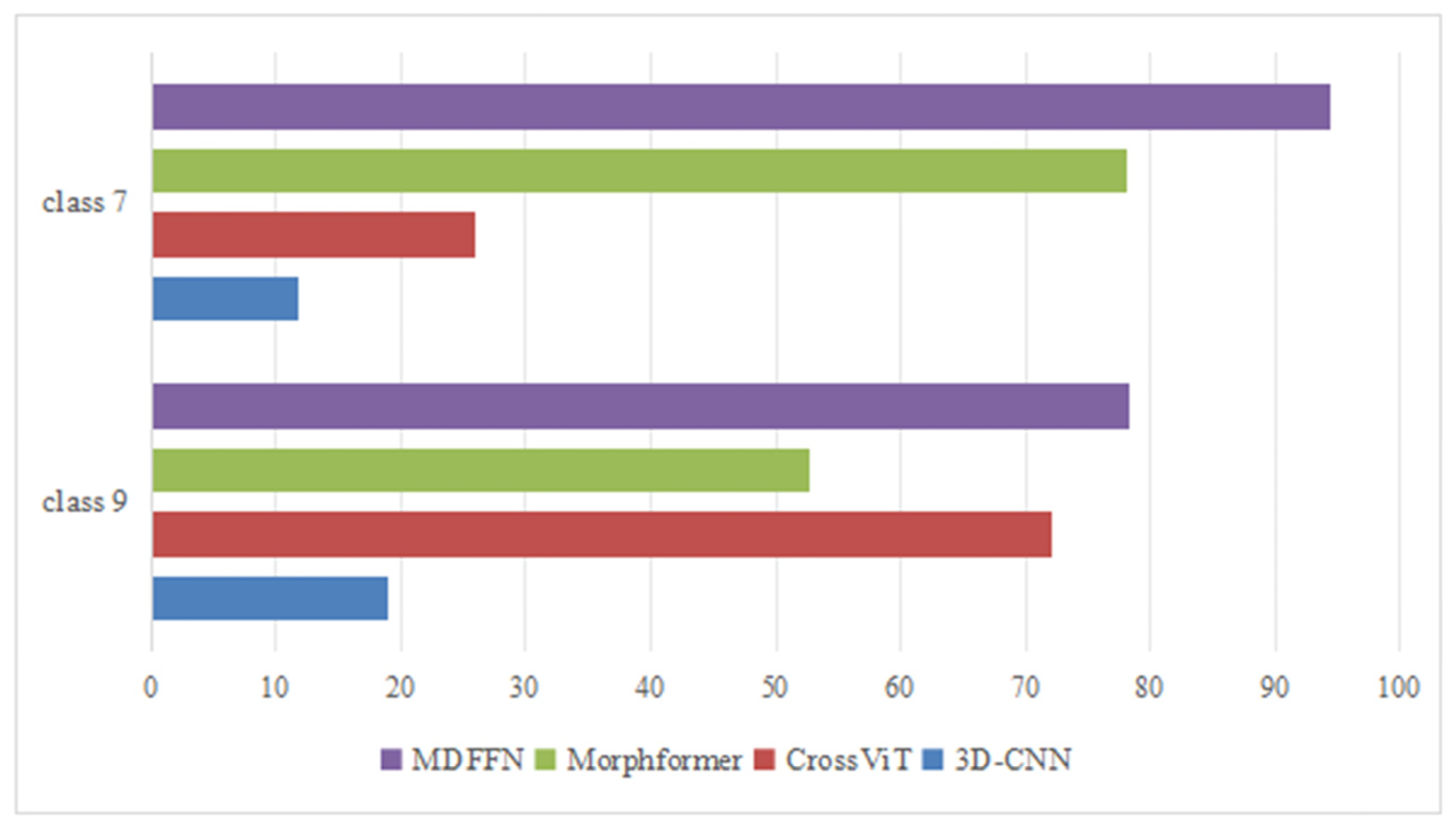
The performance on imbalanced datasets

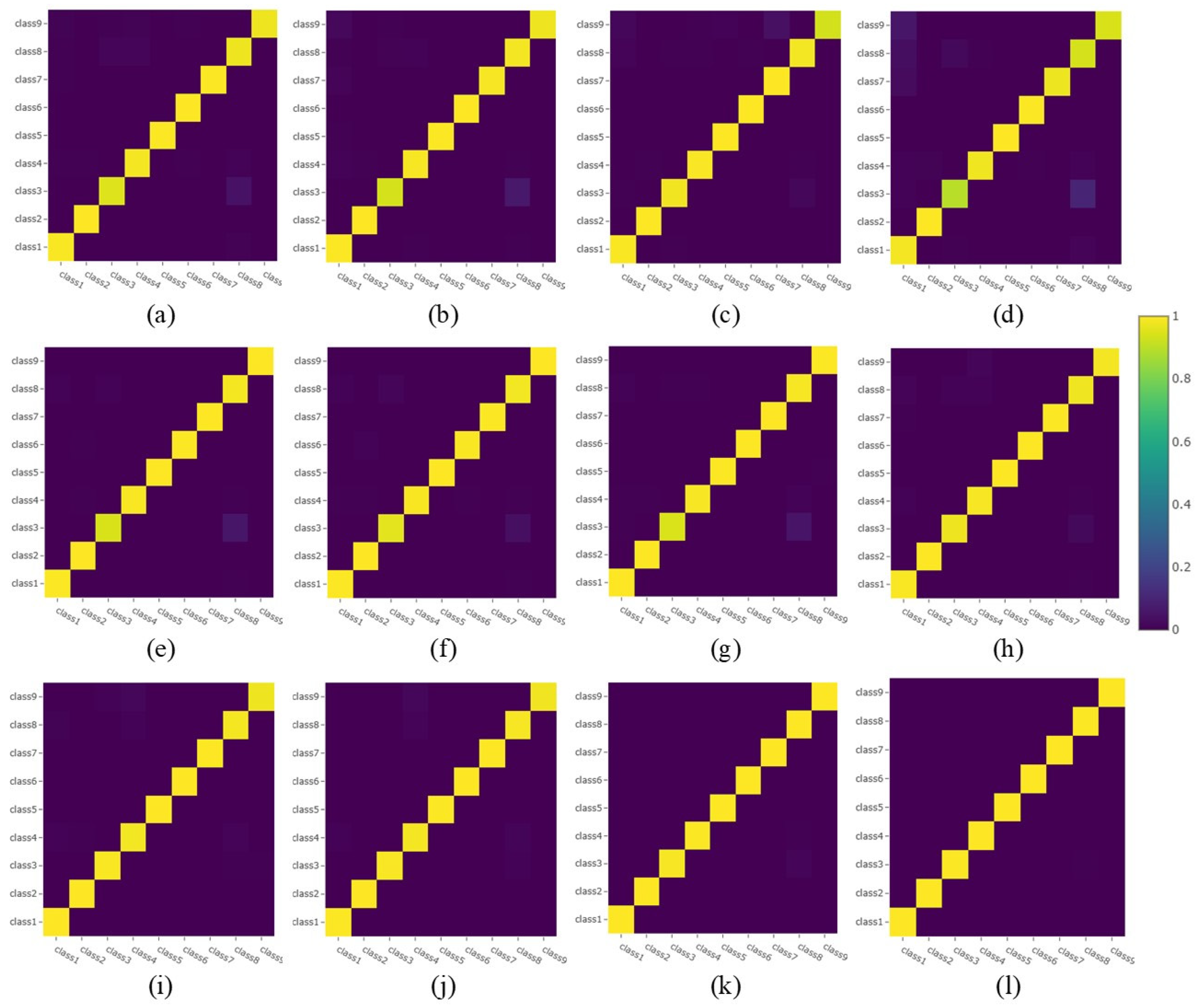
The issue of class imbalance poses a challenge for HSI classification. For example, the seventh class (grass—pasture-mowed) and the ninth class (oats) in the IP dataset, as well as the fifth (painted metal sheets), seventh (bitumen), and ninth (shadows) classes in the PU dataset.

Observing Table 4, SSFTT (36.11% ± 14.96), MSNAT (48.89% ± 19.85), and other well-performing methods still underperform for the accuracy of the ninth class in the IP dataset. Similarly, DeepViT is only 64.40% ± 12.58, and SSFTT is 78.40% ± 28.41 for the accuracy of the seventh class. However, morphFormer achieves relatively better performance in the seventh class (100.00% ± 0.00) and the ninth class (70.56% ± 16.11), likely due to the introduction of mathematical morphology into the model, which enables it to learn more intrinsic shape information. It is worth noting that our MDFFN obtains the best classification results on the seventh (100.00% ± 0.00) and ninth (87.78% ± 4.16) classes, improving 21.6% and 51.67% compared to SSFTT, and 5.6% and 38.89% compared to MSNAT, respectively. In terms of overall performance, the AA of MDFFN is 98.05% ± 0.32, which increases by 1.55% compared to the second-best performing model, morphFormer. Precisely because our method enables effective fine multi-scale feature extraction, which better addresses the classification of small target samples. In addition, on the PU dataset (see Table 5), MDFFN reaches 100% optimal accuracy in the fifth, seventh, and ninth classes. The above results confirm that our approach could comprehensively extract discriminative features from HSI, enabling the network to achieve satisfactory performance even with imbalanced data, thus ensuring an overall improvement in accuracy.

4.

The visualization of confusion matrices on imbalanced datasets

To further visualize the contributions of various methods for different classes in imbalanced datasets, Figure 4 and Figure 5 present the confusion matrix visualizations for different methods on the IP and PU datasets. Due to the significant disparities in sample numbers between the classes in these imbalanced datasets, we normalize the confusion matrices to more clearly evaluate the classification performance. Observing Figure 4 and Figure 5, we find that the main diagonal of MDFFN’s confusion matrix is brighter and more consistent compared to other methods, indicating that our approach achieves satisfactory performance across classes, particularly in minority classes. For minority classes, Table 4 shows that the color blocks for the seventh and ninth classes in MDFFN are more concentrated than others, signifying fewer misclassifications. Similarly, Table 5 reveals that the color for the ninth class in MDFFN is brighter than that in HybridSN, M3D-DCNN, and SSFTT, suggesting higher accuracy. Additionally, in other classes, such as the 1st and 16th classes in the IP dataset and the 3rd class in the PU dataset, our method also outperforms others. This indicates that the proposed MDFFN not only improves the accuracy of small-sample classes but also ensures the stability of other classes, verifying its superiority in processing imbalanced datasets.

4.3.2. Visual Evaluation

To visually demonstrate the classification results, Figure 6, Figure 7 and Figure 8 present the performance in the form of classification maps of all compared methods on the IP, PU, and Houston 2013 datasets. From visual classification maps, the results indicate that MDFFN achieves the maps closest to the ground truth, with fewer misclassified pixels and cleaner boundaries, delivering the best classification performance.

Specifically, for the IP dataset, where the pixels of the same class are relatively concentrated, our method obtains the results closest to the ground truth compared to other methods. As shown in Figure 6, the “Soybean—clean” class contains more noise and is frequently misclassified as the “Corn—no till” class, especially in CNN-based methods (See Figure 6c–f). In contrast, MDFFN shows the most consistent color distribution. The PU and Houston 2013 datasets have more isolated pixels and small regions, which could pose a challenge for the classifier. Remarkably, MDFFN maintains the best overall consistency in various regions compared to other models. This advantage is particularly evident in critical regions like “Self-blocking bricks” in PU and “Parking lot 2” in Houston 2013. The visual comparisons further highlight the effectiveness of the proposed MDFFN. Our methodology combines the multi-scale feature extraction capability of the MCIE module with the cross-scale deep fusion mechanism of the DACA module. This design demonstrates the significant advantages of the MDFFN in fine feature extraction and deep feature fusion, enabling effective characterization of land-cover types with varying spatial shapes and sizes, thereby improving classification accuracy.

However, Figure 6 also reveals that MDFFN still exhibits some misclassifications between adjacent pixels in small regions, such as at the boundary between the “Soybean—min till” and “Corn—no till” classes in the IP dataset. Although our method achieves a clearer division in this region compared to others, there remains room for improvement. This may be due to the similar spectral–spatial features between different classes in the transitional zone of the small regions. Future work could explore strategies such as morphological operations for boundary prior constraints to enhance the ability of the model to detect subtle boundaries, thereby further improving its discriminative performance in complex scenarios.

4.3.3. Efficiency Analysis

To comprehensively evaluate the efficiency of different methods in hyperspectral image classification,

Table 7. Comparison results of efficiency on the IP dataset.

Methods	Params (MB)	FLOPs (GB)	Training Time (s)	Testing Time (s)
2D-CNN	0.39	0.02	10.04	0.62
3D-CNN	0.26	0.04	17.36	0.90
HybridSN	1.19	0.11	14.46	0.88
M3D-DCNN	0.21	0.03	16.17	0.78
ViT	9.60	0.50	27.59	1.19
CrossViT	69.87	2.29	93.68	4.07
DeepViT	9.60	0.50	34.04	1.34
SpectralFormer	0.14	0.01	114.71	16.17
SSFTT	0.15	0.03	12.80	0.76
morphFormer	0.06	0.01	52.57	2.63
MSNAT	0.12	0.02	35.75	0.99
MDFFN	21.15	0.78	57.15	1.93

lists the number of parameters, the floating point operations (FLOPs), the training time, and the testing time of each method on the IP datasets. From the results, the proposed MDFFN exhibits higher parameters and FLOPs compared to other methods, and its speed efficiency is less than satisfactory, which represents a limitation of our approach. This is due to the complexity of the MDFFN model design based on the improved multi-scale CrossViT. In this design, the transformer requires multiple stacks of self-attention modules to learn features, affecting the model’s efficiency. However, previous comparative experiments and visual evaluations have validated the superiority of MDFFN in classification performance (see Section 4.3.1 and Section 4.3.2). The outstanding classification performance of our approach combined with its effective handling of imbalanced data compensates for the weakness of efficiency. Overall, we consider the balance between performance and efficiency in MDFFN acceptable. In addition, as shown in Table 7, the parameters and FLOPs of MDFFN are improved by nearly three times compared with its counterpart CrossViT. The training time is lower than CrossViT and SpectralFormer, and close to morphFormer. This further demonstrates that MDFFN could achieve excellent classification performance at an appropriate computational cost, offering a feasible solution for HSI classification tasks.

4.3.4. Ablation Experiments

We further conduct ablation experiments on the three datasets to explore the effect of the MCIE and DACA modules in the proposed MDFFN. The experimental configurations are as follows:

(a)

The CrossViT model with multi-scale feature fusion is selected as the basic architecture.

(b)

To validate the effectiveness of the multi-scale convolutional information embedding module in MDFFN, the experiment uses the linear projection embedding module based on CrossViT as a comparison.

(c)

To validate the effectiveness of the dual aggregation cross-attention module in MDFFN, the experiment adopts the cross-attention module based on CrossViT as a comparison.

• The performance for different combinations of the modules

We evaluated the performance of the modules by considering four different combinations with quantitative comparisons tabulated in

Table 8. Ablation experiments of the MCIE and DACA module in MDFFN on IP, PU, and Houston 2013 datasets.

Case	Dataset	Module		OA (%)	AA (%)	Kappa (%)
		MCIE	DACA
1	Indian Pines	×	×	90.49 ± 0.69	88.39 ± 1.06	89.12 ± 0.79
2		×	√	94.07 ± 0.26	91.70 ± 0.75	93.22 ± 0.29
3		√	×	97.52 ± 0.35	95.44 ± 0.97	97.17 ± 0.40
4		√	√	98.85 ± 0.09	98.05 ± 0.32	98.69 ± 0.10
1	Pavia University	×	×	98.57 ± 0.12	97.85 ± 0.23	98.10 ± 0.16
2		×	√	99.14 ± 0.09	98.72 ± 0.10	98.86 ± 0.12
3		√	×	99.89 ± 0.03	99.82 ± 0.06	99.86 ± 0.04
4		√	√	99.96 ± 0.02	99.93 ± 0.04	99.95 ± 0.02
1	Houston 2013	×	×	96.37 ± 0.29	95.69 ± 0.39	96.07 ± 0.31
2		×	√	97.96 ± 0.10	97.43 ± 0.12	97.79 ± 0.11
3		√	×	98.90 ± 0.15	99.07 ± 0.14	98.81 ± 0.16
4		√	√	99.42 ± 0.07	99.49 ± 0.07	99.37 ± 0.08

The bold entities indicate the highest value. ×: does not exist, √: exists.

. Case 1 represents the configuration without the MCIE and DACA modules, Case 2 uses the DACA module, Case 3 uses the MCIE module, and Case 4 incorporates both the MCIE and DACA modules. To further explore the contributions of each module, Figure 9 shows the classification accuracy of classes for different cases on the imbalanced dataset.

The contribution of the MCIE module significantly improves the classification performance of the network, as demonstrated by the results of Case 1 and Case 3 in Table 8. Specifically, on the IP, PU, and Houston 2013 datasets, the OA increased by 7.03%, 1.32%, and 2.53%, respectively, while the AA improved by 7.05%, 1.97%, and 3.38%. Furthermore, the Kappa shows an enhancement of 8.05%, 1.76%, and 2.74%. These results indicate that the MCIE module can adequately capture important spatial–spectral features at different scales to highlight discriminative information for improved classification accuracy. Additionally, Figure 9 shows that for small sample classes such as the seventh and ninth classes, Case 3 achieves the fastest improvement in accuracy. For classes with a relatively ample number of samples, such as the 2nd and 12th classes, Case 3 also exhibits significant improvement. This validates the superiority of the MCIE module in handling imbalanced samples, as it can preserve more effective spatial and spectral information, enabling the extraction of key features even in classes with fewer samples.

Similarly, the contribution of the DACA module is reflected in the improvement in classification performance on different datasets. As shown in Case 1 and Case 2 in Table 8, the OA is improved by 3.58%, 0.57%, and 1.59%, AA by 3.31%, 0.87%, and 1.74%, and the Kappa by 4.10%, 0.76%, and 1.72% on the IP, PU, and Houston 2013 datasets, respectively, which validates the DACA module is more effective in achieving deep feature perception compared to employing cross-attention. This may be because cross-attention leads to the weakening of some important features that are weakly autocorrelated in the single branch but significant in cross-scale information. In contrast, our method effectively mitigates the above issue by employing a cross-scale interaction strategy and a dual aggregation mechanism. Additionally, as shown in Figure 9, Case 2 achieves significant improvements in classes such as the 7th and 15th classes. This proves the effectiveness of the DACA module, highlighting its ability to fully facilitate deep fusion between multi-scale features and providing a strong feature representation capability.

According to Table 8, it can be observed that the combination of two modules (Case 4) achieves the highest OA, AA, and Kappa on all datasets, with the OA of 98.85% ± 0.09, 99.96% ± 0.02, and 99.42% ± 0.07. Figure 9 also clearly demonstrates that Case 4 achieves the highest accuracy across all classes, which further validates the superiority of the proposed MDFFN. This is precisely because our method fully leverages the rich spatial–spectral information in HSI, enabling a more comprehensive extraction of local and global features. By employing the MCIE module to effectively extract multi-scale fine features, and combining it with the DACA module to enhance the synergy between different features, the shallow feature extraction from the MCIE module is elevated to deep feature fusion, resulting in superior performance.

2.

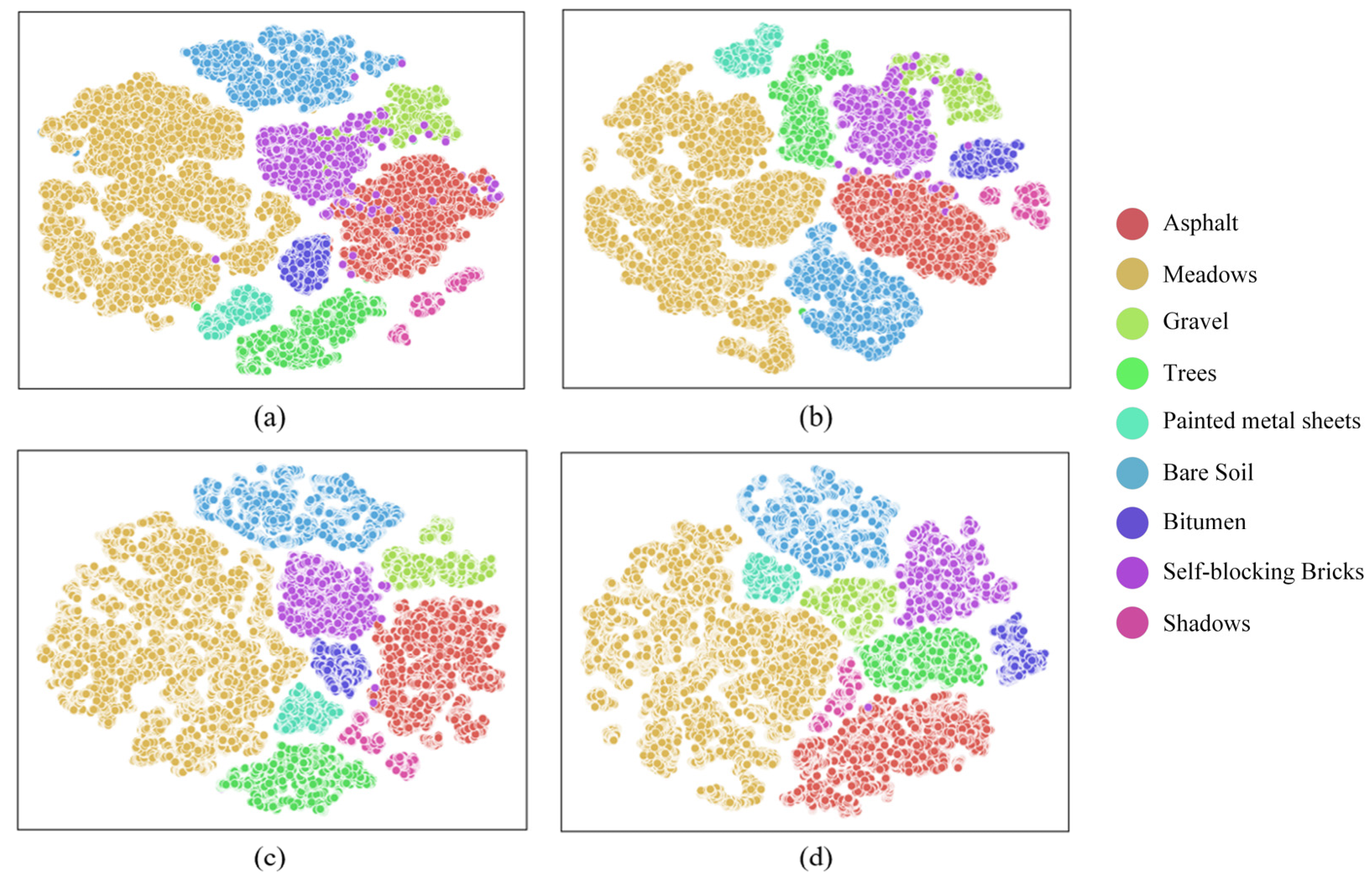
The visualization of feature maps of each module

To further demonstrate the feature extraction capabilities of each module, we use t-distributed stochastic neighbor embedding (T-SNE) [47] to visualize the feature separability extracted from the PU dataset for different cases, as shown in Figure 10. From Figure 10, it can be found that feature clustering is achieved for all four cases. Specifically, Case 1 has an obvious overlap between different classes, and the points of the same class are more scattered, failing to form a good clustering effect. Comparing Case 1 and Case 3, Case 3 can clearly separate the classes, with almost no mixing between the “Trees” and “Self-blocking bricks” classes, which proves the superior feature extraction ability of the MCIE module. Furthermore, comparing Case 3 and Case 4, the feature clusters in Case 4 are more complete and compact. It better separates the “Asphalt” and “Self-blocking bricks” classes, and the distributions for the “Trees” and “Shadows” classes are more uniform. This indicates that incorporating the DACA module further enhances the features, making it easier for the network to extract features conducive to classification and reducing interference by neighboring classes.

4.3.5. Parameter Sensitivity Experiments

To assess the performance of the model comprehensively, we conduct experiments to investigate the parameter sensitivity of the proposed MDFFN for analyzing the effects of different parameter settings on HSI classification, including various combinations of S-branch size and L-branch size, different depths of the multi-scale transformer, and different proportions of training samples. The detailed results are presented in

Table 9. The performance of the MDFFN with different sizes of S-branch size and L-branch on the IP dataset.

Spatial Size	S-Branch (${\mathit{P}}_{\mathbf{S}}$)	L-Branch (${\mathit{P}}_{\mathbf{L}}$)	OA (%)	AA (%)	Kappa (%)	FLOPs (G)	Params (M)
10	2	5	98.02 ± 0.16	95.87 ± 0.74	97.74 ± 0.18	0.66	20.92
12	2	6	98.51 ± 0.10	96.08 ± 0.95	98.29 ± 0.12	0.90	21.03
15	3	5	98.85 ± 0.09	98.05 ± 0.32	98.69 ± 0.10	0.78	21.15
18	3	6	99.04 ± 0.12	98.22 ± 0.73	98.90 ± 0.14	1.05	21.39
20	4	5	98.96 ± 0.12	98.34 ± 0.42	98.81 ± 0.13	0.96	21.51
24	4	6	98.80 ± 0.04	97.71 ± 0.53	98.63 ± 0.05	1.27	21.96

The bold entities indicate the highest value.

and

Table 10. The performance of the MDFFN with different depths of multi-scale transformer on the IP dataset.

Depth	OA (%)	AA (%)	Kappa (%)	FLOPs (G)	Params (M)
1	98.28 ± 0.15	97.05 ± 0.44	98.04 ± 0.17	0.28	7.23
3	98.85 ± 0.09	98.05 ± 0.32	98.69 ± 0.10	0.78	21.15
5	98.91 ± 0.04	98.34 ± 0.58	98.76 ± 0.05	1.28	35.07
7	98.85 ± 0.06	97.40 ± 0.45	98.68 ± 0.07	1.78	48.98
9	98.84 ± 0.11	97.58 ± 0.92	98.68 ± 0.13	2.28	62.90

The bold entities indicate the highest value.

and Figure 11 and Figure 12.

• Combinations in multi-scale patch sizes

The different scale sizes would affect the classification performance of the model. Table 9 shows the classification results of the MDFFNB with different scale combinations on the IP dataset. In the experiment, we set the spatial sizes to 10, 12, 15, 18, 20, and 24, selecting 2, 3, and 4 as the patch sizes for S-branch as well as 5 and 6 for L-Branch. In Table 9, the results reveal that the OA, AA, and Kappa exhibit a trend of first increasing and then decreasing as the spatial size increases, where the best values are 99.04% ± 0.12, 98.34% ± 0.42, and 98.90% ± 0.14. The reason is that although the larger image blocks provide more spatial information, they lead to more complexity in extracting the spatial–spectral features. We could also find that as the patch size increases, both the params and FLOPs increase, consuming more resources and potentially affecting the performance of the model (e.g., combinations of (4, 5) and (4, 6)). Moreover, we can intuitively observe that the combination of (3, 6) for the S-branch and L-branch achieves the best performance. The combination not only allows the extraction of more diverse and richer features but also avoids excessive repetitive and redundant information. Therefore, we can comprehensively consider both model performance and efficiency, selecting the appropriate combination according to the specific application scenario to achieve an optimal balance. For real-time processing tasks, we should prioritize combinations with higher computational efficiency. Conversely, for tasks requiring high accuracy, a higher computational cost can be accepted to obtain better performance, such as the combination of (3, 6).

2.

Number of multi-scale transformer layers

Depth is defined as the number of multi-scale transformer layers applied. We investigate the impact of different depths of the multi-scale transformer in MDFFN on the classification results. Generally, increasing the depth can capture more complex features and long-range dependencies, but an excessively deep architecture may lead to the attenuation of dependency information and increase the computational burden. In the experiment, we set the depth to 1, 3, 5, 7, and 9. According to Table 10, in the IP dataset, as the number of layers increases from 1 to 5, the classification performance is improved due to the greater feature extraction capability of the model and the increase in the number of learnable parameters. Specifically, the OA is improved by 0.63% from 98.28% ± 0.15 to 98.91% ± 0.04. However, continuously increasing the number of stacks does not lead to an additional performance boost. When the number of layers is increased from 5 to 9, the classification performance declines. This could be due to the small proportion of training samples. The use of multiple transformer layers introduces a large number of redundant parameters, increasing the complexity of the model. This leads to overfitting and ultimately impacts performance.

3.

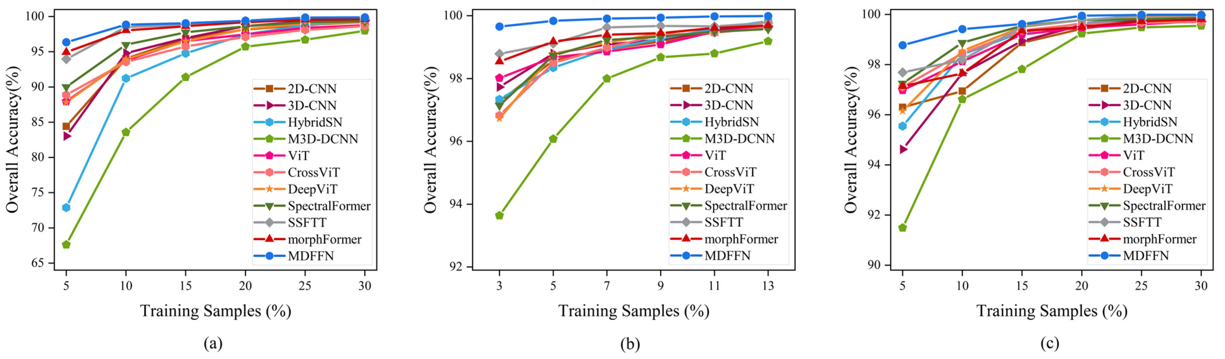
Proportion of training samples

To assess the generalization ability of the model, we conduct experiments with varying proportions of training samples. Taking into account the sample size of each dataset and the performance in previous experiments, we set the training sample ratio for the IP and Houston 2013 datasets, which have relatively fewer samples, to range from 5% to 30% (with a 5% interval). For the PU dataset, the ratio is set from 3% to 13% (with a 2% interval). This could more comprehensively reflect the impact of training data variations on model performance. As shown in Figure 11, MDFFN achieves the highest OA of 96.36% and 98.78% at the 5% training sample ratio for the IP and Houston 2013 datasets, respectively. For the PU dataset, the highest OA of 99.66% is achieved at the 3% training sample ratio. These results demonstrate that our approach performs best with small samples, compared to the others. As the proportion of training samples increases, the performance of each method gradually improves and tends to stabilize. Among them, MDFFN shows a more stable trend across different datasets. For example, in the 3–5% range of the PU dataset, MDFFN increased by only 0.18%, while M3D-DCNN increased by 2.44% and CrossViT by 1.67%, which proves the model’s excellent stability. Compared to other methods, MDFFN consistently outperforms the others across different training sample ratios, confirming that the proposed MDFFN has superior classification performance and generalization ability.

In addition, to further explore the performance of the proposed MDFFN in an imbalanced environment, we adjust the training sample ratio to 5% and choose different types of methods for comparison, including 3D-CNN, CrossViT, and morphFormer. These methods outperformed the other same type methods in the minority classes of the previous experiments (with a 10% training sample ratio). According to Figure 12, the proposed MDFFN still performs best in minority classes, particularly in the seventh class, where its accuracy is significantly higher than that of 3D-CNN and CrossViT. This further validates the robust generalization capability of MDFFN on imbalanced data.

5. Conclusions

In this paper, in order to effectively achieve fine feature extraction and deep feature fusion for HSI, we propose the multi-scale dual-aggregated feature fusion network for HSI classification. Under the multi-scale framework, the MDFFN method combines the advantages of CNN in local feature extraction and transformer in global feature extraction, resulting in outstanding classification performance. In particular, we design the MCIE module, which employs a multi-scale pooling operation to aggregate local features, highlighting discriminative information. We also propose the DACA module, which uses a cross-scale interaction strategy to ensure the deep fusion of different features and adopts a dual aggregation mechanism to mitigate the information loss, further enhancing the spatial–spectral features and providing high-level semantic information for the entire architecture. Extensive experiments conducted on the three HSI datasets demonstrate that the proposed MDFFN achieves more competitive classification performance compared to other state-of-the-art methods, and even could learn critical features from small target samples, effectively reducing misclassification in imbalanced datasets. These results highlight the strong feature representation capability and superior generalization performance of the proposed method.

Building upon this research, we could attempt two aspects of work. The first involves exploring more lightweight and efficient architectures that further reduce the model complexity while maintaining the classification performance, thereby improving the model’s applicability in complex real-world scenarios. The second focuses on integrating multimodal data to improve classification accuracy and robustness, thus providing technical support for realizing more reliable classification tasks.

References

1. Khan, A.; Vibhute, A.D.; Mali, S.; Patil, C.H. A Systematic Review on Hyperspectral Imaging Technology with a Machine and Deep Learning Methodology for Agricultural Applications. Ecol. Inform. 2022, 69, 101678. [Google Scholar] [CrossRef]
2. Alboody, A.; Vandenbroucke, N.; Porebski, A.; Sawan, R.; Viudes, F.; Doyen, P.; Amara, R. A New Remote Hyperspectral Imaging System Embedded on an Unmanned Aquatic Drone for the Detection and Identification of Floating Plastic Litter Using Machine Learning. Remote Sens. 2023, 15, 3455. [Google Scholar] [CrossRef]
3. Sousa, F.J.; Sousa, D.J. Hyperspectral Reconnaissance: Joint Characterization of the Spectral Mixture Residual Delineates Geologic Unit Boundaries in the White Mountains, CA. Remote Sens. 2022, 14, 4914. [Google Scholar] [CrossRef]
4. Zhu, W.; Sun, X.; Zhang, Q. DCG-Net: Enhanced Hyperspectral Image Classification with Dual-Branch Convolutional Neural Network and Graph Convolutional Neural Network Integration. Electronics 2024, 13, 3271. [Google Scholar] [CrossRef]
5. Rao, W.; Gao, L.; Qu, Y.; Sun, X.; Zhang, B.; Chanussot, J. Siamese Transformer Network for Hyperspectral Image Target Detection. IEEE Trans. Geosci. Remote Sens. 2022, 60, 5526419. [Google Scholar] [CrossRef]
6. Zhang, H.; Liu, H.; Yang, R.; Wang, W.; Luo, Q.; Tu, C. Hyperspectral Image Classification Based on Double-Branch Multi-Scale Dual-Attention Network. Remote Sens. 2024, 16, 2051. [Google Scholar] [CrossRef]
7. Liu, G.; Wang, L.; Liu, D.; Fei, L.; Yang, J. Hyperspectral Image Classification Based on Non-Parallel Support Vector Machine. Remote Sens. 2022, 14, 2447. [Google Scholar] [CrossRef]
8. Yuan, S.; Sun, Y.; He, W.; Gu, Q.; Xu, S.; Mao, Z.; Tu, S. MSLM-RF: A Spatial Feature Enhanced Random Forest for On-Board Hyperspectral Image Classification. IEEE Trans. Geosci. Remote Sens. 2022, 60, 5534717. [Google Scholar] [CrossRef]
9. Wang, X. Hyperspectral Image Classification Powered by Khatri-Rao Decomposition-Based Multinomial Logistic Regression. IEEE Trans. Geosci. Remote Sens. 2022, 60, 5530015. [Google Scholar] [CrossRef]
10. Lv, N.; Han, Z.; Chen, C.; Feng, Y.; Su, T.; Goudos, S.; Wan, S. Encoding Spectral-Spatial Features for Hyperspectral Image Classification in the Satellite Internet of Things System. Remote Sens. 2021, 13, 3561. [Google Scholar] [CrossRef]
11. Chen, C.; Ma, Y.; Ren, G. Hyperspectral Classification Using Deep Belief Networks Based on Conjugate Gradient Update and Pixel-Centric Spectral Block Features. IEEE J. Sel. Top. Appl. Earth Obs. Remote Sens. 2020, 13, 4060–4069. [Google Scholar] [CrossRef]
12. Yu, C.; Han, R.; Song, M.; Liu, C.; Chang, C.-I. Feedback Attention-Based Dense CNN for Hyperspectral Image Classification. IEEE Trans. Geosci. Remote Sens. 2022, 60, 5501916. [Google Scholar] [CrossRef]
13. Mei, S.; Li, X.; Liu, X.; Cai, H.; Du, Q. Hyperspectral Image Classification Using Attention-Based Bidirectional Long Short-Term Memory Network. IEEE Trans. Geosci. Remote Sens. 2022, 60, 5509612. [Google Scholar] [CrossRef]
14. Wang, J.; Guo, S.; Huang, R.; Li, L.; Zhang, X.; Jiao, L. Dual-Channel Capsule Generation Adversarial Network for Hyperspectral Image Classification. IEEE Trans. Geosci. Remote Sens. 2022, 60, 5501016. [Google Scholar] [CrossRef]
15. Ye, Z.; Li, C.; Liu, Q.; Bai, L.; Fowler, J. Computationally Lightweight Hyperspectral Image Classification Using a Multiscale Depthwise Convolutional Network with Channel Attention. IEEE Geosci. Remote Sens. Lett. 2023, 20, 1–5. [Google Scholar] [CrossRef]
16. Dosovitskiy, A.; Beyer, L.; Kolesnikov, A.; Weissenborn, D.; Zhai, X.; Unterthiner, T.; Dehghani, M.; Minderer, M.; Heigold, G.; Gelly, S.; et al. An Image Is Worth 16x16 Words: Transformers for Image Recognition at Scale. arXiv 2021, arXiv:2010.11929v2. [Google Scholar]
17. Zhou, D.; Kang, B.; Jin, X.; Yang, L.; Lian, X.; Jiang, Z.; Hou, Q.; Feng, J. DeepViT: Towards Deeper Vision Transformer. arXiv 2021, arXiv:2103.11886. [Google Scholar]
18. Chen, C.-F.; Fan, Q.; Panda, R. CrossViT: Cross-Attention Multi-Scale Vision Transformer for Image Classification. 2021. Available online: https://openaccess.thecvf.com/content/ICCV2021/papers/Chen_CrossViT_Cross-Attention_Multi-Scale_Vision_Transformer_for_Image_Classification_ICCV_2021_paper.pdf (accessed on 7 September 2024).
19. Sun, L.; Zhao, G.; Zheng, Y.; Wu, Z. Spectral–Spatial Feature Tokenization Transformer for Hyperspectral Image Classification. IEEE Trans. Geosci. Remote Sens. 2022, 60, 5522214. [Google Scholar] [CrossRef]
20. Roy, S.K.; Deria, A.; Shah, C.; Haut, J.M.; Du, Q.; Plaza, A. Spectral–Spatial Morphological Attention Transformer for Hyperspectral Image Classification. IEEE Trans. Geosci. Remote Sens. 2023, 61, 5503615. [Google Scholar] [CrossRef]
21. Shu, Z.; Wang, Y.; Yu, Z. Dual Attention Transformer Network for Hyperspectral Image Classification. Eng. Appl. Artif. Intell. 2024, 127, 107351. [Google Scholar] [CrossRef]
22. Qiao, X.; Roy, S.K.; Huang, W. Multiscale Neighborhood Attention Transformer with Optimized Spatial Pattern for Hyperspectral Image Classification. IEEE Trans. Geosci. Remote Sens. 2023, 61, 5523815. [Google Scholar] [CrossRef]
23. Wang, X.; Sun, L.; Lu, C.; Li, B. A Novel Transformer Network with a CNN-Enhanced Cross-Attention Mechanism for Hyperspectral Image Classification. Remote Sens. 2024, 16, 1180. [Google Scholar] [CrossRef]
24. Wang, W.; Liu, L.; Zhang, T.; Shen, J.; Wang, J.; Li, J. Hyper-ES2T: Efficient Spatial–Spectral Transformer for the Classification of Hyperspectral Remote Sensing Images. Int. J. Appl. Earth Obs. Geoinf. 2022, 113, 103005. [Google Scholar] [CrossRef]
25. Gong, H.; Li, Q.; Li, C.; Dai, H.; He, Z.; Wang, W.; Li, H.; Han, F.; Tuniyazi, A.; Mu, T. Multiscale Information Fusion for Hyperspectral Image Classification Based on Hybrid 2D-3D CNN. Remote Sens. 2021, 13, 2268. [Google Scholar] [CrossRef]
26. Wang, A.; Zhang, K.; Wu, H.; Iwahori, Y.; Chen, H. Multi-Scale Residual Spectral–Spatial Attention Combined with Improved Transformer for Hyperspectral Image Classification. Electronics 2024, 13, 1061. [Google Scholar] [CrossRef]
27. Hu, W.; Huang, Y.; Wei, L.; Zhang, F.; Li, H. Deep Convolutional Neural Networks for Hyperspectral Image Classification. J. Sens. 2015, 2015, 258619. [Google Scholar] [CrossRef]
28. Hamouda, M.; Ettabaa, K.S.; Bouhlel, M.S. Smart Feature Extraction and Classification of Hyperspectral Images Based on Convolutional Neural Networks. IET Image Process. 2020, 14, 1999–2005. [Google Scholar] [CrossRef]
29. Fei, X.; Wu, S.; Miao, J.; Wang, G.; Sun, L. Lightweight-VGG: A Fast Deep Learning Architecture Based on Dimensionality Reduction and Nonlinear Enhancement for Hyperspectral Image Classification. Remote Sens. 2024, 16, 259. [Google Scholar] [CrossRef]
30. He, K.; Zhang, X.; Ren, S.; Sun, J. Deep Residual Learning for Image Recognition. In Proceedings of the 2016 IEEE Conference on Computer Vision and Pattern Recognition (CVPR), Las Vegas, NV, USA, 27–30 June 2016; pp. 770–778. [Google Scholar]
31. Hu, T.; Yuan, J.; Wang, X.; Yan, C.; Ju, X. Spectral-Spatial Features Extraction of Hyperspectral Remote Sensing Oil Spill Imagery Based on Convolutional Neural Networks. IEEE Access 2022, 10, 127969–127983. [Google Scholar] [CrossRef]
32. Zhang, X.; Guo, Y.; Zhang, X. Hyperspectral Image Classification Based on Optimized Convolutional Neural Networks with 3D Stacked Blocks. Earth Sci. Inf. 2022, 15, 383–395. [Google Scholar] [CrossRef]
33. Roy, S.K.; Krishna, G.; Dubey, S.R.; Chaudhuri, B.B. HybridSN: Exploring 3-D–2-D CNN Feature Hierarchy for Hyperspectral Image Classification. IEEE Geosci. Remote Sens. Lett. 2020, 17, 277–281. [Google Scholar] [CrossRef]
34. Hong, D.; Han, Z.; Yao, J.; Gao, L.; Zhang, B.; Plaza, A.; Chanussot, J. SpectralFormer: Rethinking Hyperspectral Image Classification with Transformers. IEEE Trans. Geosci. Remote Sens. 2022, 60, 5518615. [Google Scholar] [CrossRef]
35. Yang, X.; Cao, W.; Lu, Y.; Zhou, Y. Hyperspectral Image Transformer Classification Networks. IEEE Trans. Geosci. Remote Sens. 2022, 60, 5528715. [Google Scholar] [CrossRef]
36. He, M.; Li, B.; Chen, H. Multi-Scale 3D Deep Convolutional Neural Network for Hyperspectral Image Classification. In Proceedings of the 2017 IEEE International Conference on Image Processing (ICIP), Beijing, China, 17–20 September 2017; pp. 3904–3908. [Google Scholar]
37. Xu, Q.; Xiao, Y.; Wang, D.; Luo, B. CSA-MSO3DCNN: Multiscale Octave 3D CNN with Channel and Spatial Attention for Hyperspectral Image Classification. Remote Sens. 2020, 12, 188. [Google Scholar] [CrossRef]
38. Chen, Y.; Wang, X.; Zhang, J.; Shang, X.; Hu, Y.; Zhang, S.; Wang, J. A New Dual-Branch Embedded Multivariate Attention Network for Hyperspectral Remote Sensing Classification. Remote Sens. 2024, 16, 2029. [Google Scholar] [CrossRef]
39. Li, W.; Chen, H.; Liu, Q.; Liu, H.; Wang, Y.; Gui, G. Attention Mechanism and Depthwise Separable Convolution Aided 3DCNN for Hyperspectral Remote Sensing Image Classification. Remote Sens. 2022, 14, 2215. [Google Scholar] [CrossRef]
40. Liu, Z.; Lin, Y.; Cao, Y.; Hu, H.; Wei, Y.; Zhang, Z.; Lin, S.; Guo, B. Swin Transformer: Hierarchical Vision Transformer Using Shifted Windows. 2021. Available online: https://openaccess.thecvf.com/content/ICCV2021/papers/Liu_Swin_Transformer_Hierarchical_Vision_Transformer_Using_Shifted_Windows_ICCV_2021_paper.pdf (accessed on 10 September 2024).
41. He, W.; Huang, W.; Liao, S.; Xu, Z.; Yan, J. CSiT: A Multi-Scale Vision Transformer for Hyperspectral Image Classification. IEEE J. Sel. Top. Appl. Earth Obs. Remote Sens. 2022, 15, 9266–9277. [Google Scholar] [CrossRef]
42. Chen, H.; Zendehdel, N.; Leu, M.C.; Yin, Z. Fine-Grained Activity Classification in Assembly Based on Multi-Visual Modalities. J. Intell. Manuf. 2024, 35, 2215–2233. [Google Scholar] [CrossRef]
43. Chen, H.; Miao, F.; Chen, Y.; Xiong, Y.; Chen, T. A Hyperspectral Image Classification Method Using Multifeature Vectors and Optimized KELM. IEEE J. Sel. Top. Appl. Earth Obs. Remote Sens. 2021, 14, 2781–2795. [Google Scholar] [CrossRef]
44. Ma, Y.; Wang, S.; Du, W.; Cheng, X. An Improved 3D-2D Convolutional Neural Network Based on Feature Optimization for Hyperspectral Image Classification. IEEE Access 2023, 11, 28263–28279. [Google Scholar] [CrossRef]
45. Gu, Q.; Luan, H.; Huang, K.; Sun, Y. Hyperspectral Image Classification Using Multi-Scale Lightweight Transformer. Electronics 2024, 13, 949. [Google Scholar] [CrossRef]
46. Yang, X.; Ye, Y.; Li, X.; Lau, R.Y.K.; Zhang, X.; Huang, X. Hyperspectral Image Classification with Deep Learning Models. IEEE Trans. Geosci. Remote Sens. 2018, 56, 5408–5423. [Google Scholar] [CrossRef]
47. van der Maaten, L.; Hinton, G. Visualizing Data Using T-SNE. J. Mach. Learn. Res. 2008, 9, 2579–2605. [Google Scholar]
Figure 1. Overview of the MDFFN for HSI classification. MDFFN comprises a multi-scale convolutional information embedding (MCIE) module and a stack of D multi-scale transformer encoders. Each multi-scale transformer encoder employs two different branches (i.e., S-branch and L-branch) to process image tokens of different sizes ( P S and P L , P S < P L ) and uses the dual aggregated cross-attention (DACA) module to achieve efficient fusion. In the figure, * indicates the CLS tokens.
Electronics 14 01477 g001
Figure 2. Multi-scale convolutional information embedding module.
Electronics 14 01477 g002
Figure 3. Dual aggregated cross-attention module for S-branch.
Electronics 14 01477 g003
Figure 4. Visualization of confusion matrices for different methods on the IP dataset: (a) 2D-CNN, (b) 3D-CNN, (c) HybridSN, (d) M3D-DCNN., (e) ViT, (f) CrossViT, (g) DeepViT, (h) SpectralFormer, (i) SSFTT, (j) morphFormer, (k) MSNAT, (l) MDFFN.
Electronics 14 01477 g004
Figure 5. Visualization of confusion matrices for different methods on the PU dataset: (a) 2D-CNN, (b) 3D-CNN, (c) HybridSN, (d) M3D-DCNN, (e) ViT, (f) CrossViT, (g) DeepViT, (h) SpectralFormer, (i) SSFTT, (j) morphFormer, (k) MSNAT, (l) MDFFN.
Electronics 14 01477 g005
Figure 6. Visualizations of classification results on IP dataset. (a) Input image. (b) Ground truth. (c) 2D-CNN. (d) 3D-CNN. (e) HybridSN. (f) M3D-DCNN. (g) ViT. (h) CrossViT. (i) DeepViT. (j) SpectralFormer. (k) SSFTT. (l) morphFormer. (m) MSNAT. (n) MDFFN.
Electronics 14 01477 g006
Figure 7. Visualizations of classification results on PU dataset. (a) Input image. (b) Ground truth. (c) 2D-CNN. (d) 3D-CNN. (e) HybridSN. (f) M3D-DCNN. (g) ViT. (h) CrossViT. (i) DeepViT. (j) SpectralFormer. (k) SSFTT. (l) morphFormer. (m) MSNAT. (n) MDFFN.
Electronics 14 01477 g007
Figure 8. Visualizations of classification results on Houston 2013 dataset. (a) Input image. (b) Ground truth. (c) 2D-CNN. (d) 3D-CNN. (e) HybridSN. (f) M3D-DCNN. (g) ViT. (h) CrossViT. (i) DeepViT. (j) SpectralFormer. (k) SSFTT. (l) morphFormer. (m) MSNAT. (n) MDFFN.
Electronics 14 01477 g008
Figure 9. Classification accuracy of classes for different cases on the IP dataset.
Electronics 14 01477 g009
Figure 10. Visualization of feature separability for different cases on the PU dataset. (a) Case 1. (b) Case 2. (c) Case 3. (d) Case 4.
Electronics 14 01477 g010
Figure 11. The performance of the MDFFN in terms of OA (%) with different training samples on three HSI datasets. (a) Indian Pines. (b) Pavia University. (c) Houston 2013.
Electronics 14 01477 g011
Figure 12. Classification accuracy of minority classes on the IP dataset with a 5% training sample ratio.
Electronics 14 01477 g012