Real-Time Monitoring of LTL Properties in Distributed Stream Processing Applications

Abstract

Stream processing frameworks have become key enablers of real-time data processing in modern distributed systems. However, robust and scalable mechanisms for verifying temporal properties are often lacking in existing systems. To address this gap, a new runtime verification framework is proposed that integrates linear temporal logic (LTL) monitoring into stream processing applications, such as Apache Spark. The approach introduces reusable LTL monitoring patterns designed for seamless integration into existing streaming workflows. Our case study, applied to real-time financial data monitoring, demonstrates that LTL-based monitoring can effectively detect violations of safety and liveness properties while maintaining stable latency. A performance evaluation reveals that although the approach introduces computational overhead, it scales effectively with increasing data volume. The proposed framework extends beyond financial data processing and is applicable to domains such as real-time equipment failure detection, financial fraud monitoring, and industrial IoT analytics. These findings demonstrate the feasibility of real-time LTL monitoring in large-scale stream processing environments while highlighting trade-offs between verification accuracy, scalability, and system overhead.

1. Introduction

Many modern data-driven applications used in healthcare, financial services, e-commerce, and other sectors rely on streams of data to support real-time workflows and quick decision making, where meeting these often very complex operational demands is absolutely imperative [1,2]. However, this efficiency cannot be easily supported when distributed systems create an increasingly massive amount of data that require real-time processing [3,4,5]. Runtime verification (RV) is a lightweight and cost-effective approach recently applied to software systems, with the aim of monitoring their runtime temporal properties in terms of correctness [6,7,8,9]. Among the domains where these issues are crucial, RV has been widely applied in aerospace, automotive safety, and industrial control systems.

Linear temporal logic (LTL) offers an effective method for specifying the temporal properties that systems must maintain, such as safety properties (“something bad never happens”), which can be violated within a finite time frame, and liveness properties (“something good eventually happens”), which can only be violated within an infinite time frame [10,11]. Despite LTL’s strengths, traditional LTL-based RV methods face significant challenges in keeping up with the high-speed, low-latency demands of distributed, large-scale streaming environments. These challenges arise due to the high computational resource demands for monitoring and evaluating temporal properties in real time, necessitating more efficient scalable solutions [8,12]. Despite the suitability of RVs for analyzing temporal properties, they are not designed to function seamlessly with stream processing applications, which prioritize efficient data handling and fault tolerance. This creates a gap in ensuring continuous compliance with system properties during data flow. This study investigates the following key research questions:

• How can LTL-based monitoring be effectively integrated into a distributed streaming application such as Apache Spark to ensure compliance with safety and liveness properties?
• What is the impact of LTL-based monitoring on system performance metrics such as latency and resource utilization?
• How does the system scale with increasing data volume in a distributed stream processing context?

To address these challenges, a new LTL-based RV framework is proposed that integrates real-time monitoring of temporal properties in distributed stream processing. The framework is implemented in Apache Spark, a widely used engine for big data processing [13,14]. However, the proposed approach embeds LTL formulas directly into Spark’s stream processing pipeline, allowing for continuous verification of data streams to ensure compliance with predefined conditions. Specifically, in our case study, we monitor critical financial parameters such as transaction amount, frequency, and amount balance, verifying safety conditions (e.g., “the transaction amount should never exceed a certain threshold”) and liveness conditions (e.g., “the frequency must eventually exceed a critical threshold”). These temporal properties ensure that the system dynamically responds to changing conditions while maintaining operational correctness in real time.

The main contributions of this paper are as follows:

• We present a new approach for integrating LTL-based RV with Apache Spark by embedding LTL formulas into the streaming pipeline for real-time compliance verification, eliminating the need for offline or batch analysis.
• We introduce generalized LTL-based RV patterns for implementing LTL verification in Apache Spark, which can be extended to other stream processing frameworks.
• We propose a scalable and systematic approach for embedding LTL monitoring into stream processing workflows, ensuring low-latency and real-time anomaly detection, while also being adaptable to other stream processing frameworks.
• We validate the effectiveness of our method through a case study on financial data processing and experiments, demonstrating its impact on real-time reliability, correctness, and monitoring of temporal properties such as safety and liveness conditions.

The remainder of this paper is organized as follows: In Section 2 reviews related work on RV and stream processing; Section 3 presents the RV process, focusing on its theoretical foundations and the role of LTL; Section 4 introduces LTL patterns and their integration with Apache Spark for real-time monitoring; Section 5 presents the primary case study, showcasing our approach to real-time monitoring of financial data stream processing, while Section 6 demonstrates its application to real-time monitoring of weather data stream processing; Section 7 outlines the limitations of the current work; Section 8 summarizes the paper, provides conclusions, and outlines future research directions.

2. Related Work

Runtime verification (RV) is used to validate the behavior of a system in real time to ensure that it meets its specifications. Unlike comprehensive functional methods such as model checking and theorem proving, which perform exhaustive verification before deployment, RV is less computationally demanding and suitable for dynamic systems that require real-time verification [6,9]. RV operates alongside the system, monitoring its behavior according to predefined rules and issuing alerts for any anomalies or violations. In particular, RV is suitable for real-time applications that cannot be fully verified prior to use. RV utilizes various logics and specifications, with linear temporal logic (LTL) being the most prominent due to its descriptive power over temporal properties. It has been applied to a wide range of domains, including traditional software systems, embedded systems, and cyber–physical systems, where it is effective in detecting timing errors during runtime. However, conventional RV methods often rely on batch processing techniques used in static analysis, which are not well suited for real-time applications that require low latency and continuous monitoring.

Recent works by Bauer et al. [12] and Leucker [15] provide a comprehensive overview of RV techniques for LTL. Bauer introduces three-valued semantics for LTL and timed LTL, enhancing the applicability of RV to temporal properties where uncertainty is involved. Leucker’s work focuses on applying LTL theorems to RVs, providing a solid theoretical foundation. These studies highlight RV’s ability to capture safety and liveness properties, but do not address the integration with real-time data streaming applications. Maggi et al. [16] applied LTL-based declarative process models to RV, specifically for business processes, indicating that RV is suitable for monitoring compliance in workflows. Similarly, Guang-yuan and Zhi-song [17] introduced linear temporal logic with clocks (LTLC), extending LTL to real-time system verification and demonstrating its effectiveness in ensuring system timeliness. These advancements enhance LTL’s expressiveness but still do not fully meet the demands of high-speed streaming environments. To address the challenges of distributed systems, previous research has focused on failure-aware and decentralized RV techniques. Basin et al. [4] addressed challenges such as network failures and out-of-order message delivery that are typical of distributed systems in the real world. Mostafa and Bonakdarpour [18] further explored these decentralized RV techniques to monitor LTL specifications in distributed systems, demonstrating their applicability through a simulated swarm of flying drones. Similarly, Danielsson and Sánchez [19] proposed decentralized RV techniques for synchronized networks, improving the robustness of RV in environments without synchronized clocks. These approaches have highlighted the potential of RV in decentralized environments, but have not been integrated with modern stream processing frameworks.

Faymonville et al. [20] contributed to the field with their work on parametric temporal logic, which allows dynamic monitoring of systems, particularly in the context of microservices and AI-based systems. This work emphasizes the need for scalability in RV, a key aspect that our proposed approach addresses by integrating with Apache Spark. The field of RV has seen substantial developments in recent years, particularly in addressing the high-speed, low-latency demands of modern stream processing systems. In addition, Zhang and Liu [21] introduced scalable RV solutions for distributed edge computing, emphasizing improved real-time decision making capabilities in environments with limited resources. Similarly, Ganguly et al. [22] addressed the challenges of RV in partially synchronous distributed systems, highlighting issues such as synchronization and fault tolerance. These studies underscore the need for efficient RV frameworks that can operate seamlessly with stream processing systems. Despite these advancements, existing approaches often rely on offline or batch analysis, limiting their utility in real-time applications. The proposed approach is built on these recent advances by integrating LTL-based monitoring directly into Apache Spark. Unlike previous methods that depend on batch processing, we propose a real-time, integrated LTL-based monitoring approach within streaming workflows, as detailed in Section 1. A summary of the related work and how our approach builds on these advances is presented in

Table 1. Comparison of existing works in runtime verification for distributed and real-time systems.

Research Study	Methodology	Benchmark/Metrics	Performance Metrics Evaluated	Strengths	Limitations	How Our Proposed Work Builds Upon Study	Application Domain
Bauer et al. [12]	LTL and TLTL RV with three-valued semantics and minimal deterministic monitors.	Monitor size, early violation detection speed.	Monitor efficiency, detection time.	Reduces ambiguity, optimized monitors.	No real-time streaming integration.	Extends LTL monitoring to distributed streaming (Apache Spark).	General RV.
Leucker [15]	Theoretical LTL-based RV framework.	No specific benchmarks provided.	Not evaluated.	Strong theoretical foundation.	No real-time evaluation.	Implements LTL monitoring in real-time streaming.	Formal verification.
Maggi et al. [16]	Automata-based techniques for RV of LTL-based declarative process models.	No specific benchmarks provided.	Constraint conflict detection, real-time monitoring.	Provides methods for detecting constraint conflicts, uses Declare language and ProM tool set.	Focused on business process monitoring.	Extends automata-based techniques for detecting violations in real-time streams using LTL.	Business processes, constraint-based modeling.
Guang-yuan and Zhi-song [17]	LTLC (Linear Temporal Logic with Clocks) for verifying real-time systems.	No specific benchmarks provided.	Timing precision, overhead analysis.	Improved real-time systems across multiple abstraction levels.	High computational cost in distributed environments.	Adapts real-time constraints for monitoring latency-sensitive stream processing applications.	Real-time systems, embedded systems.
Basin et al. [4]	Online algorithm for RV of distributed systems using MTL.	No specific benchmarks provided.	Handles out-of-order messages, network failures, and supports distributed monitoring.	Supports distributed monitoring with multiple cooperating monitors, robust to failures.	Not optimized for large-scale real-time streaming workloads.	Adapts distributed verification concepts to enhance robustness in streaming LTL monitoring.	Distributed systems, fault-tolerant verification.
Mostafa and Bonakdarpour [18]	Decentralized RV of LTL specifications using distributed computation slicing.	Experimentation on a simulated swarm of drones.	Monitoring overhead, scalability with number of processes.	Fully decentralized approach, linear scalability in monitoring overhead.	No real-time stream processing implementation.	Extends decentralized monitoring techniques to handle large-scale distributed streaming applications.	Swarm robotics, distributed multi-agent systems.
Faymonville et al. [20]	Runtime verification of parametric temporal logic (PLTL).	Complexity analysis of deterministic vs. unambiguous vs. full PLTL.	Space complexity of monitoring algorithms.	Efficient online verification for deterministic/unambiguous PLTL.	High computational cost for full PLTL monitoring.	Extends parametric monitoring concepts to optimize resource-aware LTL monitoring in stream processing.	Parametric verification, real-time system monitoring.
Zhang and Liu [21]	LTLc/CCSL specification language for multi-clock systems.	Model checking for LTLc/CCSL.	Specification of logical clock relations in multi-clock systems.	Formal approach for multi-clock systems, integrates LTLc with CCSL clock calculus.	No direct RV application; focuses on specification.	Integrates logical clock constraints for verifying real-time streaming system schedules.	Multi-clock systems, real-time scheduling.
Ganguly et al. [22]	RV for partially synchronous distributed systems using LTL.	Synthetic case studies and real-world evaluation with Cassandra and NASA RACE data.	Verification efficiency, overhead of monitoring approaches.	Two techniques: automata-based and progression-based formula rewriting; progression-based has lower overhead.	Not optimized for real-time streaming.	Extends partially synchronous runtime verification concepts to improve LTL monitoring in distributed streaming applications.	Distributed databases, aerospace systems (NASA RACE).

.

3. Runtime Verification and Stream Processing Platform

In this section, we provide an overview of runtime verification and its integration into stream processing platforms. In its mathematical essence, RV addresses the word problem, that is, the problem of determining whether a given word (“sequence of events”) belongs to a specific language (“set of desired behaviors”) defined by temporal properties. When combined with stream processing, it facilitates real-time validation of data and system properties, thereby enhancing the reliability of distributed applications. The following subsections cover the fundamentals of RV, its role in software monitoring, and its integration with distributed stream processing platforms for effective real-time verification.

3.1. Runtime Verification

Runtime verification (RV) is a lightweight and dynamic verification technique that is used to monitor software systems during execution [6]. Unlike static analysis, or formal verification [23], which occurs before running time, RV operates in real time, providing immediate feedback on whether a system adheres to predefined properties or requirements. The technique has been a pragmatic way to guarantee reliability in systems when complete formal verification suffers from space explosion [24]. RV achieves this through dynamic observation of system events, running these against specified properties to gain deeper insights into program behavior and conformance with key requirements. The RV process can be visually represented as illustrated in Figure 1.

3.1.1. Preliminaries

In order to understand runtime verification (RV) concepts, we present the following definitions [6]. An event e is an atomic proposition or action observed by the system. Each event has an associated value v, and an observed event instance is denoted as $(e,v)$. A trace $\sigma$ is a finite or infinite sequence of observed events, expressed as $\sigma =e_0,e_1,e_2,\dots$, where $e_i$ represents an event in the sequence, corresponding to a specific state of a system. $ϵ$ represents an empty trace and $\mathrm{Trace}\left(A\right)$ denotes the set of all possible traces over a set of events A. A property $\varphi$ is a formal specification that defines the expected behavior of a system. Given a trace $\sigma$, the notation $\sigma \vDash \varphi$ indicates that $\sigma$ satisfies property $\varphi$. As defined in Equation (1), a monitor M is a state machine that observes execution traces and checks their compliance with a given property $\varphi$.

$$M=\langle Q,\Sigma ,q_0,\delta ,\lambda \rangle$$

(1)

where Q is a finite or infinite set of states. $\sigma$ is the alphabet that represents the set of observed events. $q_0\in Q$ is the initial state. $\delta :Q\times \Sigma \to Q$ is the transition function that maps a pair of state events to a new state. $\lambda :Q\to D$ is the verdict function, where $D=\{\top ,\perp ,?\}$ represents the possible outcomes (true, false, undecided). The verdict function $\lambda$ evaluates whether a trace satisfies the monitored property. An RV system, as defined in Equation (2), is

$$RV=\langle D,A,P,Gen\rangle$$

(2)

where D is the domain of verdicts; A is the set of observed events; P is the set of properties to be monitored; and $Gen$ is a monitor generation function, where $Gen\left(\varphi \right)=M$ maps properties to the monitors.

3.1.2. Linear Temporal Logic (LTL) Syntax and Semantics

LTL extends propositional logic by introducing temporal operators to reason about sequences of states over time. LTL formulas are recursively defined in Equation (3):

$$\varphi ::=\mathrm{true}\mid \mathrm{false}\mid p\mid \neg \varphi \mid {\varphi }_1\wedge {\varphi }_2\mid X\varphi \mid {\varphi }_{1}U{\varphi }_2$$

(3)

where p is an atomic proposition, ¬ and ∧ are standard Boolean operators, X represents the “next” operator, and U is the “until” operator. As defined in Equation (4), the commonly used derived operators F (eventually) and G (globally) are defined as

$$F\varphi \equiv \mathrm{true}U\varphi \mathrm{and}G\varphi \equiv \neg F\neg \varphi .$$

(4)

Given a trace $\sigma =e_0,e_1,e_2,\dots$, the LTL semantics are defined as $\sigma ,i\vDash p$ if the atomic proposition p holds at position i; $\sigma ,i\vDash X\varphi$ if $\varphi$ holds at the next position $i+1$; and $\sigma ,i\vDash {\varphi }_{1}U{\varphi }_2$ if there exists $j\ge i$ such that $\sigma ,j\vDash {\varphi }_2$ and for all $i\le k<j$, $\sigma ,k\vDash {\varphi }_1$. Given a trace $\sigma =e_0,e_1,e_2,\dots$, the semantics of LTL operators are defined as

• $\sigma ,i\vDash p$ if the atomic proposition p holds at position i.
• $\sigma ,i\vDash X\varphi$ if $\varphi$ holds at the next position $i+1$.
• $\sigma ,i\vDash {\varphi }_{1}U{\varphi }_2$ if there exists $j\ge i$ such that $\sigma ,j\vDash {\varphi }_2$ and for all $i\le k<j$, $\sigma ,k\vDash {\varphi }_1$.

3.1.3. Formula and Trace Example

Consider an LTL formula $F{e}_1\wedge G{e}_2$, where $F{e}_1$ (eventually $e_1$) states that there exists a future state where the event $e_1$ holds and $G{e}_2$ (globally $e_2$) states that the event $e_2$ holds in all states of the trace, as shown in Equation (4), for given the trace

$$\sigma =\left\{e_2\right\},\{e_1,e_2\},\left\{e_2\right\},\left\{e_2\right\},\dots$$

(5)

Each set represents a system state where the listed events hold. $e_1$ appears in the second state ${\sigma }_1$, satisfying $F{e}_1$ since at least one occurrence is sufficient. Similarly, $e_2$ holds in all states, satisfying $G{e}_2$, as shown in Figure 2.

3.2. Stream Processing Platforms

The architecture of the proposed system presents a workflow design that illustrates how runtime verification (RV) can be integrated into distributed stream processing platforms [12,25]. This integration enables improved data validation for real-time applications to maintain temporal correctness. Although these principles are applicable to any general stream processing platform, this paper demonstrates the application of this idea using Apache Spark as the underlying framework [13,14]. The general stream processing workflow can be represented as shown in Figure 3.

At the core of the architecture is the RV monitor, which continuously evaluates incoming data streams against predefined linear temporal logic (LTL) properties. These properties encapsulate critical system behaviors, such as maintaining thresholds (e.g., transaction frequency, account balance, wind speed, UV index), or detecting specific temporal sequences of events. Detected violations are immediately logged and reported to enable timely interventions. Apache Spark serves as the backbone of this architecture, providing a low-latency and scalable platform for stream processing [26]. The unique integration of RV enhances Spark’s capabilities by embedding formal verification techniques into its structured streaming operations. This combination ensures not only high-performance data processing, but also compliance with temporal and logical correctness. Supporting components such as Apache Kafka are used for reliable data ingestion [27], while Docker Compose facilitates scalable deployment in distributed environments. However, these components serve as secondary tools and are not the primary focus of this work. Our architecture introduces a new approach that combines distributed stream processing and formal verification techniques, addressing key challenges in real-time data monitoring by ensuring temporal and logical correctness with scalability and performance.

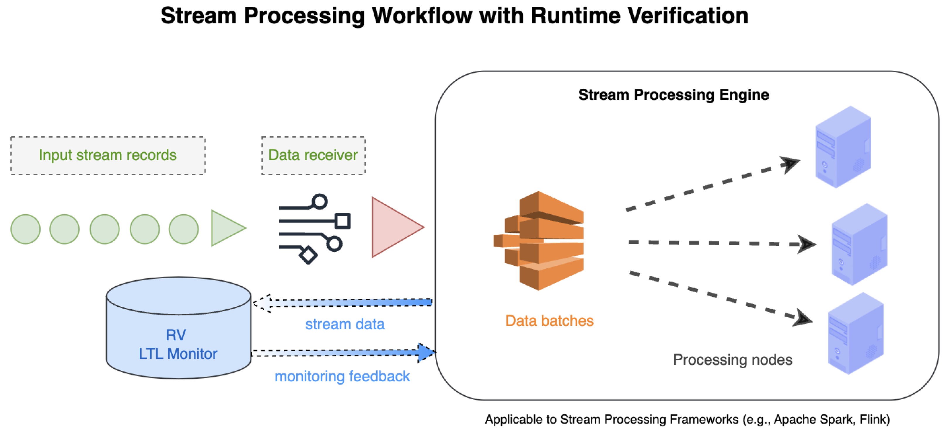
4. LTL-Based RV Patterns in Apache Spark

In this section, reusable patterns are presented for implementing LTL-based RV in Apache Spark’s stream processing. These patterns bridge the gap between LTL semantics and the real-time needs of distributed systems, enabling efficient RV and ensuring system compliance in large-scale applications. As defined in the Preliminaries section, RV relies on state machines that observe execution traces and verify compliance with specified properties. An RV monitor is formally defined in Equation (1), where M transitions between states based on incoming events and produces verdicts indicating whether the monitored system satisfies the given property. In this implementation, LTL operators are mapped to Spark-based monitoring patterns, ensuring efficient real-time verification in a distributed streaming environment.

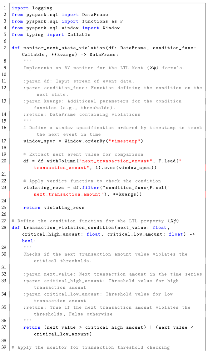
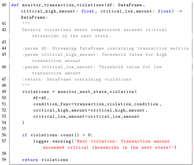
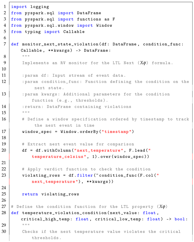
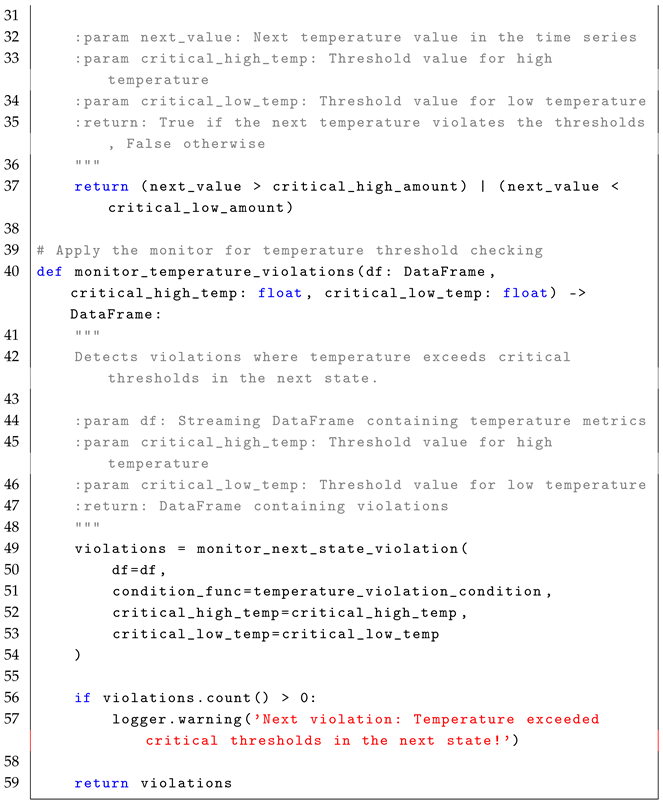
4.1. Next Operator ($X\varphi$)

The formula $X\varphi$ checks whether a given condition $\varphi$ must hold in the next state (immediate next time step). The formal semantics of $X\varphi$ is defined as:

$$\sigma ,i\vDash X\varphi \iff \sigma ,i+1\vDash \varphi$$

(6)

In simple terms, $X\varphi$ means that for a condition $\varphi$ to hold under $X\varphi$, it must be satisfied in the next time step $i+1$. The formula $X\varphi$ is highly relevant in real-time systems where immediate state transitions need to be monitored, such as detecting if performance metrics exceed thresholds in the next event. In real-time stream processing, the formula $X\varphi$ enables the detection of conditions that must hold in the next state in the event stream, as described in the reference monitor approach Algorithm 1

The monitoring process for the $X\varphi$ formula follows a stateless interpretation, where each event in the stream is treated independently to check whether the condition holds in the next event. Conceptually, the set of states, Q, is represented by the rows in the EventStream, with each row corresponding to a potential state at a specific timestamp. The initial state, $q_0$, is implicitly the first row of the DataFrame, ordered by timestamp. The trace, $\sigma$, is defined by the sequence of events or rows in the DataFrame that are observed in the system over time, with each event in the stream representing a state at a particular time stamp. The alphabet of observed events, $\sigma$, refers to structured streaming events such as sensor readings, metrics, or other data points observed in the system. This alphabet represents the set of all possible events that could occur in the stream. The transition function, $\delta$, defines the transition between states over time, tracked by the “lead” function, which retrieves the value of the next event in the time series. The verdict function, $\lambda$, filters events where the condition $X\varphi$ does not hold by checking the current and next events and determining whether the violation condition is met.

The following pseudocode (i.e., Algorithm 1) illustrates the core concept behind monitoring violations of the $X\varphi$ condition in a stream of events.

Algorithm 1 Next State Violation Monitoring for LTL Formula $X\varphi$

1: Input: EventStream (DataFrame), ${\mathrm{ConditionFunction}}_{\varphi }$, AdditionalParameters 2: Output: Violations (DataFrame) 3: Define a window ordered by timestamp to track the next event in time 4: Extract next event value: next_event = lead(event_value, 1) over window 5: for each event in EventStream (ordered by timestamp) do 6:     Retrieve next event: next_event 7:     if ${\mathrm{ConditionFunction}}_{\varphi }$(next_event, AdditionalParameters) is False then 8:         Add next_event to Violations 9:     end if 10: end for 11: Return Violations

For example, in a factory setting, machines generate performance data streams (e.g., vibration levels). Detecting whether the vibration level exceeds a critical threshold in the next event helps prevent equipment failure. The LTL formula for this condition is as follows:

$$X(\mathrm{vibration}>\mathrm{critical}\_\mathrm{vibration}\_\mathrm{threshold})$$

(7)

As defined in Equation (7), the formula can be implemented in Apache Spark by first defining a condition function to check for vibration threshold violation in the next event. This function takes as input the vibration level of the next event (next_event_value) and a predefined critical vibration threshold (critical_vibration_threshold). If the vibration level exceeds the critical threshold, the function returns True, indicating a violation. Otherwise, it returns False.

Next, the condition is applied within a monitoring function that detects violations of the LTL property $X\varphi$. This function processes a stream of vibration data (EventStream) and the critical vibration threshold (critical_vibration_threshold). It retrieves the next event relative to the current event using a function such as lead(current_event). The function then filters the events, selecting those in which the condition function vibration_violation_condition(next_event_value, critical_vibration_threshold) evaluates to True, indicating a violation. The function returns the set of detected violations.

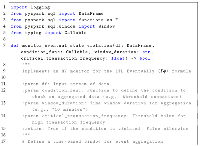
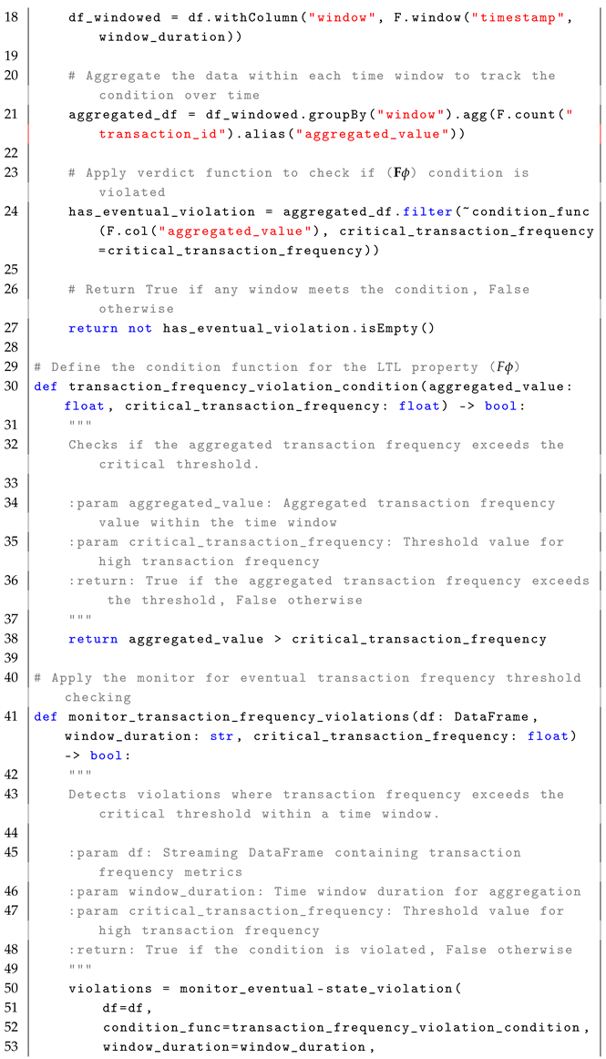
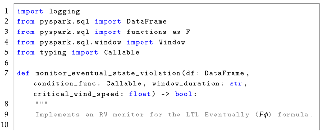
4.2. Eventually Operator ($F\varphi$)

The formula $F\varphi$ checks whether a given condition $\varphi$ will hold at some point in the future, which means that there exists a time $j\ge i$ where $\phi$ is true. The formal semantics of $F\varphi$ is defined as:

$$\sigma ,i\vDash F\varphi \iff \exists j\ge i:\sigma ,j\vDash \varphi$$

(8)

In simple terms, $F\varphi$ means that for a condition $\varphi$ to hold at the current time step i, it must be satisfied at some future time step j, where $j\ge i$. The formula $F\varphi$ is highly relevant in real-time systems where conditions are expected to be met eventually, rather than immediately. For example, it can be used to monitor whether a critical threshold for performance metrics, such as machine vibration levels, will be exceeded within a defined time frame. In real-time stream processing, the formula $F\varphi$ enables the detection of conditions that must eventually hold within a specific time window in the event stream, as described in the reference monitor approach Algorithm 2.

The monitoring process for the $F\varphi$ formula follows a stateless interpretation, where each event in the stream is treated independently to check whether a condition is met at some point in the future. Conceptually, the set of states, Q, is represented by the rows in the EventStream, and each event is observed in relation to the events that follow it, using windows-based time to define the future context for evaluation. The initial state, $q_0$, is implicitly the first row of the DataFrame, ordered by timestamp. The trace, $\sigma$, is defined by the sequence of events or rows in the DataFrame that are observed in the system over time, with each event in the stream representing a state at a particular time stamp. The alphabet of observed events, $\sigma$, refers to structured streaming events such as sensor readings, metrics, or other data points observed in the system. This alphabet represents the set of all possible events that could occur in the stream. The transition function, $\delta$, defines how states evolve over time using windowing to capture future conditions. The verdict function, $\lambda$, filters out windows where $F\varphi$ is not satisfied.

The following pseudocode (i.e., Algorithm 2) illustrates the core concept behind monitoring violations of the $F\varphi$ condition in a stream of events.

Algorithm 2 Eventual State Violation Monitoring For LTL Formula $F\varphi$

1: Input: EventStream (DataFrame), ${\mathrm{ConditionFunction}}_{\varphi }$, WindowDuration, AdditionalParameters 2: Output: Violations (Boolean) 3: Define time-based window to aggregate events into fixed windows based on “timestamp” using WindowDuration. 4: Aggregate values to compute max(event_value) in each window. 5: for each window in EventStream (ordered by timestamp) do 6:     Evaluate aggregated condition and apply ${\mathrm{ConditionFunction}}_{\varphi }$(aggregated_value, AdditionalParameters) 7:     if ${\mathrm{ConditionFunction}}_{\varphi }$ is False then 8:         Mark window as a violation 9:     end if 10: end for 11: if any window is marked as a violation then 12:     Return True 13: else 14:     Return False 15: end if

For example, in a cloud system, services generate real-time availability status updates. It is crucial to detect whether a service will eventually become available within a defined time window (e.g., 10 min) to ensure system reliability. The LTL formula for this condition is as follows:

$$F(\mathrm{service}\_\mathrm{availability}=\mathrm{True})$$

(9)

As defined in Equation (9), the formula can be implemented in Spark by first defining the condition function to check the availability of the service within a time window. This function takes as input the aggregated service availability status (aggregated_value). If the aggregated value is False, indicating a violation, the function returns True. Otherwise, it returns False.

Next, the condition is applied within a monitoring function that detects violations of the LTL property $F\varphi$. This function processes a stream of service availability data (EventStream) and the duration of the time window (WindowDuration). It groups the events into time-based windows of duration WindowDuration. For each window, the condition function service_availability_condition(aggregated_value) is evaluated. If the condition is evaluated to False, the current window is added to the violations. The function returns the set of detected violations.

4.3. Globally Operator ($G\varphi$)

The formula $G\varphi$ enforces that a given condition $\varphi$ must remain true for all future time steps, ensuring continuous compliance. The formal semantics of $G\varphi$ is defined as:

$$\sigma ,i\vDash G\varphi \iff \forall j\ge i:\sigma ,j\vDash \varphi$$

(10)

In simple terms, $G\varphi$ means that for a condition $\varphi$ to hold at the current time step i, it must remain satisfied for all future time steps $j\ge i$. The formula $G\varphi$ is highly relevant in real-time systems, where continuous compliance with operational rules must be ensured. For example, in a factory monitoring system, $G\varphi$ can check whether machine vibrations remain within a safe range throughout the operation period. In real-time stream processing, the formula $G\varphi$ allows event-driven monitoring of conditions that must remain valid for all observed data points within a defined time window, as described in the reference monitor approach Algorithm 3.

The monitoring process for the $G\varphi$ formula follows a stateless interpretation, where each event in the stream is independently verified to ensure that the condition remains valid for all future data points. Conceptually, the set of states is represented by the rows in the EventStream, each corresponding to a potential state at a specific timestamp. The initial state, $q_0$, is implicitly the first row of the DataFrame, ordered by timestamp. The trace, $\sigma$, is defined by the sequence of events or rows in the DataFrame that are observed in the system over time, with each event in the stream representing a state at a particular time stamp. The alphabet of observed events, $\sigma$, refers to structured streaming events such as sensor readings, metrics, or other data points observed in the system. This alphabet represents the set of all possible events that could occur in the stream. The transition function, $\delta$, defines how states evolve by verifying whether the monitored condition holds in each state. The verdict function, $\lambda$, determines compliance by filtering out rows where condition $G\varphi$ is violated.

The following pseudocode (i.e., Algorithm 3) illustrates the core concept behind monitoring violations of the $G\varphi$ condition in a stream of events.

Algorithm 3 Global State Violation Monitoring for LTL Formula $G\varphi$

1: Input: EventStream (DataFrame), ${\mathrm{ConditionFunction}}_{\varphi }$, AdditionalParameters 2: Output: Violations (Boolean) 3: Filter events to identify events where ${\mathrm{ConditionFunction}}_{\varphi }$(event_value, AdditionalParameters) evaluates to False. 4: if any event violates $\varphi$ then 5:     Return True 6: else 7:     Return False 8: end if

For example, in a manufacturing setting where machines generate real-time vibration data streams, ensuring that the vibration level stays below a critical threshold is vital for operational safety. The LTL formula for this condition is as follows:

$$G(\mathrm{vibration}<\mathrm{critical}\_\mathrm{vibration}\_\mathrm{threshold})$$

(11)

As defined in Equation (11), the formula can be implemented in Spark first by defining the condition function to check the vibration level at each event. This function takes as input the observed vibration level (value) and a predefined critical vibration threshold (critical_vibration_threshold). If the vibration level is below the critical threshold, the function returns True, indicating a violation. Otherwise, it returns False.

Next, the condition is applied within a monitoring function that detects violations of the LTL property $G\varphi$. This function processes a stream of vibration data (EventStream) and the critical vibration threshold (critical_vibration_threshold). It filters the events in the stream by applying the condition function vibration_violation_condition(value, critical_vibration_threshold). If any violations are detected, a warning message is logged. The function returns the set of detected violations.

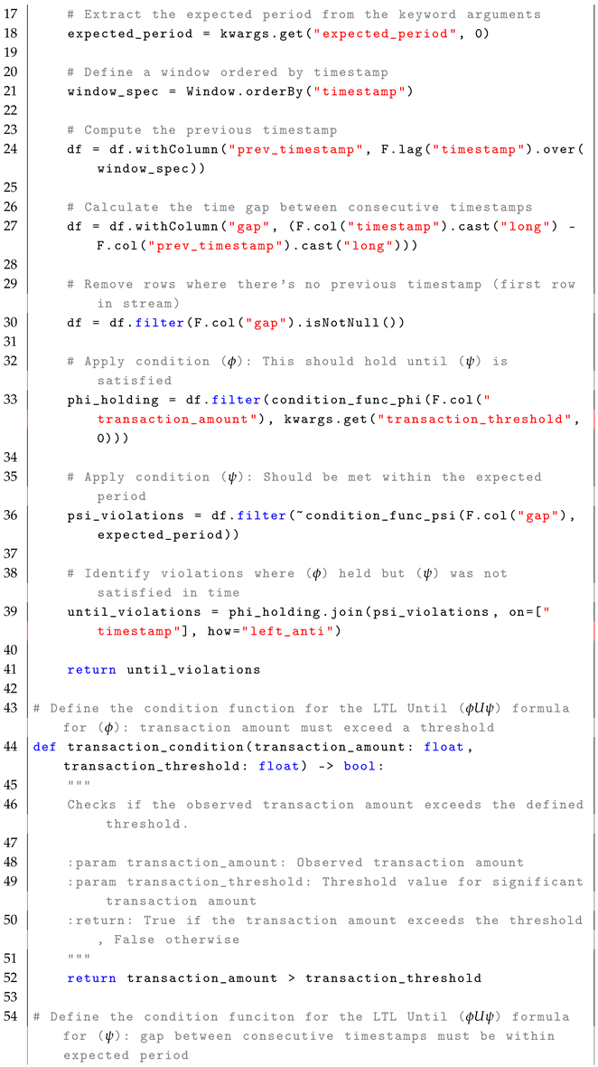
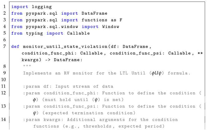
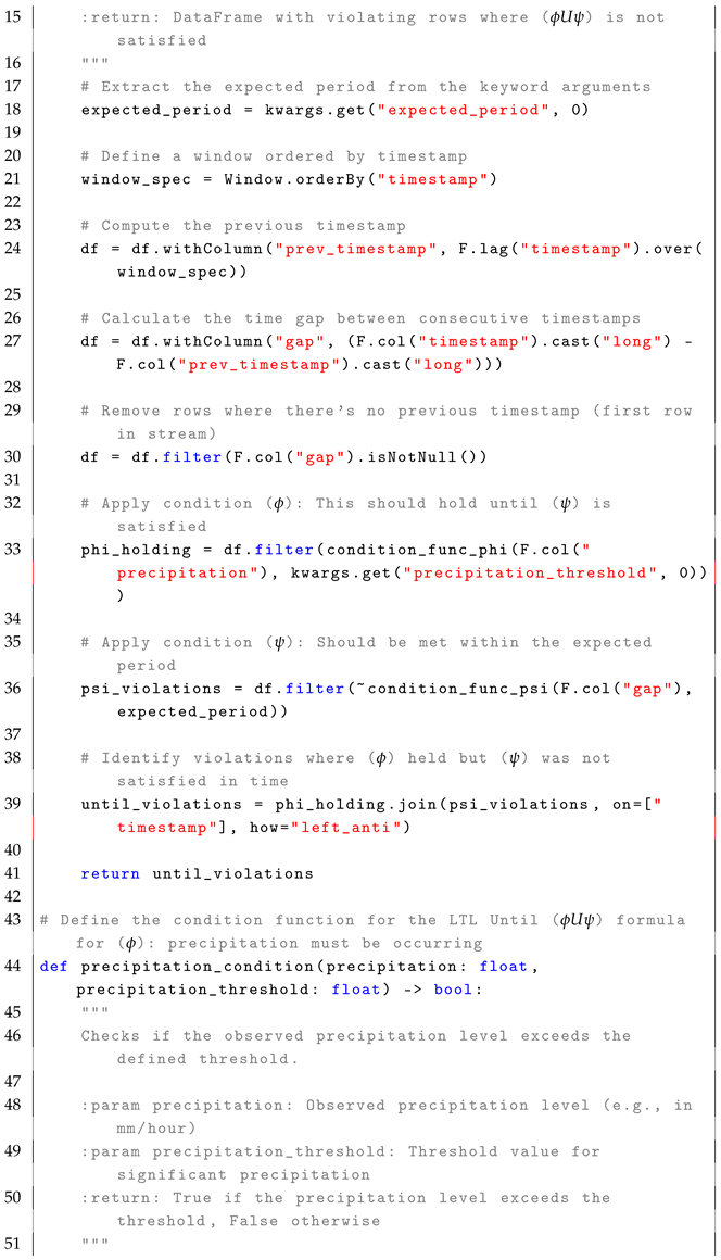
4.4. Until Operator ($\varphi U\psi$)

The formula $\varphi U\psi$ checks whether a given condition $\varphi$ must hold until condition $\psi$ becomes true at some future time. The formal semantics of $\varphi U\psi$ is defined as:

$$\sigma ,i\vDash \varphi U\psi \iff \exists j\ge i:\sigma ,j\vDash \psi \wedge \forall k,i\le k<j:\sigma ,k\vDash \varphi$$

(12)

In simple terms, $\varphi U\psi$ means that condition $\varphi$ must remain true from the current time step i until a future time step j, where $\psi$ is satisfied. The formula $\varphi U\psi$ is highly relevant in real-time systems where a condition must be maintained until a terminating event occurs. For example, in a manufacturing system, the production process must continue operating within acceptable parameters until a maintenance signal is triggered. In real-time stream processing, $\varphi U\psi$ enables the monitoring of whether a condition is continuously maintained until another condition is satisfied within a defined period, as described in the reference monitor approach Algorithm 4.

The monitoring process for the $\varphi U\psi$ formula follows a stateless interpretation, where each event in the stream is treated independently to check whether condition $\varphi$ persists until condition $\psi$ occurs. Each event is observed in relation to subsequent events, using time-based evaluation to determine whether $\psi$ is met within an expected period. Conceptually, the set of states is represented by the rows in the EventStream, where each row corresponds to an observation at a given time stamp, without explicitly maintaining past states. The initial state, $q_0$, is implicitly the first row in the DataFrame when ordered by timestamp. The trace, $\sigma$, is defined by the sequence of events or rows in the DataFrame that are observed in the system over time, with each event in the stream representing a state at a particular time stamp. The alphabet of observed events, $\sigma$, consists of structured streaming events such as sensor readings or log entries, representing the possible types of event in the system. The transition function, $\delta$, determines how events progress over time using timestamp-based tracking. The verdict function, $\lambda$, identifies violations when condition $\varphi$ is not upheld until $\psi$ is satisfied within the expected period.

The following pseudocode (i.e., Algorithm 4) illustrates the core monitoring mechanism for detecting violations of the $\varphi U\psi$ condition in a streaming environment.

Algorithm 4 Until State Violation Monitoring for LTL Formula $\varphi U\psi$

1: Input: EventStream (DataFrame), ${\mathrm{ConditionFunction}}_{\varphi }$, ${\mathrm{ConditionFunction}}_{\psi }$, AdditionalParameters 2: Output: Violations (DataFrame) 3: Define window: Order events by timestamp to process them in chronological order 4: for each event $e_t$ in EventStream (excluding the first event) do 5:     Compute time gap: $gap\leftarrow e_t.\mathtt{timestamp}-\mathtt{previous event timestamp}$ 6:     if ${\mathrm{ConditionFunction}}_{\varphi }\left(e_t\right)$ is True then 7:         Track until $\psi$ is met: Look ahead and check if ${\mathrm{ConditionFunction}}_{\psi }$ holds within the AdditionalParameters (e.g., expected_period) 8:         if ${\mathrm{ConditionFunction}}_{\psi }$ fails within the expected period then 9:            Add to violations if $\varphi$ holds but $\psi$ fails within the expected time 10:         end if 11:     end if 12: end for 13: Return Violations

For example, in a manufacturing setting, machines generate real-time vibration data streams. Ensuring that vibration levels remain below a critical threshold is vital for operational safety. The LTL formula for this condition is as follows:

$$(\mathrm{quality}>\mathrm{threshold})U\left(\mathrm{maintenance}\mathrm{required}\right)$$

(13)

As defined in Equation (13), the formula can be implemented in Spark by first defining the condition functions to check the production quality and maintenance signals. The first condition function checks whether the observed output quality (value) exceeds the predefined quality threshold (quality_threshold). If the value is greater than the threshold, the function returns True, indicating a violation. Otherwise, it returns False. The second condition function checks whether the time gap (gap) since the last maintenance signal is within the expected period (expected_period). If the gap is less than or equal to the expected period, the function returns True, indicating that the maintenance signal was in good condition. Otherwise, it returns False.

Next, conditions are applied within the monitoring function that detects violations of the LTL property $\varphi U\psi$. This function processes a stream of production quality data (EventStream), the quality threshold (quality_threshold), and the expected maintenance period (expected_period). The events are first ordered by timestamp, and the time gap between each event is computed as the difference between the current event timestamp and the previous event timestamp. The function then filters out rows where there is no previous timestamp (that is, the first row). It applies the output quality condition by filtering events where the observed quality is below the threshold. The maintenance signal condition is applied next, filtering events where the time gap exceeds the expected maintenance period. The function identifies violations by joining the filtered quality events with the maintenance signal condition, highlighting cases where the quality threshold was violated but no maintenance signal was received on time. The function returns the set of detected violations.

5. Case Study 1: Real-Time Monitoring of Financial Transaction Data Streams

To validate the generalized patterns, we applied them to a real-time financial transaction data processing scenario aimed at monitoring LTL properties, including thresholds for critical financial conditions such as transaction amount, transaction frequency, and account balance. This study addressed three key research questions related to the integration of LTL-based monitoring into Apache Spark, evaluating its impact on system performance, and assessing its scalability.

5.1. System Setup

The system is configured to support the integration of Apache Spark Streaming with a custom RV monitor. This setup is streamlined for high performance and scalability with supporting infrastructure for data ingestion and deployment. The Apache Spark pipeline processes financial transaction data streams in real time using the RV monitor to evaluate LTL properties. Detected violations are recorded and reported for immediate action. The system utilizes Kafka for high-throughput data ingestion, Airflow for workflow orchestration, and InfluxDB for time series data storage. Together, these components collectively enable efficient data flow, scheduling, and performance tracking. The system is implemented in Python and is deployed using Docker Compose, enabling scalability and simplified maintenance across distributed environments. The system setup provides the foundation for the proposed integration, demonstrating the potential of combining Spark’s distributed processing capabilities with the rigor of monitoring.

Table 2. System Configuration for Apache Spark and Kafka Brokers (Containerized Services).

Component	Configuration Detail	Resources/Settings
Spark Master	Image	bitnami/spark:3.5.2
	Master	spark-master
	CPU and Memory	2 CPUs, 2 GB Memory
Spark Workers	Image	bitnami/spark:3.5.2
	Worker-1	CPU: 2, Memory: 2 GB, Executor Memory: 2 GB
	Worker-2	CPU: 2, Memory: 2 GB, Executor Memory: 2 GB
Kafka Brokers	Image	confluentinc/cp-server:latest
	Broker-1	Partitions: 2, Replication Factor: 3
	Broker-2	Partitions: 2, Replication Factor: 3
	Broker-3	Partitions: 2, Replication Factor: 3

summarizes the key configuration details for the Apache Spark and Kafka broker components used in the system setup.

5.2. Specification of LTL Property

The monitor is designed to enforce the safety and liveness properties within the financial transaction pipeline. These properties are critical to ensuring the reliability and correctness of the system. The safety properties define thresholds to prevent fraudulent or suspicious financial activity. Violations are detected when the following limits are exceeded. A safety violation occurs if a single transaction exceeds USD 10,000 or falls below USD 1.00, potentially indicating test transactions or fraudulent micro-based transactions. High-risk behavior is flagged if an account performs more than 10 transactions within a 5 min window, which may indicate money laundering or bot activity. Account balances are monitored to ensure they remain above USD 50 to prevent overdrafts or account misuse. The liveness properties verify that the transaction updates are received consistently and that there are no data gaps, ensuring that the system maintains real-time monitoring. Transaction streams are expected to update at least every 10 min (600 s) without significant delays. The system also ensures that all transactions contain the expected attributes, preventing incomplete or corrupted records.

5.3. Mapping of LTL Formulas

In this section, we focus on the mapping of linear temporal logic (LTL) formulas to their respective safety or liveness properties, demonstrating their application in real-time data streams in Apache Spark. The goal is to provide a high-level understanding of how each formula relates to monitoring temporal properties in distributed stream processing environments. Each LTL formula is explained conceptually, showcasing its relevance and practical implications in monitoring critical system behaviors.

The formula X specifies that the condition $\varphi$ must hold in the immediate next state. It is particularly relevant in predictive scenarios, where the system monitors critical financial transitions in real time. The formula enforces safety by triggering alerts when a future violation is anticipated. In this context, the linear temporal logic (LTL) formula for transaction amount monitoring is $X(transaction\_amount>critical\_high\_amount\vee transaction\_amount<critical\_low\_amount)$, which ensures that the transaction amount exceeds or falls below predefined thresholds in the next time step. Violations of this property trigger immediate alerts, enabling rapid interventions. Similarly, formula F ensures that condition $\varphi$ will hold at some point in the future, as a liveness property guarantees that desirable or critical events will eventually be detected. 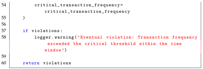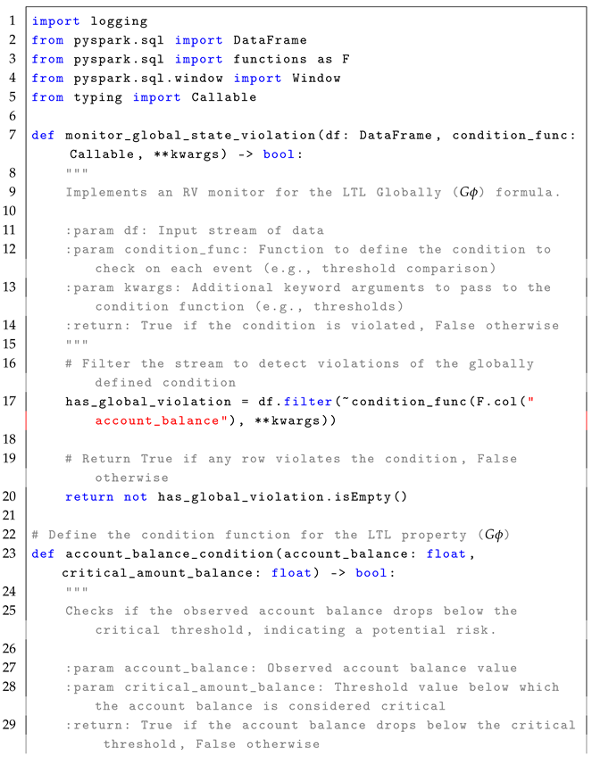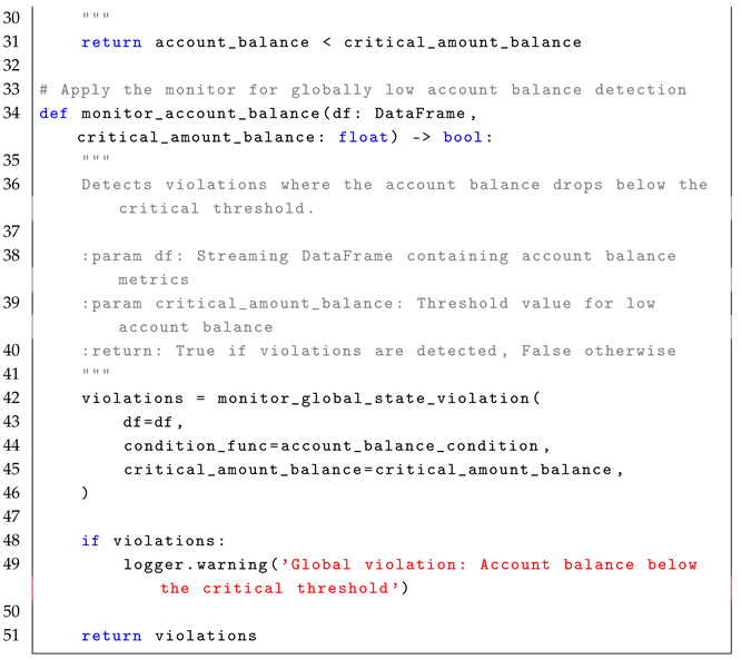The LTL formula for transaction frequency monitoring is $F(transaction\_frequency>critical\_transaction\_frequency)$, ensuring that the system eventually detects if the transaction frequency exceeds a critical threshold. The formula G enforces that the condition $\varphi$ holds throughout the entire runtime of the system, which is essential to ensure continuous safety in financial monitoring. The corresponding LTL formula for account balance monitoring is $G(account\_balance<critical\_account\_balance)$, ensuring that the account balance does not drop below critical levels at any time during the monitoring period, protecting against prolonged exposure risks. 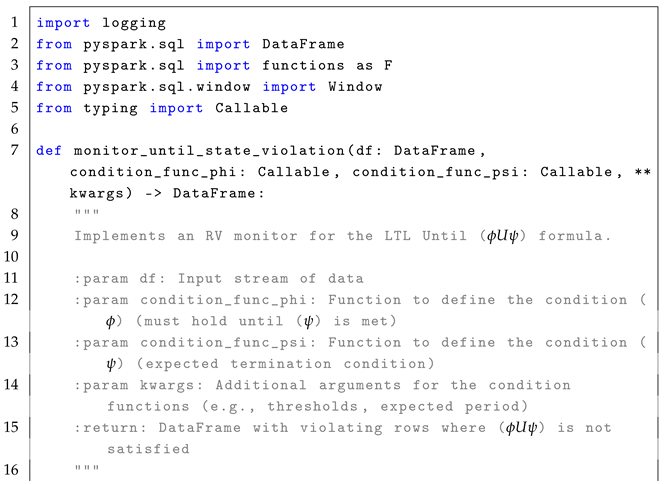Lastly, the formula $pUq$ specifies that a condition $\varphi$ must remain constant until another condition $\psi$ is met. This ensures the continuity of a condition until a triggering event occurs. The LTL formula for transaction monitoring is $(transaction\_account>0)U(data\_update=true)$, ensuring that the transaction amount persists until a data update is received, allowing continuous account tracking during system updates. Detailed implementation code snippets for these formulas are provided in Appendix A for reference.

5.4. Performance Analysis and Evaluation

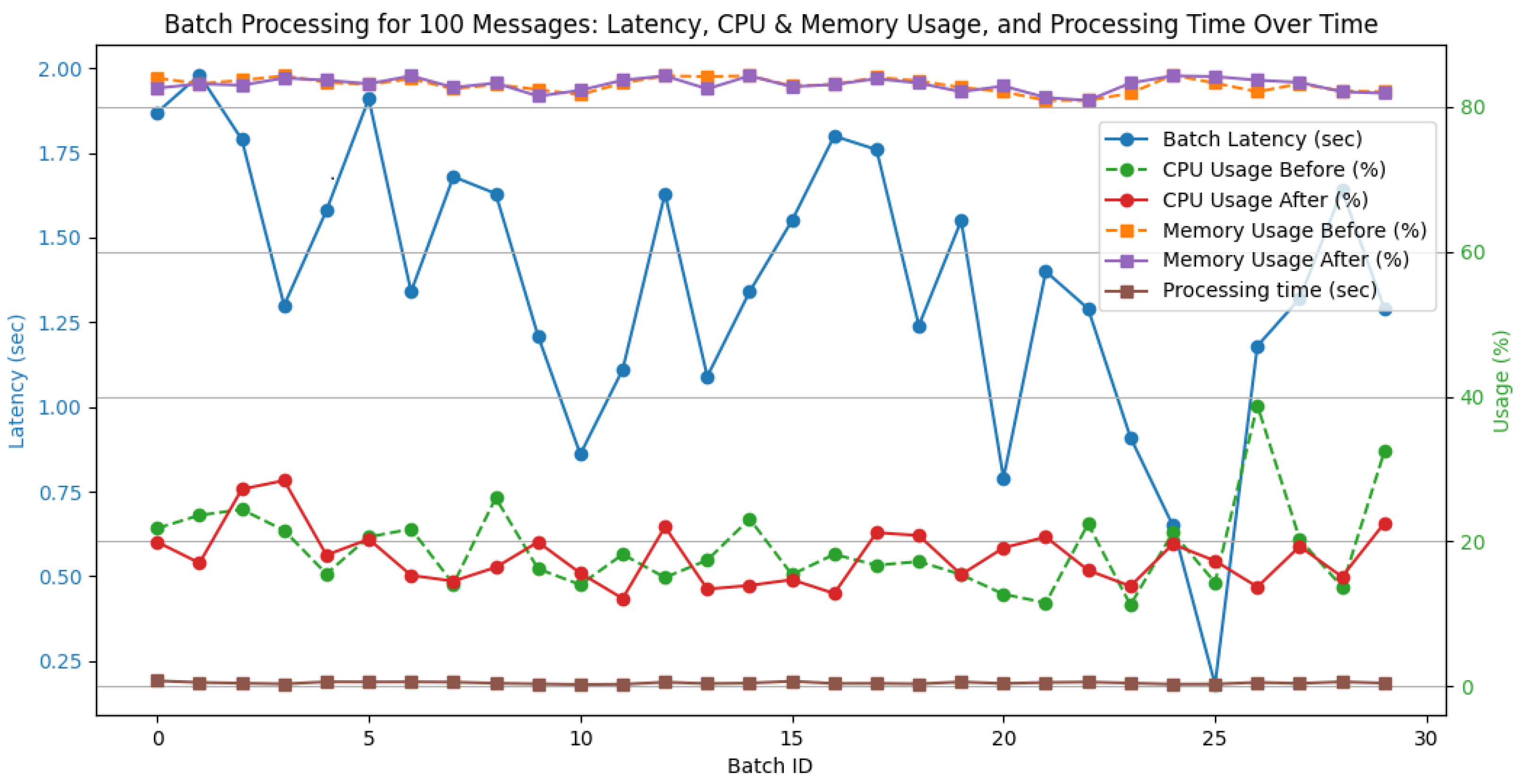
The performance of the real-time financial transaction data processing system was evaluated on three key metrics: latency, resource utilization (CPU and memory), and processing time. In addition, scalability was analyzed to assess how well the system maintained performance under increasing data loads. Each metric was tested with varying batch sizes (100, 1000, 10,000, and 100,000 messages) to evaluate the system’s ability to meet real-time processing requirements while handling large volumes of streaming data.

For a batch size of 100 messages, Apache Spark exhibited low and stable latency, with an average batch latency of 1.36 s, as shown in Figure 4. CPU and memory usage showed minimal fluctuations before and after processing, indicating efficient resource management. The processing time remained within an acceptable range, further reinforcing the system’s ability to handle small batch sizes with consistent performance and low overhead.

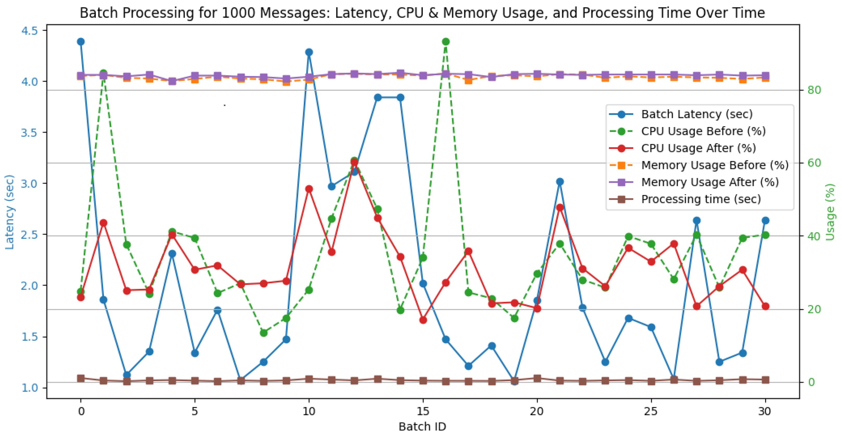
For a batch size of 1000 messages, Apache Spark exhibited low latency, with an average latency of 2.04 s, which occasionally peaked at 5.54 s, as shown in Figure 5. CPU usage fluctuated during batch processing between 10.90% and 73.40%, stabilizing to a range of 9.50% to 46.00% after processing. Memory usage remained between 81.90% and 84.60%, showing minor variations throughout the process. The processing time per batch remained relatively low, with an average of 0.63 s, which confirms the efficiency on this scale. These results indicate that the system scales effectively to 1000 messages, with only a moderate increase in processing demands.

For a batch size of 10,000 messages, Apache Spark experienced increased latency and CPU usage, reflecting the heavier computational workload, as shown in Figure 6. The average batch latency increased to 2.94 s, with peaks reaching up to 3.99 s during periods of high load. The CPU usage fluctuated significantly, ranging from 8.90% to 85.90% before processing and 10.20% to 77.20% after processing. Despite these fluctuations, the system maintained a stable memory footprint, with usage fluctuating between 81.70% and 84.80%. The average processing time per batch increased to 0.75 s, with some batches requiring up to 1.17 s.

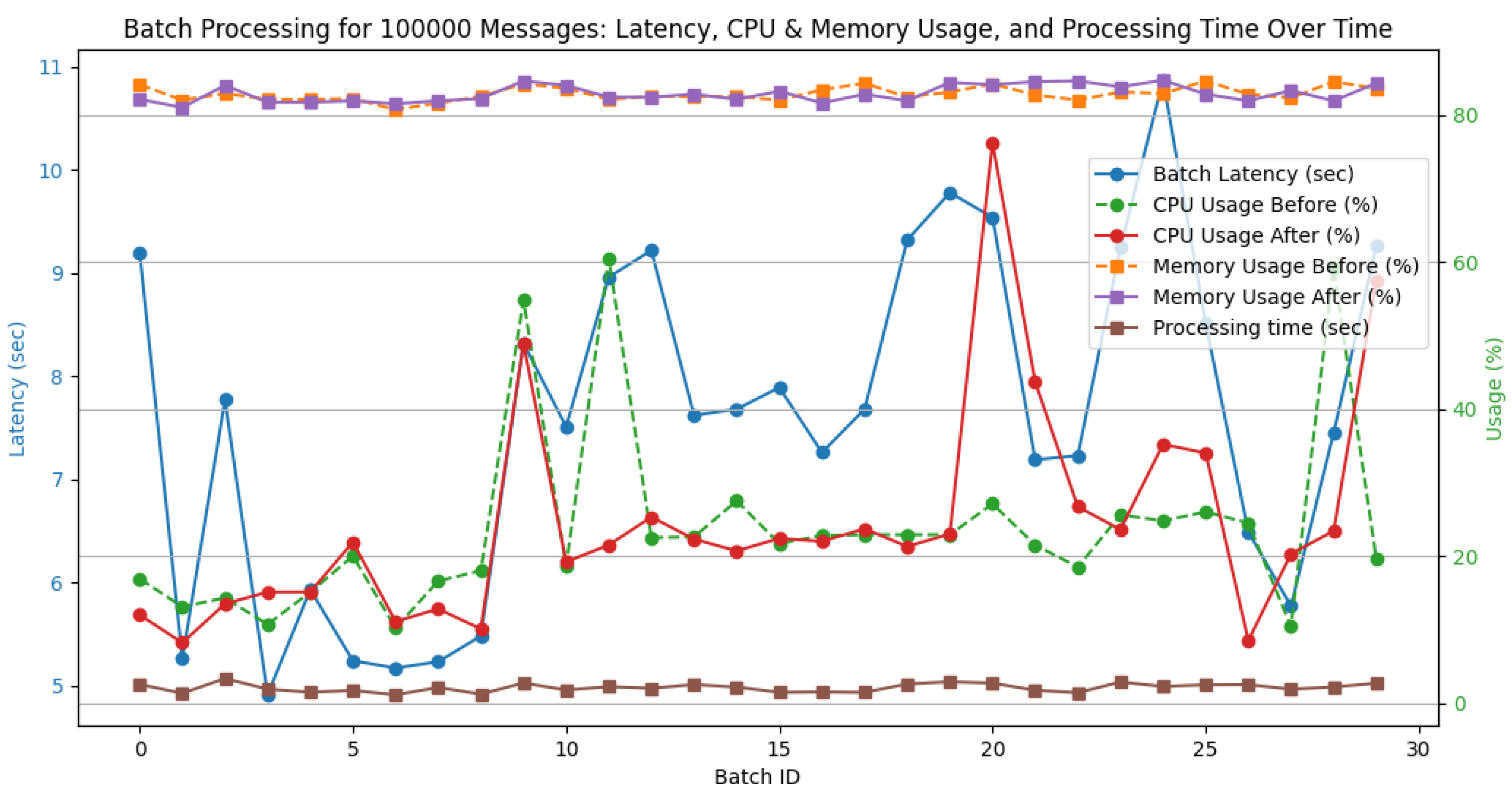
For a batch size of 100,000 messages, Apache Spark experienced increased latency and CPU usage, reflecting the heavier computational workload, as shown in Figure 7. The average batch latency increased to 7.57 s, with peaks reaching up to 10.74 s during periods of high load. The CPU usage fluctuated significantly, ranging from 10.20% to 60.50% before processing and from 8.20% to 57.50% after processing. Despite these fluctuations, the system maintained a stable memory footprint, with usage fluctuating between 80.70% and 84.70%. The average processing time per batch increased to 2.1 s, with some batches requiring up to 3.34 s.

Although latency increased with larger batch sizes, Apache Spark maintained consistent performance trends, with latency scaling predictably in relation to the increasing batch sizes. The average batch latency increased predictably from 1.36 s for (100 messages) to 2.04 s for (1000 messages) to 2.94 s for (10,000 messages) and to 7.57 s for (100,000 messages), with peaks reaching up to 10.74 s at higher loads. These results align with reported benchmarks for distributed stream processing systems [28], demonstrating that Spark’s performance is competitive with state-of-the-art systems under similar workloads.

During the case study evaluation, CPU and memory usage were closely monitored, particularly under peak load conditions. For 100-message batches, CPU utilization remained stable with minimal fluctuations. For 1000-message batches, CPU usage varied between 10.90% and 73.40% before processing and stabilized at 8.9% to 85.9% after processing. For 10,000-message batches, CPU utilization showed more significant fluctuations, ranging from 10.20% to 77.20% before processing and 9.80% to 90.30% after processing. For 100,000-message batches, CPU utilization showed more significant fluctuations, ranging from 8.20% to 57.50% before processing and 80.70% to 84.70% after processing. Memory usage remained stable across all batch sizes, fluctuating between 82.80% and 85.30%, indicating efficient resource management [28].

The scalability of the system was assessed by gradually increasing the data ingestion rate and scaling the Spark worker nodes. Apache Spark effectively maintained sub-5 s latencies for large batch sizes, ensuring timely anomaly detection and responsiveness under load [28]. Even with 100,000-message batches, the system maintained an average latency of 7.57 s, with a peak reaching 10.74 s, which remains within an acceptable range for real-time analytics. Across different configurations, Spark consistently achieved sub-2 s latencies for smaller batch sizes, reinforcing its ability to handle varying workloads without significant performance degradation.

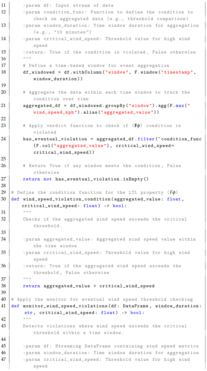
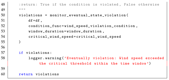
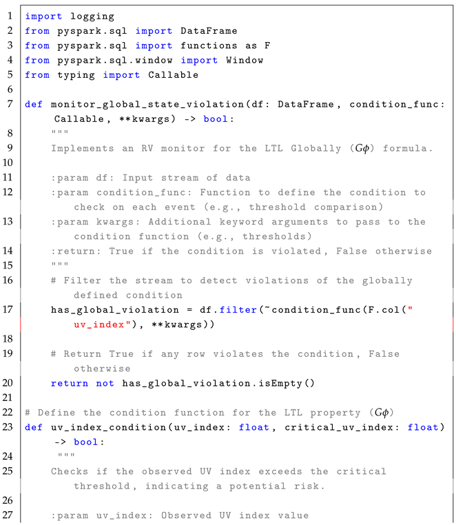
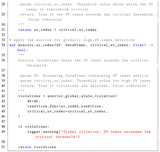
6. Case Study 2: Real-Time Monitoring of Weather Data Streams

To validate the generalized patterns, we applied them to a real-time weather data processing scenario aimed at monitoring LTL properties, including thresholds for critical weather conditions such as temperature and wind speed. This study addressed three key research questions related to the integration of LTL-based monitoring into Apache Spark, evaluating its impact on system performance, and assessing its scalability.

6.1. System Setup

The system setup follows the same configuration detailed in the first case study, integrating Apache Spark Streaming with a custom RV monitor to evaluate LTL properties in real time. The setup ensures efficient data ingestion via Kafka, workflow orchestration through Airflow, and time series data storage using InfluxDB. The deployment utilizes Docker Compose for scalability and simplified maintenance. Table 2 in the first case study provides the full configuration details for Apache Spark and Kafka brokers.

6.2. Specification of LTL Property

The monitor is designed to enforce the safety and liveness properties within the weather data pipeline. These properties are critical to ensure the reliability and correctness of the system. The safety properties define thresholds to prevent undesirable situations, such as severe weather conditions. Violations are detected when the following limits are exceeded. A safety violation occurs if the temperature rises above 35 °C or drops below 10 °C. Hazardous conditions are highlighted if wind speeds exceed 50 km/h. UV exposure levels are monitored to ensure that they remain below 8. The liveness properties verify that the system consistently delivers updates and avoids data gaps, ensuring eventual data availability. Data streams are verified to provide updates every 10 min (600 s) without interruptions. The system also ensures that precipitation data are always accessible, maintaining a complete and expected attribute set.

6.3. Mapping of LTL Formulas

This section focuses on the mapping of linear temporal logic (LTL) formulas to their respective safety or liveness properties, demonstrating their application in real-time data streams in Apache Spark. The goal is to provide a high-level understanding of how each formula relates to monitoring temporal properties in distributed stream processing environments. Each LTL formula is explained conceptually, showcasing its relevance and practical implications in monitoring critical system behaviors.

The formula X specifies that the condition $\varphi$ must hold in the immediate next state. It is particularly relevant in predictive scenarios, where the system monitors critical financial transitions in real time. The formula enforces safety by triggering alerts when a future violation is anticipated. In this context, the linear temporal logic (LTL) formula for temperature monitoring is $X(temperature>critical\_high\_temp\vee temperature<critical\_low\_temp)$, which ensures that the temperature exceeds or falls below predefined thresholds in the next time step. Violations of this property trigger immediate alerts, enabling rapid interventions. Similarly, formula F ensures that condition $\varphi$ will hold at some point in the future, as a liveness property, guarantees that desirable or critical events will eventually be detected. The LTL formula for transaction frequency monitoring is $F(wind\_speed>critical\_wind\_speed)$, ensuring that the system eventually detects if the wind speed exceeds a critical threshold. The formula G enforces that the condition $\varphi$ holds throughout the entire runtime of the system, which is essential to ensure continuous safety in financial monitoring. The corresponding LTL formula for the monitoring of the UV index is $G(un\_index>critical\_un\_index)$, ensuring that the account balance does not drop below critical levels at any time during the monitoring period, protecting against prolonged exposure risks. Lastly, the formula $pUq$ specifies that a condition $\varphi$ must remain constant until another condition $\psi$ is met. This ensures the continuity of a condition until a triggering event occurs. The LTL formula for transaction monitoring is $(precipitation>0)U(data\_update=true)$, ensuring that precipitation persists until a data update is received, allowing continuous account tracking during system updates. Detailed implementation code snippets for these formulas are provided in Appendix B for reference.

6.4. Performance Analysis and Evaluation

The performance of the real-time weather data processing system was evaluated on three key metrics: latency, resource utilization (CPU and memory), and processing time. In addition, scalability was analyzed to assess how well the system maintained performance under increasing data loads. Each metric was tested with varying batch sizes (100, 1000, 10,000, and 100,000 messages) to evaluate the system’s ability to meet real-time processing requirements while handling large volumes of streaming data.

For a batch size of 100 messages, Apache Spark exhibited low and stable latency, with an average batch latency of 1.14 s, as shown in Figure 8. CPU and memory usage showed minimal fluctuations before and after processing, indicating efficient resource management. Processing time remained within an acceptable range, further reinforcing the system’s ability to handle small batch sizes with consistent performance and low overhead.

For a batch size of 1000 messages, Apache Spark exhibited low latency, with an average latency of 2.28 s, which occasionally peaked at 4.39 s, as shown in Figure 9. CPU usage fluctuated during batch processing between 24.90% and 93.20%, stabilizing to a range of 17.10% to 53.00% after processing. Memory usage remained between 82.00% and 84.40%, showing minor variations throughout the process. The processing time per batch remained relatively low, with an average of 0.49 s, which confirms the efficiency on this scale. These results indicate that the system scales effectively to 1000 messages, with only a moderate increase in processing demands.

For a batch size of 10,000 messages, Apache Spark experienced increased latency and CPU usage, reflecting the heavier computational workload, as shown in Figure 10. The average batch latency increased to 3.35 s, with peaks reaching up to 7.55 s during periods of high load. The CPU usage fluctuated significantly, ranging from 10.60% to 85.80% before processing and 9.80% to 90.30% after processing. Despite these fluctuations, the system maintained a stable memory footprint, with usage fluctuating between 83.20% and 84.70%. The average processing time per batch increased to 0.94 s, with some batches requiring up to 1.81 s.

For a batch size of 100,000 messages, Apache Spark experienced increased latency and CPU usage, reflecting the heavier computational workload, as shown in Figure 11. The average batch latency increased to 8.85 s, with peaks reaching up to 10.74 s during periods of high load. The CPU usage fluctuated significantly, ranging from 14.2% to 84.5% before processing and from 9.9% to 91.5% after processing. Despite these fluctuations, the system maintained a stable memory footprint, with usage fluctuating between 82.8% and 85.3%. The average processing time per batch increased to 2.28 s, with some batches requiring up to 3.70 s.

Although latency increased with larger batch sizes, Apache Spark maintained consistent performance trends, with latency scaling predictably in relation to the increasing batch sizes. The average batch latency increased predictably from 1.14 s (100 messages) to 2.28 s (1000 messages) to 3.35 s (10,000 messages) and to 8.85 s (100,000 messages), with peaks reaching 10.74 s at higher loads. These results align with reported benchmarks for distributed stream processing systems [28], demonstrating that Spark’s performance is competitive with state-of-the-art systems under similar workloads.

During the case study evaluation, CPU and memory usage were closely monitored, particularly under peak load conditions. For 100-message batches, CPU utilization remained stable with minimal fluctuations. For 1000-message batches, CPU usage varied between 24.90% and 93.20% before processing and stabilized at 17.10% to 53.00% after processing. For 10,000-message batches, CPU utilization showed more significant fluctuations, ranging from 10.60% to 85.80% before processing and 9.80% to 90.30% after processing. For 100,000-message batches, CPU utilization showed more significant fluctuations, ranging from 14.20% to 84.50% before processing and 9.90% to 91.50% after processing. Memory usage remained stable across all batch sizes, fluctuating between 82.80% and 85.30%, indicating efficient resource management [28]. The scalability of the system was assessed by gradually increasing the data ingestion rate and scaling the Spark worker nodes. Apache Spark effectively maintained sub-5-second latencies for large batch sizes, ensuring timely anomaly detection and responsiveness under load [28]. Even with 100,000-message batches, the system maintained an average 8.52 s latency, with peak delays of 10.74 s, which remains within an acceptable range for real-time analytics. Across different configurations, Spark consistently achieved sub-2 s latencies for smaller batch sizes, reinforcing its ability to handle varying workloads without significant performance degradation.

7. Limitations

The proposed framework for real-time monitoring of LTL properties in distributed stream processing applications offers several advantages; however, it also presents certain limitations. First, scalability may become a concern as the volume of data grows and real-time monitoring could incur resource overhead that affects system performance, particularly in large-scale environments. In addition, the complexity of LTL formulas could impact verification performance, especially for more complex temporal properties, leading to potential bottlenecks in resource-constrained settings. Another limitation is the fault tolerance aspect of the approach. Although the system benefits from the robustness of distributed systems, ensuring accurate LTL monitoring during node failures or network disruptions may require further investigation.

The framework’s focus on Apache Spark limits its immediate applicability to other stream processing frameworks. Adapting it to platforms such as Apache Flink or Kafka Streams would require additional validation due to architectural differences in API design, state management, and check-pointing mechanisms. For example, Apache Flink’s stateful stream processing and fault tolerance model introduce challenges in integrating real-time LTL monitoring, while Kafka Streams’ close integration with Kafka’s messaging system may necessitate modifications to the monitoring logic. Addressing these differences will be a crucial aspect of future work to ensure cross-platform compatibility.

A key limitation of this study is the absence of direct experimental comparisons with existing research. Unlike traditional stream processing benchmarks, real-time verification of LTL properties lacks well-established performance baselines, making it difficult to objectively evaluate improvements. Future research should focus on defining standardized benchmarks and conducting comparative experiments across multiple frameworks, particularly Apache Flink and Kafka Streams, to assess trade-offs in latency, throughput, and resource utilization.

Furthermore, while the proposed method ensures low latency, the trade-offs between latency and throughput need to be considered, particularly in large-scale or production environments. The case study used for validation is based on financial transaction data, and additional research is required to evaluate the generalization of the framework to other domains, such as financial systems, sensor networks, or social media applications. The dependency on the Spark configuration also introduces variability in performance, and the real-time performance of the framework in a fully deployed production environment remains an open question. In terms of temporal property specification, while the framework supports a range of LTL properties, the complexity of formulating and specifying intricate temporal relationships remains a challenge. Future work will focus on expanding the evaluation to diverse use cases and exploring further optimizations for handling complex LTL formulas, improving fault tolerance, and achieving cross-platform compatibility through benchmarking against alternative frameworks.

8. Conclusions

The case study emphasizes the rationale for selecting Apache Spark as the primary framework, exploring the implications of implementing LTL monitoring in distributed stream processing, and discussing the constraints of generalizing the findings. Spark was chosen for its robustness in stream processing, its compatibility with distributed computing environments, and its mature ecosystem [13,28]. Although its microbatch processing model does not achieve true real-time processing, it provides stable latency, which is crucial for detecting time-sensitive violations specified by LTL properties. Furthermore, integration of Spark with tools such as Kafka and InfluxDB facilitates efficient data ingestion, processing, and storage, meeting the specific requirements of our study. The integration of LTL-based monitoring through a custom runtime verification (RV) monitor demonstrated how safety and liveness properties could be applied in real-time stream processing. The system successfully monitored financial transaction metrics, such as amount, frequency, and account balance, as well as monitored weather data metrics, such as temperature, wind speed, UV index, in real time, embedding LTL formulas directly into Spark’s processing pipeline. This setup ensured continuous compliance verification for time-sensitive properties, which is essential for safety-critical applications like disaster management.

The implemented framework showed good scalability when processing larger data volumes. Despite the additional processing required by LTL monitoring, Apache Spark was able to handle larger batches (up to 100,000 messages) without significant performance degradation. The latency increased proportionally with batch size but remained within acceptable limits for real-time processing. Furthermore, Spark’s ability to scale horizontally with additional worker nodes allowed the system to maintain performance even under high-load conditions, making it a suitable choice for real-time monitoring in high-throughput applications. However, a significant aspect that requires further research is the comparative evaluation of this approach with other stream processing frameworks. Future work will focus on benchmarking the proposed framework against Apache Flink, Kafka Streams, and other streaming engines to assess factors such as latency, throughput, and resource utilization. Establishing standardized testing methodologies for LTL monitoring will improve the generalization of this approach in different real-time applications. Furthermore, future enhancements will explore optimizations to improve responsiveness to dynamic data conditions and extend the framework to support diverse domains beyond financial transactions and weather data. In general, this study demonstrates the feasibility of integrating LTL-based runtime verification into distributed stream processing and highlights the need for further research to refine its performance, scalability, and cross-platform applicability.