Assessment of Movement Disorders in the Elderly Based on Skeletal Action Recognition

Abstract

With the global population aging, promoting healthy aging has become a critical societal objective. Movement disorders, which include age-related motor decline and neurodegenerative diseases such as Parkinson’s disease, significantly impair quality of life and impose substantial healthcare burdens. Early detection and intervention are crucial, yet current assessment methods primarily rely on subjective questionnaires and physical examinations, which are inefficient, resource-intensive, and lack standardization. To address these challenges, this study proposes a novel movement disorder assessment algorithm that leverages object detection, pose estimation, and action recognition techniques. By exploiting the differences in gait-related stability, coordination, and muscle activity between individuals with movement disorders and healthy individuals, the proposed algorithm employs a two-stage approach: (1) a keypoint extraction algorithm composed of the object detection algorithm and the pose estimation algorithm and (2) an improved action recognition algorithm based on the spatial–temporal graph convolutional network (ST-GCN), which incorporates a data-dependent adjacency matrix, multi-scale temporal window transformation, multimodal aggregation, and contrastive learning for precise classification. Experimental results show a 10.24% accuracy improvement over ST-GCN, achieving an accuracy of 82.03%. This method offers a more efficient, convenient, and scalable alternative to traditional approaches, providing a valuable foundation for intelligent elderly care and future research in movement disorder diagnostics.

1. Introduction

The global trend of population aging, particularly in countries like China and Japan, has become increasingly pronounced, bringing attention to the unique health challenges faced by the elderly. Among these challenges, neurodegenerative diseases, which primarily affect the brain and nervous system, are of significant concern. These diseases are marked by the degeneration and death of neurons, leading to a gradual decline in various cognitive and motor functions, including memory, thinking, and physical abilities [1]. Notably, diseases that severely impair motor function, such as Parkinson’s disease, Huntington’s disease, and motor neuron disease, are associated with symptoms like bradykinesia, tremors, and gait disturbances [2]. These motor deficits, collectively known as movement disorders, are particularly prevalent in older adults with reduced physical activity, significantly impairing basic daily tasks like walking, standing, sitting, and turning. Furthermore, numerous studies have demonstrated a strong link between movement disorders and an increased risk of falls, a major concern for the elderly population [3]. In China alone, approximately 104,000 fatal falls occur annually among individuals aged 65 and older [4], making falls the second leading cause of unintentional injury-related deaths, after road traffic accidents [5]. While aging is a superficial trigger for this increased risk, the underlying causes are twofold: first, age-related physiological changes, such as slower and stiffer movements and unstable gait, heighten the likelihood of falls; second, the increased susceptibility to neurodegenerative diseases, particularly motor disorders like Parkinson’s disease, further exacerbates this risk [6].

This study presents an in-depth analysis of the external manifestations of movement disorders, highlighting the significant relationship between these disorders and gait. Research has shown that diminished motor abilities often result in gait abnormalities, such as slower walking speed, increased step width, uneven step length, and frequent pauses during ambulation [7,8]. Additionally, movement disorders can lead to postural instability and impaired motor functions, manifesting as body sway or tilting while standing or sitting. These impairments can also affect the ability to perform daily activities that require balance, such as standing up, climbing stairs, and turning in place [9]. These external manifestations are commonly reflected in various assessment scales, including the Berg Balance Scale (BBS) [10], the Motor Assessment Scale (MAS) [11], and the Tinetti mobility test [12], all of which evaluate gait-related movements, such as independent walking, bipedal standing, standing up and sitting down, and turning. The evaluation criteria of these scales primarily focus on the stability of posture without assistance, the time taken to complete specific tasks, and the duration for which these tasks can be sustained. Consequently, these scales provide clinicians with relatively objective results derived from both experiential knowledge and quantitative evaluation criteria.

However, existing scale evaluation methods exhibit limitations, including their singular format, lack of direct measurement of actual motor ability, and the potential for participant bias due to unreliable memory or intentional misreporting. These factors compromise the accuracy and stability of the evaluation results. Although simple action testing improves accuracy, it requires significant medical human resources and is often cumbersome and time-consuming. Professional equipment offers the highest measurement precision, but is constrained by site limitations, high costs, and the consumption of valuable medical equipment resources, which hinders its widespread adoption for screening movement disorders in the elderly [13]. Given these challenges, this study proposes an in-depth exploration of skeleton-based action recognition algorithms for evaluating movement disorders through video analysis. By extracting the spatiotemporal features of elderly gait movements and analyzing the motion information, the proposed method aims to provide more efficient, accurate, and scalable evaluation and classification of movement disorders. This study specifically investigates the external manifestations of movement disorders, with a focus on gait-related movements. Through collaboration with professional clinicians, the most representative movements were selected to construct an RGB video dataset for the assessment of movement disorders. By optimizing human object detection and posture estimation techniques, bone keypoint sequences were efficiently extracted, and motion recognition algorithms were developed to assess the presence or absence of movement disorders.

The main contributions of this study are as follows:

• Three actions, including walking back and forth, standing up and sitting down, and turning around in place, were designed for data collection in movement disorder assessment. Standardized and effective dataset collection experiments were conducted, with professional clinical assessments used as labels for the data;
• The proposed motion disorder assessment algorithm achieved an accuracy of 82.03% on the collected test dataset, outperforming the original ST-GCN by 10.24% and SkeletonGCL by 4.32%;
• This study further explored the feasibility of applying skeleton-based action recognition methods in fine-grained movement disorder assessments, offering valuable insights and a reference for the development of alternative methods in this field.

2. Related Works

Current assessment methods for movement disorders can be categorized into three main types: questionnaire-based assessments, comprehensive assessments using simple instruments or movements, and in-depth analyses using professional equipment. Questionnaire-based assessments, such as the fall risk questioning method [14] proposed by the British American Elderly Association for individuals aged 65 and above, offer a simple approach. A more detailed and professional method is the Morse Fall Scale (MFS) [15] developed by the University of Pennsylvania, which evaluates six aspects of movement. Additionally, Dr. Hendrich’s HFRM II Fall Risk Model [16] provides a more comprehensive assessment than the MFS, while the Johns Hopkins fall risk assessment tool (JHFRAT) scale, designed for hospitalized patients, focuses on inpatient nursing conditions and movement disorder risk [17]. Comprehensive assessments using simple instruments or movements involve tasks such as the classic 4-step balance test [18], commonly used in clinical settings to evaluate motor abilities through hierarchical movement tasks. Other relatively simple tests include the standing walking timing test [19] and the 30-second sitting–standing counting test [20]. In-depth assessments using professional equipment focus on more precise measurements of gait and motor function, such as the Tinetti Performance-Oriented Mobility Assessment [12], Berg Balance Test [21], and Dynamic Gait Index [22], as well as force-measuring platforms and plantar pressure distribution systems that quantify biomechanical parameters [23]. With advancements in sensor technologies, research into gait analysis using imaging and wearable technologies has gained much attention [24,25].

While the goal of movement disorder assessments is to detect related issues early in the elderly, current methods are hindered by subjective factors, time-consuming procedures, and cumbersome questionnaires. Simple equipment and movement tests place a heavy demand on medical resources, and professional assessments require specialized equipment and settings. Machine vision-based methods offer a promising solution, reducing the burden on healthcare systems while maintaining objectivity and accuracy. This approach can be implemented in hospitals, communities, and homes, enabling convenient, rapid testing for the elderly. Machine vision methods work by first determining the subject’s position in the video frame using human object detection, eliminating irrelevant background information. Then, human pose estimation extracts keypoint coordinates, preserving crucial movement information while discarding redundant details. This method significantly improves the extraction of relevant data compared to directly processing RGB videos. Finally, skeletal keypoint sequences are used for action recognition and classification, determining the presence of movement impairments based on the subject’s ability to complete specific actions.

In object detection, faster region-based convolutional neural networks (R-CNNs) [26] efficiently generate object proposal boxes by introducing a Region Proposal Network (RPN), which enhances accuracy by refining candidate regions. You Only Look Once (YOLO) [27], a real-time object detection algorithm, reformulates object detection as a regression problem, enabling fast and efficient predictions. The Single Shot MultiBox Detector (SSD) [28] achieves multi-scale object detection by leveraging feature maps at different levels, improving its capability to detect objects of varying sizes. In human pose estimation, OpenPose [29] can simultaneously detect keypoints of multiple individuals by employing a combination of convolutional neural networks (CNNs) and recurrent neural networks (RNNs). The Hourglass Network [30] adopts a bottom-up and top-down approach to refine feature representations at different resolutions, enhancing keypoint localization accuracy. The High Resolution Network (HRNet) [31], a high-resolution network architecture, maintains high-resolution representations throughout the model, allowing for the extraction and fusion of spatial features from different resolutions while preserving critical spatial information. Simple Coordinate Classification (SimCC) [32] simplifies human pose estimation by transforming it into a keypoint coordinate regression problem, significantly reducing model complexity and computational overhead. In skeleton-based action recognition, early approaches utilized long short-term memory (LSTM) networks to capture the spatiotemporal dependencies of keypoint sequences, thereby improving action recognition performance [33]. The introduction of spatial–temporal graph convolutional networks (ST-GCNs) [34] has revolutionized traditional CNN-based methods by modeling skeletal keypoints as nodes in a graph. ST-GCN defines adjacency relationships based on the connectivity of keypoints and extends conventional convolutional operations to graph structures, facilitating efficient learning and recognition of complex human actions. Pose estimation has demonstrated strong performance in movement assessment and has garnered significant attention from researchers in rehabilitation and telerehabilitation. Kim et al. [35] proposed a transformer-based 3D pose estimation model with rehabilitation-focused tokens, improving temporal consistency and achieving 49.0 mm PA-MPJPE on 3DPW. Latreche et al. [36] developed an AI model and web app to remotely track patient rehabilitation progress through motion analysis. To address rehabilitation monitoring challenges, Aguilar-Ortega et al. [37] evaluated pose estimation methods on a new multi-view dataset, showing 2D analysis suffices for joint angle measurement.

Building on the aforementioned research, the movement impairment assessment proposed in this study utilizes RGB video recordings of elderly individuals performing specific actions as input. These videos are processed to extract skeletal keypoint sequences, from which spatial and temporal features are analyzed. However, existing action recognition algorithms are primarily designed for coarse-grained public datasets, where the distinctions between different actions are relatively large. In contrast, the difference in skeletal keypoint sequences between individuals with normal and impaired motor function performing the same action is subtle, making this a fine-grained action recognition task. Consequently, open-source models cannot be directly applied, necessitating targeted algorithmic improvements to enhance classification accuracy. Furthermore, there are currently no publicly available video datasets specifically designed for movement disorder assessment. Most existing datasets focus on professional bioinformatics applications and are not directly applicable to this domain. Therefore, it is essential to design and implement a dedicated experimental data collection plan to facilitate model training and evaluation.

3. Datasets

Given that this study employs skeleton-based action recognition methods, the collection and construction of an early-stage motion video dataset are of critical importance, as the quality of the dataset directly impacts the effectiveness of the final model. To ensure robustness and reliability, a structured data collection plan was designed and implemented to create a specialized motion video dataset for subsequent training. The final dataset collection experiment involved three predefined actions:

• Walking back and forth over a 5-meter distance once;
• Standing up and sitting down twice without the aid of handrails;
• Turning around in place once in both the clockwise and counterclockwise directions.

The reason for choosing the three actions is mainly for several important manifestations of the decline of the elderly’s motor ability. Walking back and forth corresponds to the overall coordination of the lower limbs and arms. Standing up and sitting down mainly targets the vulnerable knee joint. Turning around in place targets the prone hip joint. The combined effect of these three actions exposes potential motor disorders. Each action was controlled to last approximately 10 s to maintain consistency, as illustrated in Figure 1. Approximately 1000 people participated in the collection of video data and all signed the consent forms, with a male-to-female ratio of about 1:1. In the end, there were more than 3000 videos with a total duration of about 500 min.

After collecting the gait action videos, direct training on the dataset is not feasible. Several preprocessing steps must be performed to convert the raw video data into a standardized, continuous, and unified sequence of skeletal keypoints before they can be utilized as input for the action recognition classification model. The overall preprocessing workflow is illustrated in Figure 2, with the detailed steps outlined as follows:

• Video Screening and Invalid Segment Removal: The original video recordings are examined to eliminate invalid segments lasting more than one second. These include instances where the subject is not actively performing an action, is out of the frame, the video quality is excessively blurry, or the subject’s lower limbs are obstructed, preventing accurate keypoint extraction.
• Human Object Detection and Pose Estimation: Once the selected video clips are finalized, human object detection and pose estimation algorithms are applied to extract skeletal keypoint sequences. Background and torso information are removed to minimize data redundancy, reduce input complexity for the action recognition model, and enhance the efficiency of subsequent spatiotemporal feature extraction.
• Interpolation for Missing Frames: To address the challenge of missing or blurred frames caused by object detection and pose estimation inaccuracies, interpolation techniques are applied to fill in missing frames with zero values, ensuring data continuity and mitigating potential adverse effects on model performance.
• Keypoint Normalization: The extracted keypoint coordinates are normalized by dividing their width and height by fixed values of 1920 and 1080, respectively. This transformation scales all coordinates within the range of 0 to 1, ensuring consistency across different video resolutions.
• Temporal Dimension Standardization: To facilitate uniform training, the time dimension size of all keypoint sequences is standardized. Specifically, all sequences are adjusted to match the longest frame length among them. Sequences with fewer frames are padded with zeros to maintain consistency in model input.

The keypoint sequence obtained through the above preprocessing is stored in the form of vectors with a shape of $(N,T,V\times C)$, where N represents the number of samples, T represents the uniform frame rate of all video samples, and V represents the number of keypoints. The COCO skeleton architecture used in this article is fixed at 17 keypoints, and C represents the feature dimension, which can be two-dimensional or three-dimensional. The dataset collected in this article is two-dimensional. The corresponding labels are also stored in tensor form, with a shape of $(N,NC)$, where $NC$ represents the final number of categories.

4. Methodologies

As previously discussed, this study adopts a skeleton-based action recognition algorithm to classify action videos and assess motion impairments. Given the fine-grained nature of the collected dataset, our research primarily focuses on enhancing action recognition algorithms to improve fine-grained action discrimination. The keypoint extraction process leverages established state-of-the-art methodologies, where human object detection is implemented using YOLOv8, and human pose estimation is conducted using SimCC. The reason for choosing YOLOv8 is that YOLO has good real-time performance, and as a relatively new architecture, v8 is mature and has excellent performance in applications, making it easy to get started. The reason for choosing SimCC is that it is a regression-based method that sacrifices less accuracy while significantly improving speed, meeting the requirements of high real-time performance. This study proposes the Spatial–Temporal Fuse Graph Contrastive Learning Network (STFGCL), which will be described in detail in the subsequent sections. The proposed method builds upon the fundamental framework of the spatial–temporal graph convolutional network (ST-GCN) and introduces optimizations tailored for fine-grained keypoint sequence datasets. Compared to the structural diagram of ST-GCN (as illustrated in Figure 3), the overall architecture is based on a series of stacked blocks for deep feature extraction.

However, a key distinction is that graph convolutional network (GCN) modal aggregation is performed prior to the first block, whereas temporal convolutional network (TCN) modal aggregation is conducted at the end of each block. In the GCN stage within each block, the traditional ST-GCN applies a 1 × 1 convolution for channel transformation on the input, followed by direct graph convolution using the adjacency matrix to generate intermediate representations. In contrast, STFGCL integrates graph convolution with an adjacency matrix alongside a multi-scale time window transformation module that operates on fused data. The outputs from these transformations are subsequently concatenated to produce the final intermediate feature representations. Furthermore, STFGCL introduces a contrastive learning strategy following the graph convolution stage, where the adjacency matrix is utilized as input to optimize fine-grained category discrimination. This approach enhances the model’s ability to distinguish subtle variations in motion patterns, thereby improving the overall effectiveness of fine-grained action recognition.

4.1. Dynamic Adjacency Matrix for Integrating Data Dependencies

ST-GCN utilizes a predefined skeletal structure as its adjacency matrix, which is based on human anatomy and aligns with the physiological structure of the human body. However, the use of a fixed adjacency matrix lacks flexibility due to its static topology and it struggles to capture deep, latent relationships between keypoints. To address these limitations, this study introduces a dynamic adjacency matrix that integrates data dependencies, enhancing adaptability and fine-grained feature representation. The improved graph convolutional layer structure is illustrated in Figure 4, with the fused adjacency matrix comprising three components:

• Prior Adjacency Matrix (A): Derived from the original skeletal structure, this matrix differs from the three predefined groups used in traditional ST-GCN. Instead of relying on fixed groupings, this study employs convolution operations to map the prior matrix into K groups, preserving its intuitive structural information while enabling the model to extend and adapt appropriately.
• Learnable Adjacency Matrix (B): This fully learnable matrix is initialized randomly and optimized through training, providing high flexibility. Since B is entirely dependent on the input dataset, it can dynamically adjust to capture task-specific keypoint relationships, particularly for the three predefined actions in this study’s dataset.
• Data-Dependent Adjacency Matrix (C): Introduced to compensate for the limitations of A and B in capturing input-specific variations, this matrix is designed to enhance fine-grained action discrimination. Specifically, two separate $1\times 1$ convolutional layers transform the channel dimension to generate two feature maps, $X_1$ and $X_2$, each containing K groups. These two feature representations are then subtracted via broadcast operations to highlight differences between keypoints within a single data instance. The resulting matrix is multiplied to amplify the weight differences before linking keypoints, allowing the model to capture subtle variations in fine-grained data. Finally, activation functions such as SoftMax or Tanh are applied to generate $C_1$ and $C_2$, which together constitute the third component of the fused adjacency matrix.

By integrating these three components, the proposed method enhances adaptability and improves the model’s ability to capture both explicit and implicit spatial relationships, leading to better performance in fine-grained movement disorder assessments.

The fusion adjacency matrix is constructed based on the three components mentioned above. However, instead of applying simple addition or averaging, it utilizes fully parameterized weights that are learned during training, as shown in Equation (1). The parameters $\alpha$, $\beta$, and $\gamma$ control the contribution of different adjacency matrices, ensuring a balanced integration. This prevents the fusion adjacency matrix from being overly biased toward either the prior information or the learned parameters, which could negatively impact training performance. The prior matrix serves as the foundational structure, with its weight fixed at 1.

$$A_f=A+\alpha \times B+\beta \times C_1+\gamma \times C_2$$

(1)

In the GCN structure, the adjacency matrix is fused with the input $X_{pre}$, which has undergone convolution for channel transformation. A residual connection is then applied to the original input to mitigate the gradient vanishing problem and accelerate model convergence. Finally, the output is obtained through a nonlinear transformation using an activation function. This output serves as a component of the overall GCN and is further fused with the results from the subsequent multi-scale time window transformation to generate the final GCN output.

4.2. Multi-Scale Time Window Transformation

ST-GCN applies a temporal convolutional network (TCN) immediately after the graph convolutional network (GCN) to extract temporal features. However, its approach to temporal feature extraction presents several key limitations: (1) GCN and TCN process features independently, leading to insufficient integration of spatial and temporal information. (2) TCN employs a sliding window approach for temporal feature extraction. While long time windows struggle to capture complex actions or subtle variations, using multiple short windows may result in the loss of essential global information. (3) The convolution kernel size in TCN remains constant, which restricts its ability to adapt to fine-grained action distinctions, making it less effective for precise motion analysis.

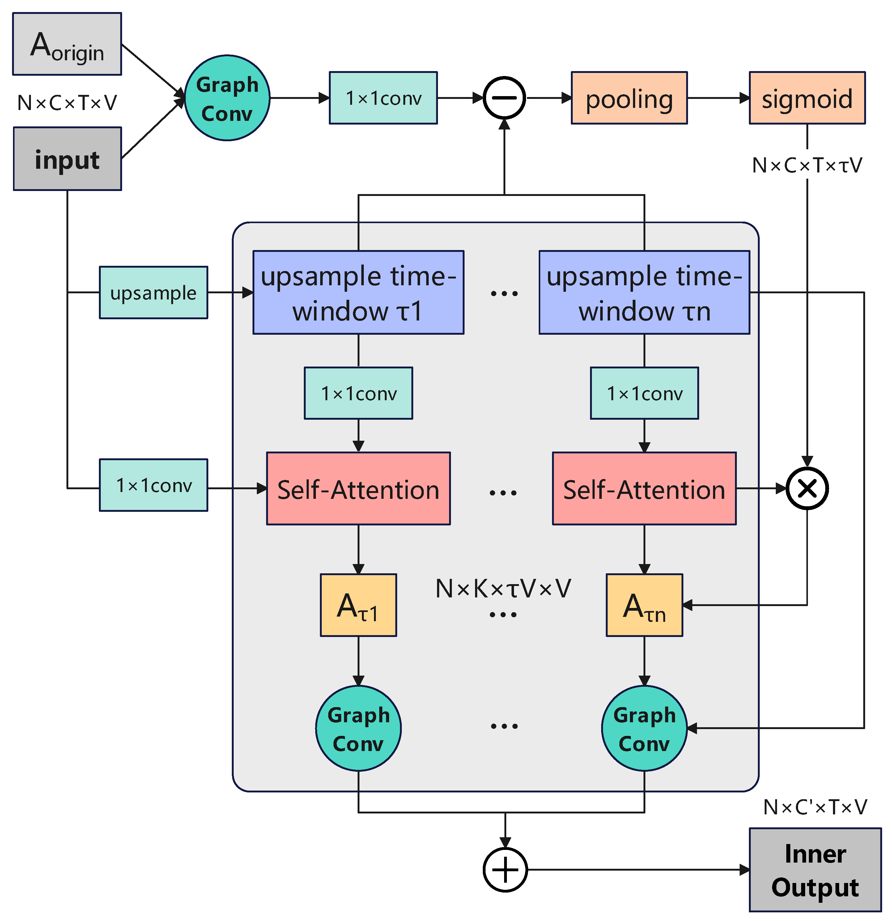
To address the aforementioned limitations, this study proposes a multi-scale time window transformation module to extract and integrate temporal features at different granularities. To enhance the exchange of spatial–temporal information, the module is integrated into the GCN by leveraging the properties of the adjacency matrix and attention mechanism. The structure of the improved GCN module is illustrated in Figure 5. In this framework, the input is upsampled to generate multi-scale time window transformation results, where the transformation scales are denoted as ${\tau }_1$ to ${\tau }_n$. Each upsampled result is represented as:

$$X_{\tau }^t=x_{t-\tau /2:t+\tau /2}\in R^{C\times \tau V}|t\in Z, 0\le t<T$$

(2)

In Equation (2), t is the time, $\tau$ is the time window size, C is the number of features, V is the number of keypoints, and T is the number of the total frames. After applying a 1 × 1 convolution, the transformed input is used as the $Query\in R^{K\times C^{\prime }\times \tau V}$ in the self-attention module. Similarly, the original input undergoes a 1 × 1 convolution and is used as the $Key\in R^{K\times C^{\prime }\times V}$. The resulting output has a structure similar to a standard adjacency matrix but includes an additional dimension corresponding to the time window transformation $\tau$. This additional dimension enables the representation of relationships between key points across a local time range, effectively capturing cross-temporal and spatial connections. Furthermore, the transformation of inputs and the introduction of a self-attention mechanism to emphasize features across different time window sizes result in an extended computational pathway. This leads to a significant loss of direct information in the final time window adjacency matrix representation. To mitigate this issue, a side branch is introduced to preserve essential information. As illustrated at the top of Figure 5, this side branch performs fast and continuous subtraction, pooling, and nonlinear sigmoid transformation. The output of this branch is denoted as $P\in R^{C\times \tau }$, representing the pooled result along the time window dimension. By expanding its dimension and replicating it according to the number of key points, $P_f\in R^{C\times \tau V}$ is obtained. $P_f$ is then element-wise multiplied with the output of the self-attention module to produce $A_{\tau }$.

4.3. Multimodal Internal Aggregation

The input data of ST-GCN consist of a sequence of skeletal keypoints, which only captures the spatial coordinates of these keypoints. However, relying solely on spatial position information may result in the omission of crucial motion characteristics, as it represents human movement purely from a spatial perspective without accounting for its temporal evolution. To address this limitation, this study introduces additional modality information to enrich the supervised data during model training, thereby enhancing the performance of fine-grained action recognition. The introduced modalities include keypoints and bone connections, which are detailed below.

The calculation method of bone connection is defined in Equation (3), where $Pair$ represents all predefined bone connections, totaling 12 segments. Each $Pair$ is a binary representation of the indices of two connected keypoints. The final bone connection features are obtained by subtracting the coordinates of the two connected keypoints $\left(X^{Pai{r}_i}\right)$ to form a vector, denoted as b. The velocity calculation is defined in Equation (4), where velocity is computed by subtracting the coordinates of keypoints in adjacent frames, using a 1-frame interval. Missing values are zero-padded for consistency. The acceleration computation is given in Equation (5), where acceleration is derived by subtracting the velocities of adjacent frames, also measured using a 1-frame interval. Missing values are similarly zero-padded for alignment. The angle mode is formulated in Equation (6), where the angles between adjacent keypoints are represented by the inverse cosine function. The bone connection source is linked to the skeleton mode, with every two connected bones forming an implicit angle. The calculation methods for angular velocity and angular acceleration follow the same approach as those for keypoint velocity and acceleration.

$$b=X^{Pair\left[0\right]}-X^{Pair\left[1\right]}, 0\le i<12$$

(3)

$$v=\left\{\begin{array}{c}{X}_{t+1}-X_t, 0\le t<T-1\hfill \\ 0, t=T-1\hfill \end{array}\right.$$

(4)

$$a=\left\{\begin{array}{c}{v}_{t+1}-v_t, 0\le t<T-1\hfill \\ 0, t=T-1\hfill \end{array}\right.$$

(5)

$$\theta =co{s}^{-1}{\displaystyle \frac{b_i·b_j}{\left|\right|b_i\left|\right|·\left|\right|b_j\left|\right|}}$$

(6)

In Equation (3), b is the bone dataset, $Pair$ is the a priori skeletal connectivity relationship, X is the keypoint dataset, and i is the index of keypoints. In Equation (4), v is the velocity dataset, t is the frame index, and T is the number of total frames. In Equation (5), a is the acceleration dataset. In Equation (5), $\theta$ is the angle dataset. To incorporate the aforementioned modalities, this study proposes fusing keypoint, keypoint velocity, and keypoint acceleration at the input stage of the graph convolutional network (GCN). 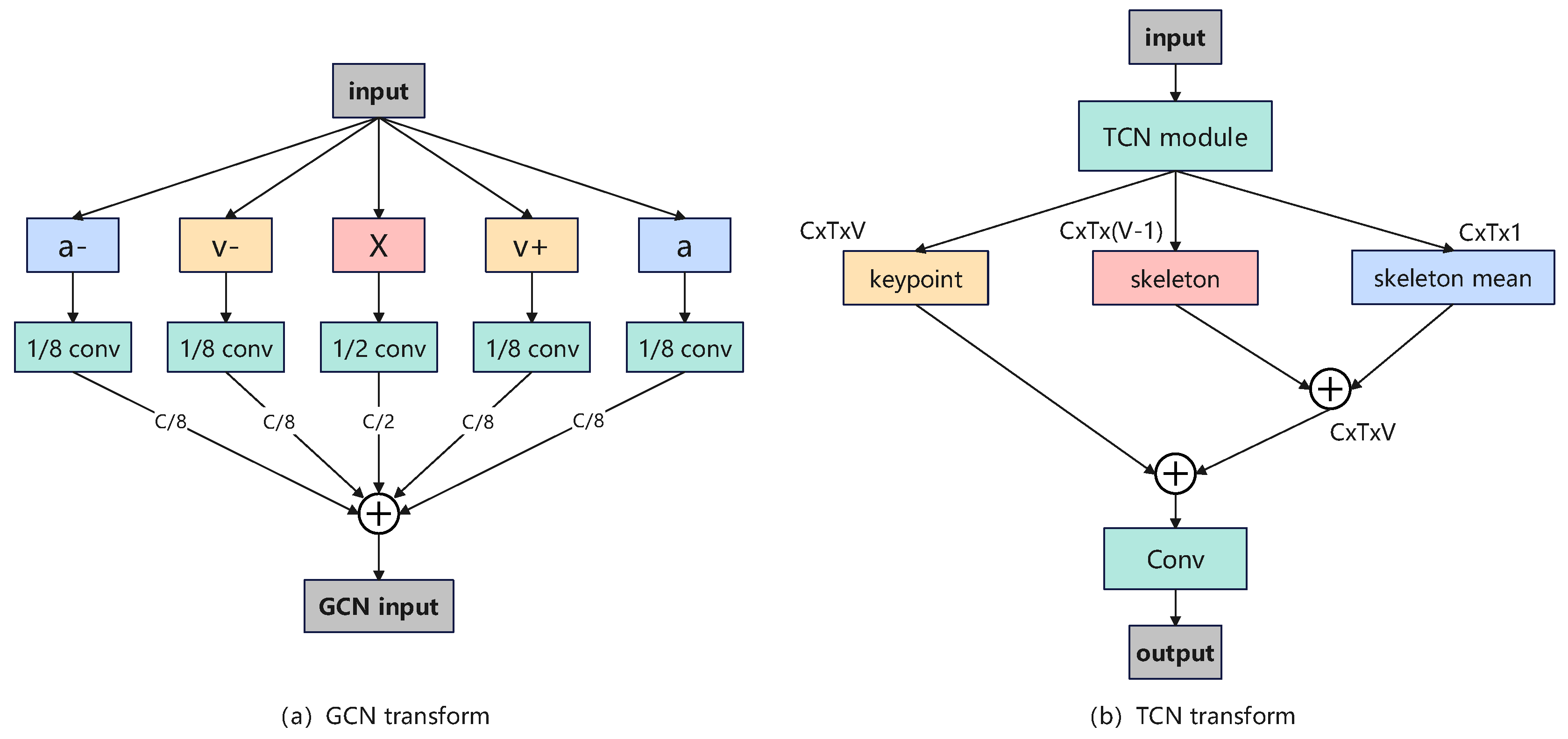The specific fusion process is illustrated in Figure 6a. As shown in the figure, the raw input is divided into five components: the original keypoint coordinates X, forward-differenced velocity $v_{+}$, backward-differenced velocity $v_{-}$, forward-differenced acceleration $a_{+}$, and backward-differenced acceleration $a_{-}$. To balance the contribution of different modalities while maintaining the feature dimension of the GCN input, X is convolved by a factor of 1/2, while the remaining modalities are convolved by a factor of 1/8. Because the acceleration and velocity are divided into positive and negative directions and the original variables should maintain a relatively large proportion, the proportions are set to 1/8 and 1/2 to keep the merged feature dimension unchanged. The outputs are then fused along the feature dimension to form the final GCN input. By integrating the directional features of forward and backward motion velocity and acceleration within the time domain, this multimodal fusion enhances intermodal information exchange within the GCN, leading to a more comprehensive representation of motion dynamics.

The multimodal fusion in the temporal convolutional network (TCN) is illustrated in Figure 6b. The intermediate module processes the input and produces an output with the shape $C\times T\times V$, representing the keypoint modality. To incorporate skeletal connectivity, the bone connection modality is derived based on the prior skeleton structure shown in Figure 6, resulting in a shape of $C\times T\times (V-1)$. Since this transformation reduces the keypoint dimension, a bone mean feature is introduced to compensate for the missing information. This is achieved by averaging the TCN intermediate output along the keypoint dimension, yielding a feature with the shape $C\times T\times 1$. The bone connection modality and the bone mean feature are then stacked and merged, followed by a weighted addition to the keypoint modality. The final fused representation undergoes convolution to produce the TCN output. The weights for this fusion process are learned during training, ensuring an adaptive balance between the bone connection modality and the bone mean information, optimizing the model’s ability to capture fine-grained motion dynamics.

4.4. Contrastive Learning Strategies

After the above optimizations, the proposed model achieves high performance on public datasets where action categories exhibit significant differentiation. However, certain limitations remain when applied to the keypoint sequence dataset constructed in this study. Specifically, the difference between normal and abnormal behaviors within the same action category is often subtle, making classification more challenging. To address this issue, this study introduces a contrastive learning strategy, a technique that enhances feature representation learning by leveraging sample relationships. The core concept is to train the model to distinguish intra-class and inter-class samples, making intra-class features more compact while increasing the separability of inter-class features. Building on the data-dependent dynamic adjacency matrix introduced in Section 4.1, this study employs it as the input to the contrastive learning module. A dedicated loss function is applied to guide the learning process of the dynamic adjacency matrix, reinforcing its ability to capture fine-grained differences in action recognition. The overall structure of the proposed method is illustrated in Figure 7.

Contrastive learning aims to enhance feature representations by maximizing intra-class similarity while increasing inter-class differentiation. However, directly using highly abstract features as benchmark samples for contrastive learning may lead to significant information loss due to multiple fusion and transformation stages in graph convolution and temporal convolution, thereby reducing their direct representativeness. To address this issue, this study adopts the adjacency matrix as the benchmark sample for contrastive learning. After graph convolution processing, the dynamic adjacency matrix and intermediate output are extracted as results. The dynamic adjacency matrix is then passed to the adjacency matrix mapping module, where it undergoes pooling, flattening, and transformation to generate a high-dimensional feature representation f with the shape $N\times C_f$. During training, in each batch, the current feature vector f is stored in a memory repository, where each sample is used iteratively as a reference sample and compared with previously trained samples. Specifically, positive samples (from the same category) are denoted as $f_{+}$ and negative samples (from different categories) are denoted as $f_{-}$. Following the contrastive learning framework, the similarity computation between different samples is performed using InfoNCELoss [38]. A higher similarity between the current sample and its positive counterpart results in a score approaching 1, leading to a lower overall loss. Conversely, a higher similarity with negative samples increases the overall loss. By incorporating $L_{con}$ into the loss function, the training of the dynamic adjacency matrix is optimized, enhancing feature discrimination and accelerating model convergence.

5. Experiment Results and Discussion

5.1. Comparison and Ablation Experiments

Based on the labels obtained in cooperation with the hospital, it is essentially a skeleton-based action recognition classification task. Therefore, this article adopts the most effective ST-GCN graph convolution algorithm in this field. However, the keypoint dataset produced in this article has many difficulties, including the unstable shooting perspective, incomplete standardization of keypoint extraction algorithms, and small granularity of differences between normal and abnormal actions. Therefore, the results obtained directly using the ST-GCN algorithm are poor. This article has made a series of improvements to the model algorithm to address the above issues in order to enhance the accuracy of the model. However, in terms of speed, due to the small body size of the input skeleton keypoint sequence data, the inference part is very fast, and the size limit of the model is relatively loose.

This study verifies that the modifications made in this article have practical improvement effects. We conduct contrastive experiments between the improved model and currently available advanced models, and then conduct ablation control experiments on the improvements made in this article, including the most basic ST-GCN and many representative improvement algorithms. All experiments are conducted on a machine equipped with a Intel Corporation (Santa Clara, CA, USA) 72-core CPU, 187 GB of memory, and NVIDIA Corporation (Santa Clara, CA, USA) 1 RTX 3090 graphics cards with 24 GB of VRAM each, located in Hangzhou, Zhejiang, China, and the training process lasts about 3 h. The training process uniformly uses the SGD algorithm to update parameters, first training on public datasets and then performing transfer learning. The initial learning rate is set to 0.01, the training epoch is set to 60, and the weight decay coefficient is set to 0.0004. The learning rate decays by 0.1 times in epochs 25 and 45. The first 5 epochs use warm-up training to slowly increase the learning rate. The temperature coefficient $\tau$ of the contrastive learning strategy is set to 0.5, and the batch size is set to 64. The indicator for evaluating the quality of the results directly uses the category accuracy with the highest confidence level (Top-1 Accuracy), which is the ratio of the number of correctly predicted samples to the total number of samples in the test set. Because the classification task of action recognition only corresponds to one classification result for a video input, while object detection may have multiple categories of multiple targets in an image, the simplicity of end-to-end classification tasks makes Top-1 Acc the most suitable indicator for evaluating the performance of action recognition algorithms.

Figure 8 and

Table 1. Comparative experimental results of action recognition algorithms on skeleton keypoint sequence dataset.

Models	Top-1 Acc (%)	Number of Parameters (M)	GLOPS
ST-GCN	71.79	3.07	1.71
2S-AGCN [39]	72.34	3.74	1.96
CTR-GCN [40]	71.45	1.41	0.84
MSG-3D [41]	72.85	2.77	2.56
SkeletonGCL [42]	77.71	2.01	0.84
STFGCL (Ours)	82.03	12.02	5.94

present a comparative analysis of STFGCL against other models, including ST-GCN, 2S-AGCN, CTR-GCN, MSG-3D, and SkeletonGCL, all of which have demonstrated strong performance on public datasets. As shown in Figure 8, the training process for most models follows a typical trend. STFGCL and SkeletonGCL exhibit a slower convergence rate compared to others, which reach a training bottleneck around 30 epochs, while STFGCL and SkeletonGCL plateau around 50 epochs. This delay is likely due to the incorporation of contrastive learning, which enhances difficult case mining in later training stages. The fluctuations observed in training metrics may be attributed to the fine-grained nature of the dataset, which introduces ambiguous classification boundaries, necessitating more refined model adjustments.

From Table 1, ST-GCN performs poorly on the skeletal keypoint dataset (71.79% accuracy), while 2S-AGCN, by integrating skeletal modal data, improves accuracy slightly by 0.55%. CTR-GCN, which encodes channels in the spatial dimension, fails to show significant improvement for fine-grained classification. MSG-3D, with its simple time window transformation, enhances spatiotemporal feature fusion, yielding a 1.06% accuracy increase. SkeletonGCL, incorporating contrastive learning, demonstrates its effectiveness in fine-grained datasets, boosting accuracy by 5.92%. STFGCL, designed in this study, integrates and extends multiple model advantages. Compared to 2S-AGCN, which includes only keypoint and bone connection modalities, STFGCL also incorporates velocity and acceleration while improving feature correlation through modal cohesion in GCN and TCN. Unlike CTR-GCN, STFGCL enhances spatial grouping learning by integrating multi-group information. Additionally, it surpasses MSG-3D by introducing an attention-based multi-scale time window transformation, enabling the model to focus on keyframes and local information. Compared to SkeletonGCL, STFGCL retains contrastive learning while refining adjacency matrix construction for better representation of keypoint relationships. Consequently, STFGCL achieves 82.03% Top-1 accuracy, surpassing ST-GCN by 10.24% and SkeletonGCL by 4.32%, outperforming all other models. Although STFGCL increases parameter size (12.02 M) and computational complexity (5.94 GFLOPS), these trade-offs remain manageable compared to earlier detection and pose estimation stages, making the accuracy gains significant.

5.1.1. Dynamic Adjacency Matrix Analysis

Table 2. Experimental results of fusion data-dependent dynamic adjacency matrix ablation on skeletal keypoint sequence dataset.

Dynamic Adjacency Matrix	Top-1 Acc (%)	Number of Parameters (M)	GLOPS
A	79.30	5.09	3.41
$A+B$	80.09	12.02	5.94
$A+B+C_1$	81.85	12.02	5.94
$A+B+C_2$	81.20	12.02	5.94
$A+B+C_1+C_2$	82.03	12.02	5.94

presents the results of the ablation study on the dynamic adjacency matrix for fused data dependencies, using STFGCL as the base model while modifying the three adjacency matrices A, B, and C. This experiment aims to assess the contributions of B, $C1$, and $C2$. As shown in the table, using only the prior adjacency matrix (A) achieves 79.30% accuracy, with a fixed three-group partition, which lacks adaptive expansion. In contrast, the other settings expand the number of groups to eight. The impact of group count is further detailed in

Table 3. Comparative experimental results of dynamic adjacency matrix grouping quantity on skeleton keypoint sequence dataset.

K	Top-1 Acc (%)	Number of Parameters (M)	GLOPS
3	81.56	5.09	3.41
5	81.70	7.36	4.30
6	81.88	8.74	4.79
8	82.03	12.02	5.94
10	78.47	15.92	7.15

, where increasing K initially improves accuracy, peaking at $K=8$, before declining.

Comparing $A+B$ with A in Table 2, adding B improves accuracy by 0.79%, as B enhances adjacency representation by capturing latent keypoint relationships. Both $A+B+C_1$ and $A+B+C_2$ further improve accuracy over $A+B$, with $C_1$ contributing more significantly. This suggests that $C_1$, which represents intra-sample differentiation, better reflects individual sample characteristics. Meanwhile, $C_2$, which abstracts features to a higher dimension, poses challenges in weight balancing. The final configuration, $A+B+C_1+C_2$, achieves the best accuracy of 82.03%. The inclusion of C, with its strong data dependency, effectively balances high- and low-dimensional sample features while channelizing spatial features across action categories, enhancing the final adjacency matrix’s representational power. In simple terms, this refined matrix captures long-range dependencies, such as hand–foot and hip–foot coordination, improving fine-grained action classification.

5.1.2. Multi-Scale Time Window Transformation Analysis

Table 4. Experimental results of multi-scale time window transformation on skeletal keypoint sequence dataset for ablation study.

Time Window Settings	Top-1 Acc (%)	Number of Parameters (M)	GLOPS
/	79.76	7.24	2.08
$\tau =1,d=1$	81.02	9.63	3.59
$\tau =3,d=1$	81.31	9.63	3.87
$\tau =3,d=2$	81.06	9.63	3.87
$\tau =5,d=1$	80.52	9.63	4.15
$\tau =5,d=2$	80.27	9.63	4.15
$\tau =[1,3],d=[1,1]$	81.09	12.02	5.38
$\tau =[3,5],d=[1,1]$	82.03	12.02	5.94
$\tau =[3,5],d=[1,2]$	79.65	12.02	5.94
$\tau =[1,3,5],d=[1,1,1]$	81.67	14.41	7.45
$\tau =[1,3,5],d=[1,1,1]$	81.56	14.41	7.45

presents the ablation and comparative experimental results of multi-scale time window transformation. The original version refers to the model without time window transformation modules, while in other cases, $\tau$ represents the time window length, and d denotes the dilation rate, which expands the time span by sampling every d frames. Comparing the model without time windows to the best-performing configuration ($\tau =[3, 5]$, $d=[1, 1]$), accuracy improved by 2.27%, demonstrating the importance of multi-scale time window transformation. This improvement can be attributed to two factors: (1) integrating temporal information into the spatially dominant GCN enables deeper feature fusion and exchange and (2) time window transformation, enhanced by self-attention mechanisms, forms a temporal adjacency matrix, which differs from the spatial prior matrix and introduces strong data dependencies. By incorporating adjacent frame features, the model further expands data dependencies, and self-attention enhances its ability to capture key spatiotemporal features.

Among the single-scale configurations, $\tau =3$, $d=1$ achieved the highest accuracy of 81.31%. The case $\tau =1$ showed minimal improvement, as it was already included in the dynamic adjacency matrix, while $\tau =5$ led to a loss of temporal continuity, reducing the generalizability of extracted information. Multi-scale fusion consistently outperformed single-scale approaches, as a single window failed to capture comprehensive temporal features, whereas multi-scale fusion enabled cross-time feature exchange. However, using three or more scales negatively impacted performance, likely due to excessive redundancy, making weight training more challenging and preventing the model from focusing on key features. The best-performing configuration, $\tau =[3, 5]$, effectively balanced fine-grained local features ($\tau =3$) with long-range temporal dependencies ($\tau =5$), demonstrating strong complementarity in feature extraction.

5.1.3. Multimodal Analysis

Table 5. Experimental results of multimodal internal and external aggregation on skeletal keypoint sequence dataset for ablation study.

Modal Settings	Top-1 Acc (%)	Number of Parameters (M)	GLOPS
Joint (no transform)	78.36	11.94	5.57
Joint + GCN transform	80.27	12.02	5.68
Joint + TCN transform	81.96	11.94	5.83
Joint + 2 transforms	82.03	12.02	5.94

presents the ablation and comparative experimental results for multimodal internal aggregation. By analyzing four different keypoint branch combinations with GCN and TCN transformations, it is evident that applying GCN and TCN transformations separately significantly improves accuracy by 1.91% and 3.60%, respectively. However, when both transformations are combined, they produce a complementary effect, resulting in a 3.67% improvement over the model without transformation. Notably, TCN contributes more significantly to the accuracy gain. This may be because GCN already facilitates sufficient information fusion, while TCN transformations further compensate for the remaining gaps, thereby enhancing performance. These results strongly demonstrate the effectiveness of multimodal internal aggregation in improving model performance. This is likely due to the distinct roles of different fusion mechanisms: while spatiotemporal fusion in the multi-scale time window primarily targets the adjacency matrix, GCN fusion occurs at the input stage and TCN fusion integrates information at the output stage. As a result, internal transformations have a more substantial impact than traditional branch-level aggregation, such as that used in 2S-AGCN, providing a more refined and efficient feature integration strategy.

5.1.4. Contrastive Learning Strategies Analysis

Table 6. Experimental results of ablation study of bone keypoint sequence dataset using comparative learning strategies.

Contrastive Learning Settings	Top-1 Acc (%)	Number of Parameters (M)	GLOPS
No Contrastive Learning	77.03	12.02	5.94
No Memory Bank	80.37	12.02	5.94
No Hard Sampling	79.69	12.02	5.94
STFGCL (Feature Contrast)	78.32	12.02	5.94
STFGCL (Graph Contrast)	82.03	12.02	5.94

presents the ablation and comparative experimental results for the contrastive learning strategy. The final adopted strategy, STFGCL (Graph Contrast), achieves an accuracy of 82.03%, representing a 5.0% improvement over the model without contrastive learning, demonstrating its effectiveness. By deeply mining intra-class feature commonalities and inter-class differences, this strategy is particularly well-suited for the fine-grained skeleton keypoint sequence dataset used in this study. Notably, while SkeletonGCL also employs contrastive learning, its performance is nearly identical to STFGCL, as this study incorporates targeted optimizations across multiple other modules in addition to contrastive learning. A key enhancement in the contrastive learning strategy is the use of a memory bank, allowing comparisons across multiple batches within one training cycle. Without memory storage, contrastive learning is limited to intra-batch comparisons, preventing full utilization of the training set. The comparison between the non-memory storage group and STFGCL (Graph Contrast) shows that using memory storage improves accuracy by 1.66%, confirming its effectiveness. Additionally, the difficult case mining strategy reduces computational complexity while focusing contrastive learning on the most challenging intra-class and inter-class distinctions, making it particularly useful for fine-grained datasets. STFGCL (Graph Contrast) improves accuracy by 2.34% over the model without difficult case mining, indicating that this strategy enhances the model’s ability to distinguish complex data samples. Finally, a contrastive experiment was conducted on different contrastive learning inputs, comparing an approach based on the adjacency matrix (Graph) with another using intermediate features from GCN. The adjacency matrix method outperformed the feature-based method, achieving a 3.71% improvement in accuracy. This suggests that the adjacency matrix provides a more direct and effective representation of keypoint relationships, whereas intermediate feature backpropagation may suffer from information loss and unclear optimization objectives. Therefore, using the adjacency matrix as input for contrastive learning is a more suitable choice.

The shortcoming that needs to be pointed out is that all experiments in this paper are based on a small dataset of 3000 videos, and there are only three specified actions. Therefore, the results lack a certain degree of generalization, and the role of contrastive learning in it may also be amplified.

5.2. Confusion Matrix and Result Fusion

Based on the above experimental results, the STFGCL model developed in this study can process exercise video data from elderly individuals and classify normal and abnormal movement patterns. However, since the dataset consists of three predefined actions, determining whether to use a binary classification (distinguishing between normal and abnormal movements) or a multi-class classification (considering both action types and movement conditions) requires further evaluation. To investigate this, experiments were conducted under different classification schemes, and the results are presented in

Table 7. Comparative experimental results of different classification numbers on skeletal keypoint sequence datasets.

Classification Numbers	Top-1 Acc (%)	Number of Parameters (M)	GLOPS
2	68.87	12.02	5.94
6	82.03	12.02	5.94

.

The findings indicate that binary classification achieves only 68.87% accuracy, which corresponds to the dataset distribution, where approximately two-thirds of the samples belong to the normal category. This imbalance negatively impacts the model’s learning ability, as the overwhelming proportion of normal cases hinders the model’s ability to distinguish abnormal movements effectively. In contrast, the six-class classification approach significantly enhances performance by enabling the model to first differentiate between distinct actions in the early training stages, and later refine its ability to distinguish normal and abnormal movements within each action category. This structured learning approach allows the model to capture both inter-class and intra-class variations more effectively, ultimately improving classification accuracy.

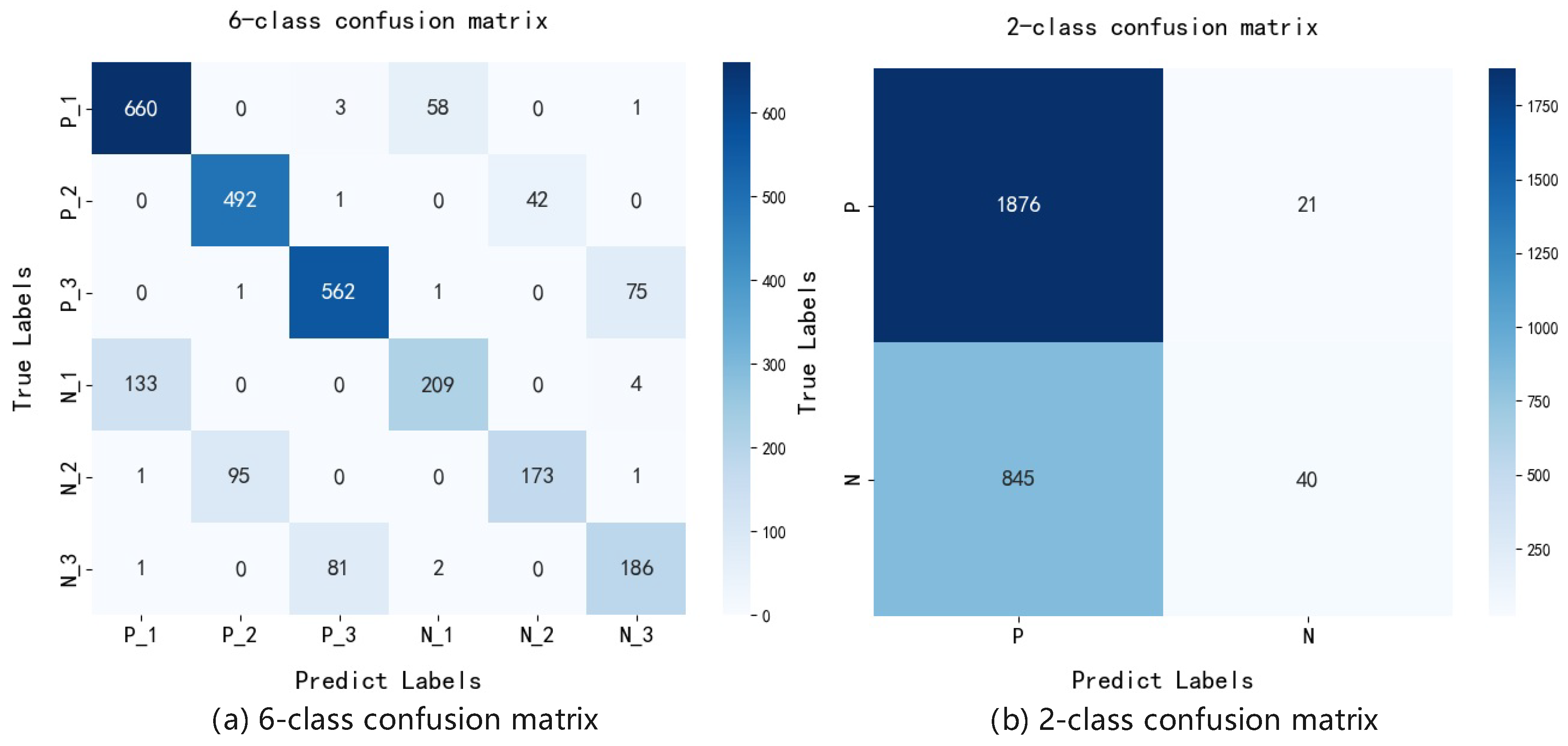
The confusion matrix results for both classification schemes are shown in Figure 9, where the horizontal axis represents the model’s predicted labels, and the vertical axis represents the true labels for normal and abnormal instances across the three actions. In binary classification, the model predominantly classifies all samples as normal, failing to detect abnormal cases, which suggests that the model lacks true decision-making and analytical capabilities under this classification scheme. In contrast, the six-class classification matrix shows that maximum values are concentrated along the diagonal, indicating good overall performance. Further analysis reveals that two-thirds of abnormal samples are correctly detected, aligning with the goal of minimizing missed detections. Additionally, false positives for normal samples remain below 10%, meeting expected performance targets.

Given these findings, this study adopts the STFGCL network with a six-class classification scheme. However, a key challenge in practical applications is the fusion of classification results across the three actions performed by a subject. Since each action produces an independent classification, an effective method is needed to aggregate these results for a final movement disorder assessment. Assuming equal importance for all three actions, three fusion strategies are considered:

• Scheme 1: A subject is classified as having a movement disorder if at least one action is abnormal.
• Scheme 2: A subject is classified as having a movement disorder if at least two actions are abnormal.
• Scheme 3: A subject is classified as having a movement disorder only if all three actions are abnormal.

The experimental results, shown in

Table 8. Comparative experimental results of different fusion schemes on the dataset of motion impairment assessment.

Scheme	Overall Accuracy (%)	False Positive (%)
Scheme 1	80.56	9.83
Scheme 2	73.09	3.26
Scheme 3	61.62	0.75

, indicate that Scheme 1 achieves the highest accuracy of 80.56%, while Scheme 2 and Scheme 3 decrease progressively to 73.09% and 61.62%, respectively. The likely reason is that STFGCL still has a relatively high missed detection rate of around 30% for abnormal samples. As the criteria for global abnormality detection become stricter, overall accuracy decreases. However, since the false positive rate for normal samples remains low (<10%), normal subjects are rarely misclassified, minimizing negative effects on accuracy. Specifically, Schema 1 has a false positive rate of only 9.83%, which is within an acceptable range. Considering that movement disorder assessment requires a low missed detection rate and can tolerate a slight increase in false positives, Scheme 1 is deemed the most suitable for real-world applications.

It is important to note that this study assumes equal weighting for the three actions, but in reality, their contributions to assessment may vary. Future optimization could involve hyperparameter tuning or trainable weight adjustments to refine the fusion strategy further.

6. Conclusions

Research indicates that aging is closely linked to motor function decline and neurodegenerative diseases, leading to an increasing prevalence of movement disorders among the elderly. Current assessment methods, including scale-based evaluations and instrument-based diagnostics, suffer from subjectivity, high cost, and long evaluation times. To address these limitations, this study proposes a rapid and objective assessment method for elderly movement disorders based on skeleton-based action recognition. By extracting keypoints from action videos, the method classifies normal and abnormal movements, enabling standardized analysis.

This study designs a data collection scheme in consultation with medical professionals, selecting three representative movements: walking back and forth, standing up and sitting down, and turning around in place. A detailed preprocessing pipeline converts raw video data into keypoint sequences for training action recognition algorithms. The keypoint extraction process is divided into human object detection and pose estimation, where improvements to YOLOv8 and HRNet enhance accuracy and efficiency. The action recognition module, based on ST-GCN, incorporates dynamic adjacency matrices, multi-scale time window transformations, multimodal fusion, and contrastive learning to improve classification of fine-grained movement variations. In summary, this study presents a novel movement disorder assessment framework tailored for universal screening, early intervention, and treatment, offering a practical and scalable solution for elderly care.

However, this article also encountered many problems that are difficult to overcome with existing conditions and technologies during the research and implementation process. First, the motion obstacle assessment algorithm can be improved. Action recognition can further broaden the field of view, either by optimizing within the framework of graph convolution methods, or by attempting to break away from the framework of graph convolution or changing the input modality to RGB videos and depth maps, so that the model is no longer limited to the information of adjacency matrices. Second, the dataset needs to be more complete. In the future, different shooting angles and durations can be fixed in dataset collection to reduce camera shake and continuously expand the size of the dataset. If necessary, the specified gait movements can be expanded to enrich the diversity of the dataset.