
Improved Maneuver Detection-Based Multiple Hypothesis Bearing-Only Target Tracking Algorithm


Abstract
1. Introduction
- The proposed algorithm introduces the use of a range-parameterized method for dividing the observation range into sub-intervals, each employing Cubature Kalman Filtering (CKF) to address the challenges posed by bearing-only measurements. This innovative step reduces the dependency on linearization and mitigates the nonlinearity of measurement equations, offering an improvement over traditional methods like EKF. The application of CKF in each sub-interval effectively handles the known initial position problem and enhances tracking accuracy by reducing errors in filter performance.
- Maneuver detection is integrated using the innovation sequence, which helps in identifying target maneuvers. When a maneuver is detected, the sub-filter parameters are dynamically reset. This method enhances the robustness of the system by addressing filter divergence issues that arise during maneuvers, which is particularly crucial for tracking targets in complex dynamic environments.
- By incorporating the MHT algorithm, the proposed method excels in addressing the measurement ambiguity problem typical of multi-target tracking scenarios. This hybrid approach improves the robustness of the tracking system in the presence of clutter and measurement noise, ensuring accurate data association even when multiple targets are close together. The use of MHT for simultaneous hypothesis generation and pruning based on measurement likelihood further optimizes the performance of the system, particularly when handling uncertain and incomplete data.
2. Materials and Methods
2.1. Bearing-Only Tracking Modeling
2.1.1. Target Motion Model
2.1.2. Measurement Model and System Observability Analysis
2.2. Multiple Hypothesis Bearing-Only Target Tracking Based on Maneuver Detection
2.2.1. Range-Parameterized Cubature Kalman Filter
- (1)
- Distance interval partitioning
- (2)
- Sub-interval filter weight initialization and update
- (1)
- Compute the cubature points
- (2)
- Calculate state predictions using volume points and covariance predictions :
- (3)
- Calculate the volumetric point :
- (4)
- Calculate the quantile prediction and quantile covariance using volumetric points:
- (5)
- Calculate mutual covariance :
- (6)
- Calculate the Kalman filter gain :
- (7)
- Calculate the state estimates and the state covariance :
2.2.2. Modified Maneuver Detection
| Algorithm 1 Range-Parameterized Cubature Kalman Filter (RPCKF) |
|
|
|
|
2.2.3. Integration of MHT and IMD-RPCKF for Bearing-Only Multi-Target Tracking
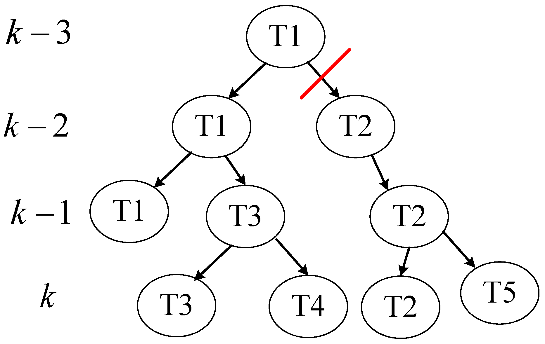
- Hypothesis generation
3. Simulation Results and Analysis
3.1. Simulation Validation of Tracking Performance of the RP-MHTCKF
- (1)
- At PD = 1, the error curves of the Reweighted Pseudo-Nearest Neighbor-based Constrained Kalman Filter (RP-NNCKF) algorithm are similar to those of the RP-JPDACKF algorithm, indicating comparable tracking performance between the two algorithms when no detection omissions occur. The RP-MHTCKF algorithm’s error rapidly decreases at the initial moment, showing overall superior tracking performance compared to the other two algorithms. The RP-MHTCKF algorithm, utilizing the multiple hypothesis framework of the MHT algorithm, initially simulates the target’s position through multiple hypotheses and efficiently eliminates sub-filters generated in incorrect intervals by evaluating the measurement likelihood function and residuals. This process retains only the filters within the correct interval, rapidly minimizing the initial tracking error.
- (2)
- At PD = 0.99, the errors of the RP-JPDACKF and RP-MHTCKF algorithms are similar to those when PD is 1, whereas the RP-NNCKF algorithm is more sensitive to changes in detection probability. When the detection probability is not 1, the error of this algorithm rapidly increases, and the final tracking error never converges. This is because the NN algorithm takes the nearest measurement to the target in relative statistical distance as the true measurement. If the true measurement is missed and no clutter is nearby, the system will take a more distant measurement as the true one, significantly impacting the tracking accuracy of the NN algorithm. In contrast, both of the other algorithms consider detection probability in their state estimation formulas, enhancing system robustness against missed detections. In summary, the RP-MHTCKF algorithm demonstrates superior tracking performance across different simulation scenarios compared to the RP-NNCKF and RP-JPDACKF algorithms.
3.2. Simulation Validation of Tracking Performance of the IMD-MHRPCKF
4. Discussion
5. Conclusions
Author Contributions
Funding
Data Availability Statement
Conflicts of Interest
References
- Sun, N.; Zhao, J.; Shi, Q.; Liu, C.; Liu, P. Moving Target Tracking by Unmanned Aerial Vehicle: A Survey and Taxonomy. IEEE Trans. Ind. Inform. 2024, 20, 7056–7068. [Google Scholar] [CrossRef]
- Wang, K.; Wu, P.; Zhao, B.; Kong, L.; He, S. Reconstructed Variational Bayesian Kalman Filter under Heavy-tailed and Skewed Noises. IEEE Signal Process. Lett. 2024, 31, 2405–2409. [Google Scholar] [CrossRef]
- Wang, K.; Wu, P.; Li, X.; He, S.; Li, J. An adaptive outlier-robust Kalman filter based on sliding window and Pearson type VII distribution modeling. Signal Process. 2024, 216, 109306. [Google Scholar] [CrossRef]
- Wang, K.; Wu, P.; Li, X.; Xie, W.; He, S. A Gaussian–Pearson type VII adaptive mixture distribution-based outlier-robust Kalman filter. Meas. Sci. Technol. 2023, 34, 125160. [Google Scholar] [CrossRef]
- Seme, S.; Štumberger, B.; Hadžiselimović, M.; Sredenšek, K. Solar photovoltaic tracking systems for electricity generation: A review. Energies 2020, 13, 4224. [Google Scholar] [CrossRef]
- Bocus, M.J.; Piechocki, R.J. Passive unsupervised localization and tracking using a multi-static UWB radar network. In Proceedings of the 2021 IEEE Global Communications Conference (GLOBECOM), Madrid, Spain, 7–11 December 2021; pp. 1–6. [Google Scholar]
- Wu, C.; Zhang, F.; Wang, B.; Liu, K.R. mmTrack: Passive multi-person localization using commodity millimeter wave radio. In Proceedings of the IEEE INFOCOM 2020-IEEE Conference on Computer Communications, Toronto, ON, Canada, 6–9 July 2020; pp. 2400–2409. [Google Scholar]
- Li, D.; Du, L. Auv trajectory tracking models and control strategies: A review. J. Mar. Sci. Eng. 2021, 9, 1020. [Google Scholar] [CrossRef]
- Liu, X.; Ren, Z.; Lyu, H.; Jiang, Z.; Ren, P.; Chen, B. Linear and nonlinear regression-based maximum correntropy extended Kalman filtering. IEEE Trans. Syst. Man Cybern. Syst. 2019, 51, 3093–3102. [Google Scholar]
- Liu, C.; Wang, H.; Lin, D.; Cui, X.; Xu, H. Bearings-Only Target Tracking Algorithm with Non-Gaussian Heavy-Tailed Distributed Noise. Acta Armamentarii 2023, 44, 1469. [Google Scholar]
- Hou, L.; Zou, H.; Zheng, K.; Zhang, L.; Zhou, N.; Ren, J.; Shi, D. Orbit estimation for spacecraft based on intermittent measurements: An event-triggered UKF approach. IEEE Trans. Aerosp. Electron. Syst. 2021, 58, 304–317. [Google Scholar] [CrossRef]
- Liu, L.; Mu, R.; Cui, N. A State/Parameter Joint Estimation Algorithm for Active Segment of Multi-stage Ballistic Missile. J. Astronaut. 2023, 44, 1839. [Google Scholar]
- Choe, Y.; Song, J.W.; Park, C.G. Lightweight marginalized particle filtering with enhanced consistency for terrain referenced navigation. IEEE Trans. Aerosp. Electron. Syst. 2021, 58, 2493–2504. [Google Scholar]
- Tian, M.; Chen, Z.; Wang, H.; Liu, L. An intelligent particle filter for infrared dim small target detection and tracking. IEEE Trans. Aerosp. Electron. Syst. 2022, 58, 5318–5333. [Google Scholar]
- Zhang, K.; Wang, H.; Zhang, H.; Luo, N.; Ren, J. Target tracking of UUV based on máximum correntropy high-order UGHF. IEEE Trans. Instrum. Meas. 2023, 72, 8506616. [Google Scholar]
- Wang, S.; Li, H.; Wang, B. Passive Localization Method Based on Range-Parameterised Cubature Kalman Filter. In Proceedings of the 2021 40th Chinese Control Conference (CCC), Shanghai, China, 26–28 July 2021; pp. 280–284. [Google Scholar]
- Lu, Z.; Wenbi, R.; Daxing, X.; Hailun, W. Two-stage high-degree cubature information filter. J. Intell. Fuzzy Syst. 2017, 33, 2823–2835. [Google Scholar]
- Sun, M.; Davies, M.E.; Proudler, I.K.; Hopgood, J.R. Adaptive kernel Kalman filter. IEEE Trans. Signal Process. 2023, 71, 713–726. [Google Scholar]
- Zhang, H.; Liu, W.; Zong, B.; Shi, J.; Xie, J. An efficient power allocation strategy for maneuvering target tracking in cognitive MIMO radar. IEEE Trans. Signal Process. 2021, 69, 1591–1602. [Google Scholar]
- Singer, R.; Sea, R. New results in optimizing surveillance system tracking and data correlation performance in dense multitarget environments. IEEE Trans. Autom. Control 1973, 18, 571–582. [Google Scholar]
- Zhang, X.; Wu, N.; Wang, F.; Tong, L. Skip-glide target tracking based on improved Jerk model. Command. Control Simul. 2023, 45, 62–69. [Google Scholar]
- Zeng, H.; Mu, W.; Jiang, Y.; Yang, S. Model Parameter Adaptive Low-Complexity ATPM-VSIMM Algorithm. J. Commun. 2023, 44, 25–35. [Google Scholar]
- Feng, H.; He, Y.; Xu, H.; Wang, X. Fuzzy Inference Based STPF-AIMM Surface Target Tracking Algorithm. J. Huazhong Univ. Sci. Technol. (Nat. Sci. Ed.) 2023, 51, 109–114. [Google Scholar]
- Chen, Y.; Liu, Q.; Li, L.; Kang, L. A New Method for Maneuvering Target Tracking Based on Minimum Fuzzy Error Entropy. Acta Electron. Sin. 2023, 51, 2408–2418. [Google Scholar]
- Shen, L.; Su, H.; Li, Z.; Jia, C.; Yang, R. Self-attention-based Transformer for nonlinear maneuvering target tracking. IEEE Trans. Geosci. Remote Sens. 2023, 61, 1–13. [Google Scholar] [CrossRef]
- Yun, P.; Wu, P.; Li, X.; He, S. Variational Bayesian Probability Data Association Algorithm. Acta Autom. Sin. 2022, 48, 2486–2495. [Google Scholar]
- Li, X. Research on Underwater Multi-Target Tracking Technology Based on Information Fusion. Ph.D. Thesis, Northwestern Polytechnical University, Shaanxi, China, 2016. [Google Scholar]
- Kumar, M.; Mondal, S. Recent developments on target tracking problems: A review. Ocean Eng. 2021, 236, 109558. [Google Scholar] [CrossRef]
- Zhu, Y.; Mallick, M.; Liang, S.; Yan, J. Generalized labeled multi-Bernoulli multi-target tracking with Doppler-only measurements. Remote Sens. 2022, 14, 3131. [Google Scholar] [CrossRef]
- Sheng, T.; Xia, H.; Yang, Y. Simplified JPDA Multi-Target Tracking Algorithm in Dense Clutter Environment. Signal Process. 2020, 36, 1280–1287. [Google Scholar]
- Li, X.; Wang, Z.; Zhang, Y.; Lu, X. Improved MHT Algorithm Based on Adaptive GMM Clutter Estimation. J. Terahertz Sci. Electron. Inf. Technol. 2023, 21, 794–800. [Google Scholar]
- Han, W.; Wang, G.; Yan, K.; Song, Y. Doppler Blind Zone Target Plot-Track Association Method Based on Multidimensional Allocation. Syst. Eng. Electron. 2023, 45, 3091–3097. [Google Scholar]


| Time/s | Motion Model | Radial Velocity |
|---|---|---|
| 1–10 | Uniform accelerated motion | Acceleration (0.8 m/s2, −0.8 m/s2) |
| 10–25 | Uniform turning motion | Angular velocity rad/s |
| 25–100 | Uniform linear motion | Velocity (−8 m/s, 8 m/s) |
| Time (s) | Motion Model | Motion Parameters |
|---|---|---|
| 1–10 | Constant acceleration motion | Acceleration (0.8 m/s2,−0.8 m/s2) |
| 10–25 | Constant turn motion | Angular velocity ( rad/s) |
| 25–80 | Constant velocity linear motion | Velocity (−8 m/s, −8 m/s) |
| 80–95 | Constant turn motion | Angular velocity ( rad/s) |
| 95–150 | Constant velocity linear motion | Velocity (8 m/s, −8 m/s) |
| Algorithm | IMD- MHRPCKF | MD- CPHDRPCKF | MD- JDPARCKF | MD- NNRPCKF |
|---|---|---|---|---|
| OSPA (m) | 58.10 | 81.67 | 132.23 | 554.69 |
Disclaimer/Publisher’s Note: The statements, opinions and data contained in all publications are solely those of the individual author(s) and contributor(s) and not of MDPI and/or the editor(s). MDPI and/or the editor(s) disclaim responsibility for any injury to people or property resulting from any ideas, methods, instructions or products referred to in the content. |
© 2025 by the authors. Licensee MDPI, Basel, Switzerland. This article is an open access article distributed under the terms and conditions of the Creative Commons Attribution (CC BY) license (https://creativecommons.org/licenses/by/4.0/).
Share and Cite
Liu, X.; Wu, P.; Bo, Y.; Liu, C.; Hu, H.; He, S. Improved Maneuver Detection-Based Multiple Hypothesis Bearing-Only Target Tracking Algorithm. Electronics 2025, 14, 1439. https://doi.org/10.3390/electronics14071439
Liu X, Wu P, Bo Y, Liu C, Hu H, He S. Improved Maneuver Detection-Based Multiple Hypothesis Bearing-Only Target Tracking Algorithm. Electronics. 2025; 14(7):1439. https://doi.org/10.3390/electronics14071439
Chicago/Turabian StyleLiu, Xinan, Panlong Wu, Yuming Bo, Chunhao Liu, Haitao Hu, and Shan He. 2025. "Improved Maneuver Detection-Based Multiple Hypothesis Bearing-Only Target Tracking Algorithm" Electronics 14, no. 7: 1439. https://doi.org/10.3390/electronics14071439
APA StyleLiu, X., Wu, P., Bo, Y., Liu, C., Hu, H., & He, S. (2025). Improved Maneuver Detection-Based Multiple Hypothesis Bearing-Only Target Tracking Algorithm. Electronics, 14(7), 1439. https://doi.org/10.3390/electronics14071439