Traffic-Forecasting Model with Spatio-Temporal Kernel

Abstract

Within the realm of intelligent transportation systems, the precise forecasting of vehicular speed across individual road segments constitutes a fundamental task. This metric serves as a pivotal indicator for evaluating the extent of network congestion and facilitating informed strategic planning. Contemporary methodologies predominantly employ recurrent neural networks (RNNs) to model temporal dependencies, while leveraging graph convolutional networks (GCNs) to capture spatial dependencies within the data. However, these methods fail to integrate temporal and spatial dependencies to establish global dependencies. This study introduces the spatio-temporal kernel graph convolutional network (STK-GCN), a novel framework designed for modeling and forecasting traffic data. Specifically, we devise a spatio-temporal kernel capable of generating both spatial and temporal matrices, which are subsequently utilized within a encoder–decoder architecture to concurrently capture spatio-temporal dependencies. Furthermore, we introduce a novel temporal graph convolution module to enhance temporal data. To demonstrate the efficacy of the proposed STK-GCN, comprehensive experiments were carried out on two real-world traffic datasets, namely METR-LA and PEMS-BAY. The results indicate that our model surpasses existing state-of-the-art methods.

1. Introduction

Numerous real-world datasets can be represented as structured spatio-temporal sequences, encompassing domains such as traffic management [1] and climate science [2], among others. In the context of traffic-management applications, sensors are strategically deployed at diverse locations along roadways to collect pertinent data at each temporal interval across various regions, including metrics such as traffic volume and vehicular velocity. Traffic forecasting constitutes a pivotal task within intelligent transportation systems (ITS) [3]. Accurate prediction of traffic conditions across various regions enables administrators to devise more effective traffic-management strategies, preemptively mitigate potential risks, and improve the overall transportation efficiency of the area.

The problem of traffic prediction presents significant challenges, not only due to complex temporal dependencies but also because of intricate spatial dependencies [4]. Most early methods only concentrated on capturing temporal dependencies but ignored the spatial correlations. These methods include statistical approaches such as autoregressive integrated moving average (ARIMA) [5] and shallow machine-learning methods like support vector regression (SVR) [6]. These traditional algorithms have achieved acceptable prediction accuracy in small-scale traffic-flow forecasting tasks. Subsequent studies, including diffusion convolutional recurrent neural network (DCRNN) [7] and spatio-temporal graph convolutional networks (STGCN) [8], identified the constraints inherent in the previously mentioned approaches and incorporated graph convolutional networks (GCN) to model spatial dependencies within traffic data. In DCRNN, recurrent neural networks (RNNs) are utilized to capture temporal dynamics, thereby enhancing the long-term dependency modeling capability of spatio-temporal graph neural networks. STGCN, on the other hand, introduced a comprehensive deep-learning framework utilizing a fully convolutional architecture for traffic forecasting, which enhances training efficiency and minimizes the parameter count. Next, there are many related works based on graph neural networks (GNNs), such as graph convolutional recurrent network (GCRN) [9], spectral temporal graph neural network (StemGNN) [10], residual recurrent graph neural network (Res-RGNN) [11], spatio-temporal graph convolutional neural network (GCNN) [12], and so on.

All of these works share a common characteristic, which is the requirement of a geographically informed adjacency matrix as input for graph convolution. However, this adjacency matrix is inadequate for capturing the intricate spatiotemporal dependencies inherent in traffic data. Scholars aim to GNN networks that do not rely on geographic graph inputs. A notable contribution in this domain is the Graph WaveNet (GWNet) [13], which captures latent spatial dependencies by incorporating an adaptive dependency matrix derived from node embedding techniques. Networks including graph time series (GTS) [14] and multivariate time-series graph neural network (MTGNN) [15] develop this viewpoint and improve the adaptive graph from their respective perspectives. These geography-independent approaches have demonstrated considerable efficacy in traffic-forecasting tasks, garnering growing interest within the research community. However, despite the notable advancements achieved by these GNN-based methodologies, two critical challenges remain unresolved. (1) Existing models are limited in their capacity to effectively capture and manage the latent dependencies that exist across diverse spatio-temporal contexts. These dependencies, which are often complex and dynamic, are crucial for accurate traffic forecasting but remain inadequately addressed by current methodologies. (2) Adaptive graph-based models, while innovative, exhibit a lack of stability in their performance. This instability can be attributed to the variability in the learned graph structures, which may lead to inconsistent predictions and hinder the reliability of the model in practical applications.

To handle the above two key challenges, we introduce a novel spatio-temporal kernel graph convolutional network (STK-GCN) framework designed for traffic forecasting. Inspired by the idea of adaptive graph, we have devised a spatio-temporal kernel that is utilized not only for generating spatially adaptive graphs but also for concurrently producing temporally adaptive graphs. Since adaptive graphs do not require predefined graph inputs, we have introduced temporal adaptive graph convolutions, utilizing the temporally adaptive graphs generated by the spatio-temporal kernel as the input graphs for the convolution operations. The primary contributions of this study are outlined as follows:

• We introduce an innovative spatio-temporal kernel designed for graph learning, which explicitly disentangles spatial and temporal heterogeneity. To the best of our knowledge, this represents the first instance of employing a spatio-temporal kernel to concurrently generate both spatial and temporal graph matrices.
• We introduces the temporal graph convolution module to enhance temporal feature representation.
• The model was evaluated on two real-world datasets, demonstrating superior performance relative to a suite of state-of-the-art models.

2. Related Works

Traffic forecasting has been a subject of extensive research over the years, driven by the increasing complexity of urban transportation networks and the need for efficient traffic-management systems. Earlier, researchers studied this issue using traditional statistical methods, such as ARIMA and vector autoregression (VAR) [16]. These approaches are limited to modeling linear temporal relationships and entirely overlook the incorporation of spatial dependencies. Subsequently, various shallow machine-learning techniques, such as support vector regression (SVR) [6] and k-nearest neighbors (KNN) [17], were employed for traffic-prediction tasks. These methods share common drawbacks of requiring manual feature extraction and having limited generalization capabilities, typical of shallow machine-learning approaches. With the evolution of deep learning and the enhancement of computational capabilities, researchers have increasingly adopted deep-learning methodologies for traffic prediction. A notable method was the RNN [18]. Later, variants of RNNs such as LSTM [19] and GRU [20] have shown promising performance in traffic prediction.

Transformers [21], originally introduced from the field of computer vision, have also been applied to solve time-series prediction problems. Lastjomer [22] learned a spatio-temporal joint attention to capture the dynamic dependencies. LogSparse Transformer [23] proposed an attention method with low space complexity. In ASTGCN [24], the attention mechanism is used to enhance the attention among present, daily, and weekly timelines. Additional transformer-based models [23,25] have been introduced to address the challenges associated with long-sequence time-series forecasting. However, the attention mechanism also has its limitations. Adding the attention mechanism caused the model to lose its comprehensiveness because traffic problems can occur non-cyclically.

GNNs [26,27] emerged in deep learning to handle graph-structured data, which can model the spatial dependencies within non-Euclidean structures through message-passing mechanisms between nodes. A number of specialized models were recently developed, e.g., GCRN [9], DCRNN [7], MTGNN [15], and StemGNN [10]. These models combine graph convolution and recurrent time units to enhance the feature representation of spatio-temporal data.

Geography-independent graph neural networks (GNNs) do not depend on road network graphs based on geographic information or pre-defined graphs constructed using Euclidean distance. GW-Net [13] pioneered the approach of employing two trainable embedding matrices to generate an adaptive graph directly from the input traffic data. MTGNN [15] and GTS [14] learned a discrete graph structure, while MegaCRN [28] augmented the graph structure learning with a memory network. StemGNN [10] proposed the self-attention learned from the input as the graph. HOMGNN [29] combined the geography-dependent graph and self-learning graph to extract higher-order spatial dependencies. Our work distinguishes itself from these methods by generating a time graph and space graph simultaneously through a shared kernel.

In the context of traffic prediction, it is important to note that some authors regard artificial neural networks (ANN) and machine-learning models as a “black box” [30,31,32]. This is because these models do not provide an explicit or interpretable relationship between the independent variables (e.g., traffic data, spatial-temporal features) and the dependent variable (e.g., traffic speed or volume). Instead, they rely on complex, non-linear transformations that are often difficult to translate into a clear, transferable equation. As a result, while these models can achieve high predictive accuracy, their lack of transparency limits their interpretability and practical applicability in scenarios where understanding the underlying mechanisms is crucial. This characteristic underscores the trade-off between model performance and interpretability in traffic-forecasting research.

3. Method

3.1. Problem Definition

In the traffic-forecasting task, traffic speed is recorded using loop detectors installed on roadways. These detectors measure the speed of vehicles passing over them at time intervals. For each interval, the average speed of all vehicles detected during that time window is calculated and recorded. The data are stored as a time series for each sensor, reflecting the temporal variations in traffic speed. We receive signals from m moments $[X_{t-m},\dots ,X_t]$, and based on this, we need to predict the results at the next n moments $[X_{t+1},\dots ,X_{t+n}]$, where $X_i\in {\mathbb{R}}^{N\times C}$, N represents the total number of sensors deployed across the traffic network, while C denotes the number of input channels. So, essentially, the objective of the traffic-forecasting task is to learn a mapping function $F(·)$ that predicts the future n time steps of signals $Y\in {\mathbb{R}}^{n\times N\times C}$ based on the observed m time steps of signals $X\in {\mathbb{R}}^{m\times N\times C}$, parameterized by $\theta$.

$$[X_{t-m},\dots ,X_t]\underset{\theta }{\stackrel{F(·)}{⟶}}[X_{t+1},\dots ,X_{t+n}]$$

(1)

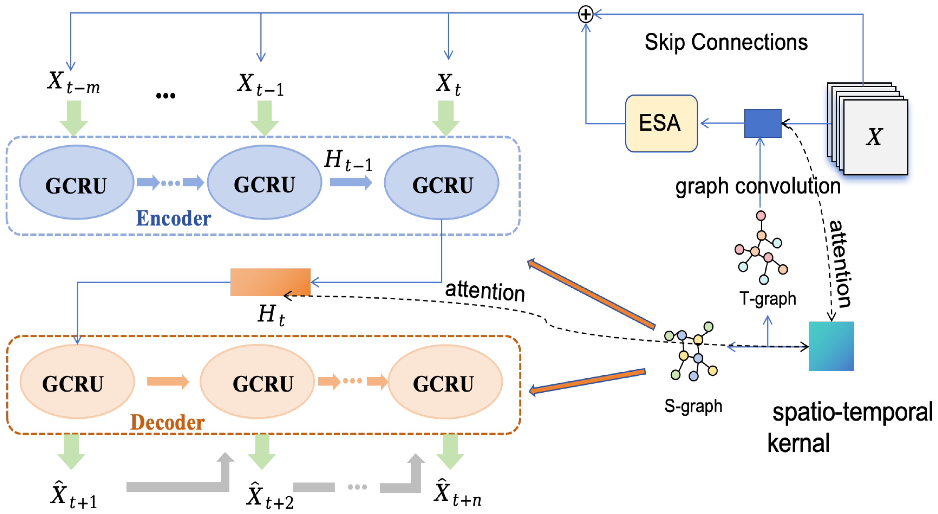
3.2. Model Architecture

This section provides a comprehensive description of our methodology. Figure 1 depicts the architecture of the proposed STK-GCN, which consists of an encoder, a decoder, a temporal graph convolution module, and a spatio-temporal kernel. Both the encoder and decoder share an identical architecture, integrating gated recurrent units (GRUs) with graph neural networks (GNNs) to effectively model spatial dependencies. In addition to employing spatial graph convolution in the GRU, we have also introduced a novel temporal graph convolution. Both types of graph convolution require a graph as input, and both graphs are generated by our spatio-temporal kernel. The spatio-temporal kernel generates both the T-graph and the G-graph without the need for predefined graphs as input. Throughout the model, the traffic data X serves as the raw data input, which is fed into the encoder after undergoing temporal graph convolution module, and finally, the decoder outputs the predicted values for the specified number of future steps.

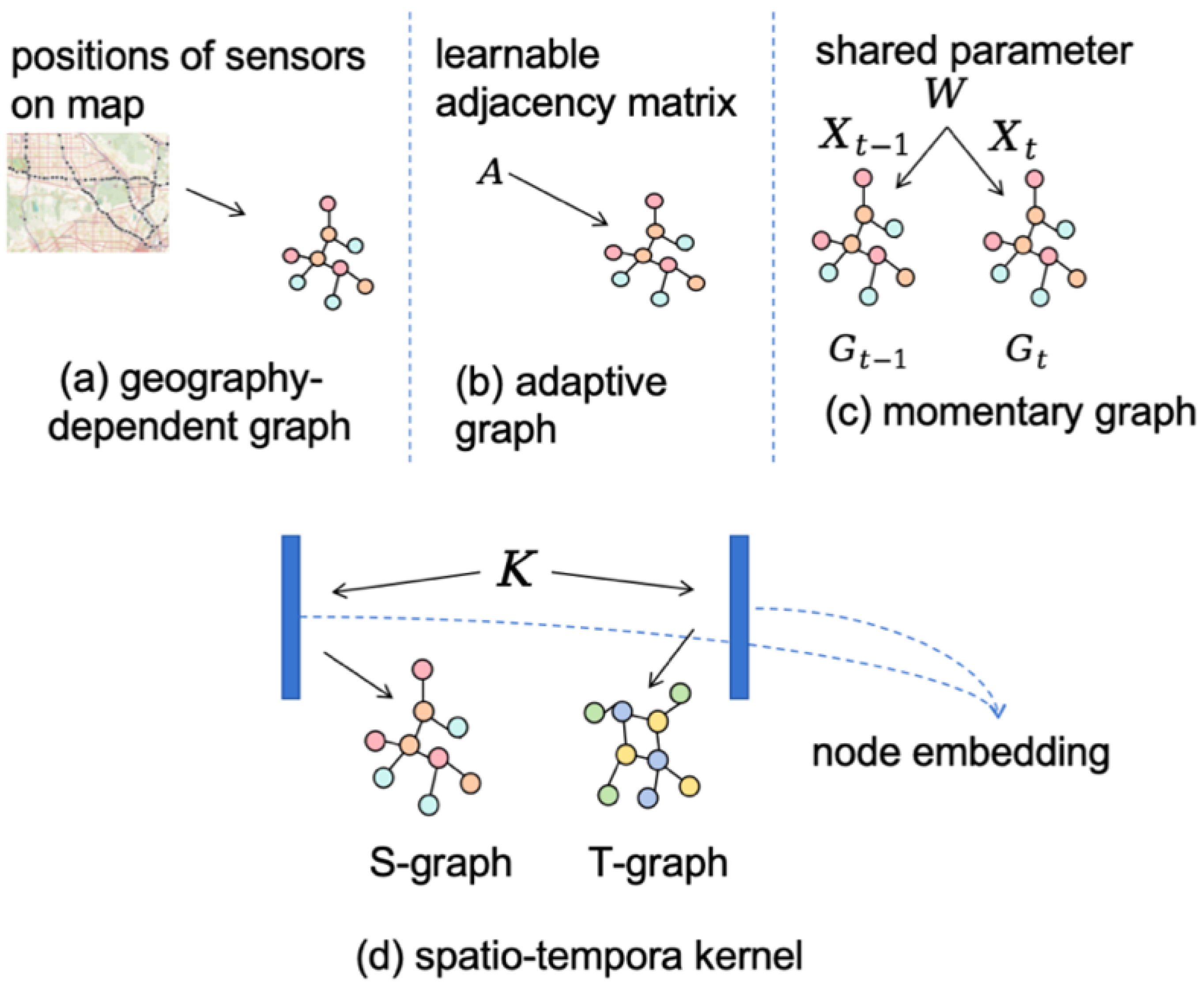
3.2.1. Spatio-Temporal Kernel

In this section, we formally introduce a novel graph-learning module termed the spatio-temporal kernel. In the graph convolution process, we require an input graph. Many methods typically use graph based on topology structure or empirical laws as inputs. However, this prior information does not reflect latent dependencies.

We aim to enhance spatio-temporal dynamic extraction, specifically targeting the relational dependencies among contextual timestamps. Therefore, we propose the spatio-temporal kernel to learn the latent spatio-temporal graph. Specifically, the kernel is a two-dimensional matrix, and we use linear transformations to generate embeddings for both spatial and temporal dimensions separately. Then the embeddings are used to generate matrices. Figure 2 shows the development of the adaptive graph. Figure 2a is the geography-dependent graph, which utilizes the real world map to to construct graph structures, Figure 2b is the adaptive graph, using a learnable matrix to to replace the adjacency matrix, Figure 2c uses parameter sharing and updates the adaptive graph at each time step, and Figure 2d is our spatio-temporal kernel, which first generates point embeddings for time and space separately through a kernel, and then uses these point embeddings to generate time graph and space graph.The mathematical formulations of which are illustrated as follows:

$$E_{s1}=W_{s1}·K$$

(2)

$$E_{s2}=W_{s2}·K$$

(3)

$${\mathcal{G}}_s=tanh\left(relu(E_{s1}·E_{s2}^T)\right)$$

(4)

$$E_{t1}=W_{t1}·K$$

(5)

$$E_{t2}=W_{t2}·K$$

(6)

$${\mathcal{G}}_t=tanh\left(relu(E_{t1}·E_{t2}^T)\right)$$

(7)

where $E_{s1}$ and $E_{s2}$ represent two randomly initialized spatial graph embedding matrices, while $E_{t1}$ and $E_{t2}$ denote temporal embeddings. ${\mathcal{G}}_s$ and ${\mathcal{G}}_t$ are adjacency matrices generated by spatio-temporal kernel.

Two distinct types of graph convolutions are applied to the initial input data X. $X\in {\mathbb{R}}^{m\times N\times C}$ is the original input data, where m represents the number of initial input time steps Equation (1). The temporal graph convolution is performed along the first dimension m, while the spatial graph convolution is performed along the second dimension N. This implies that the temporal graph matrix has a dimensionality of $m\ast m$, while the spatial graph convolution matrix possesses a dimensionality of $N\ast N$. The two graph matrices are used separately for temporal graph convolution and spatial graph convolution. These two modules will be detailed in the following sections.

Following the graph convolution operation, an attention mechanism is incorporated to refine and update the spatio-temporal kernel. The resultant features are multiplied by the spatio-temporal kernel, and a softmax function is subsequently applied to derive similarity scores. These similarity scores are then multiplied by the spatio-temporal kernel to obtain the final feature output.

$$Q=\left(X_{\ast \mathcal{G}}\right)·W_Q+b_Q$$

(8)

$$S=\mathrm{softmax}(Q·K^T)$$

(9)

$$X^{\ast }=S·K$$

(10)

where $X_{\ast \mathcal{G}}$ represents graph convolution with $\mathcal{G}$ as the graph input, and W and K represent trainable weight parameters. $X^{\ast }$ represents the output features after the dot-product attention. For convenience, we express this dot-product attention as $Attention(·,K)\in {\mathbb{R}}^{m\times N\times C}\mapsto {\mathbb{R}}^{m\times N\times C}$.

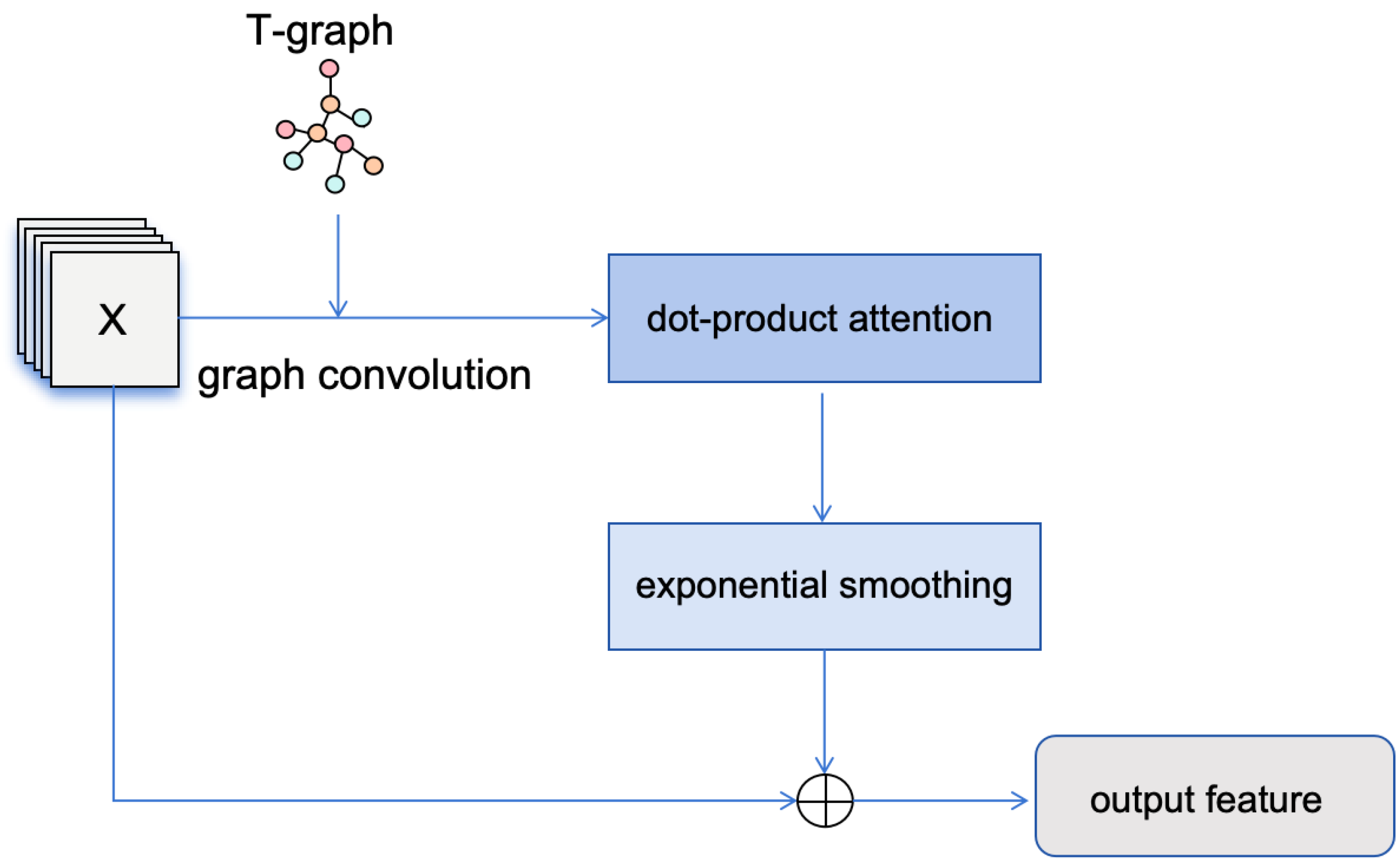
3.2.2. Temporal Graph Convolution Module

Time flows in one direction, and thus researchers’ studies on time series focus on inferring the future from the past. However, temporal features can also exhibit non-one-dimensional structures. Given the significant efficacy of adaptive graphs in modeling spatial relationship dependencies, this section aims to extend their utility to the extraction of temporal dynamics, specifically the relationship dependencies between successive time steps. The challenge in applying graph convolution to capture temporal dynamics lies in the lack of explicit associations between consecutive time steps, meaning there is no explicit temporal graph.

To tackle this challenge, this section introduces a temporal graph convolution module, comprising two distinct components. The first component is the graph convolution, and the second component is the exponential smoothing method. These two components are connected sequentially and, in conjunction with residual connections, constitute the temporal graph convolution module. The architecture of the temporal graph convolution module is depicted in Figure 3. The specific expression is as follows:

$$\begin{array}{c}\hfill X_{\ast {\mathcal{G}}_t}=[\mathrm{dropout}\left(\mathrm{relu}(X{W}_1{\mathcal{G}}_t+b_1)W_2{\mathcal{G}}_t\right)+b_2]\end{array}$$

(11)

where ${\mathcal{G}}_t$ represents the temporal graph, while W and b are the learnable parameters in the linear transformation. $X\in {\mathbb{R}}^{m\times N\times C}$ represents the original input data, where m represents the number of initial input time steps Equation (1), N represents the number of sensors in the map, and C represents the number of channels in the input data. During the convolution process, dropout is employed to improve the generalization capability of the temporal graph convolution module. Following the graph convolution operation, the resultant features are passed into the dot-product attention module, as illustrated in Equations (8)–(10).

The second part is inspired by Holt–Winters’ exponential smoothing method [33], which assume that time-series can be decomposed into seasonal and trend components, and trend can be further decomposed into level and growth components. The method can be formulated as follow:

$$L_t=\alpha ·X_t+(1-\alpha )·(L_{t-1}+T_{t-1})$$

(12)

$$T_t=\beta ·(L_t-L_{t-1})+(1-\beta )·T_{t-1}$$

(13)

$$S_t=\gamma ·(Y_t-L_t)+(1-\gamma )·S_{t-m}$$

(14)

$${\widehat{X}}_{t+h}=L_t+h{T}_t+S_{t+h-m}$$

(15)

In these equations, $L_t$ denotes the estimated level at time t, $T_t$ represents the trend estimate, $S_t$ represents the seasonality estimate, $Y_t$ is the observed value, and $\alpha$, $\beta$, and $\gamma$ represent the smoothing parameters corresponding to level, trend, and seasonality, respectively. m represents the length of the seasonal cycle. The final equation is the prediction after h time steps. Based on the above expression, it can be seen that the core idea of this method is the exponential decay from the previous temporal feature, and the decay weight is controlled by $\alpha$, $\beta$, and $\gamma$.

Inspired by the Holt–Winters method [33], our goal is to give higher weight to recently observed data. This is an innovative form of attention, where the weights are calculated based more on relative time stamps. The smoothing process can be characterized by the following expression:

$$\begin{array}{c}\hfill \mathcal{E}{\left(X\right)}_t=\alpha X_t+(1-\alpha )\mathcal{E}{\left(X\right)}_{t-1}\end{array}$$

(16)

where $\mathcal{E}(·)\in {\mathbb{R}}^{m\times N\times C}\mapsto {\mathbb{R}}^{m\times N\times C}$ means the exponential smoothing operation on the given sequence X with length m, $\alpha$ is a learnable parameter, and the subscript t corresponds to the t-th row of the output. Note that the input X here is the output from the dot-product attention module.

The integration of a temporal graph convolution and exponential smoothing module provides an efficient and powerful analytical tool for processing temporal graph data. Temporal graph convolution captures temporal dependencies among nodes in graph structures, extracting features along the time dimension through convolutional operations, thereby revealing dynamic patterns and trends in time-series data. However, when dealing with highly volatile or noisy data, temporal graph convolution may be affected by outliers or short-term fluctuations, leading to instability in capturing long-term trends.

The introduction of the exponential smoothing module effectively addresses this limitation. Exponential smoothing applies a weighted average to historical data, assigning higher weights to more recent data, thereby preserving the main trends of the time series while smoothing out short-term fluctuations and noise. This characteristic enables the exponential smoothing module to provide more stable and reliable input for temporal graph convolution, enhancing the model’s ability to model long-term temporal dependencies. Additionally, the recursive computation of exponential smoothing ensures high computational efficiency, allowing seamless integration with the efficient computational framework of temporal graph convolution.

In summary, the integration of temporal graph convolution and exponential smoothing module not only enhances the model’s feature extraction capability for time-series data but also improves its stability and generalization performance. This combination provides a robust theoretical framework for the analysis of traffic prediction.

3.2.3. Graph Convolutional Recurrent Unit

Drawing inspiration from the achievements of RNNs in the domains of natural language processing (NLP) and computer vision (CV), a series of studies have commenced applying RNNs to spatio-temporal data. Recent research has investigated the potential of integrating graph convolution operations within recurrent cells, such as LSTM. After incorporating graph neural networks, RNN networks are capable of concurrently capturing temporal and spatial features. We employ gated recurrent units (GRU) to model temporal dependencies, a robust variant of recurrent neural networks (RNNs). In DCRNN [7], the conventional linear operations within the GRU are substituted with a diffusion graph convolution network. Our work distinguishes itself from this by introducing the concept of partial convolution GRU, which reduced the number of parameters and improved training efficiency. Typically, a GRU comprises an update gate and a reset gate to regulate the flow of information. We propose a novel concept of partial convolution GRU, which only applies graph convolution to the state in the reset gate. The specific expressions are as follows:

$$U_t=\sigma ([X_t,H_{t-1}]·W_u+b_u)$$

(17)

$$R_t=\sigma ([X_t,H_{t-1}]·W_r+b_r)$$

(18)

$$C_t=tanh({[X_t,H_{t-1}]}_{\ast {\mathcal{G}}_s}·W_c+b_c)$$

(19)

$$H_t=U_t·H_{t-1}+(1-U_t)·C_t$$

(20)

where $X_t\in {\mathbb{R}}^{m\times N\times C}$ represents the input to the graph convolution unit at time step t. $H_t\in {\mathbb{R}}^{m\times N\times h}$ denotes the output of graph convolution operation, where h is the hidden dimension. $W_u,W_r\in {\mathbb{R}}^{(C+h)\times h}$ are the weight matrices and $b_u,b_r\in {\mathbb{R}}^h$ are biases. $\ast {\mathcal{G}}_s$ represents the data that undergoes the graph convolution operation with graph ${\mathcal{G}}_s$.

Distinguished from Equation (11) for temporal graph convolution, we adopt the classical definition of graph convolution to capture spatial dependencies, which requires an adjacency matrix as input for the graph and applies this matrix to a kth-order Chebyshev polynomial [34]. This method approximates the graph Laplacian eigenvalues using Chebyshev polynomials to perform efficient convolution operations. This approach is primarily used for large-scale graph data as it captures local features of the graph structure while maintaining model efficiency. However, we utilize an adaptive graph in place of a pre-defined graph structure. Consequently, we substituted the eigenvalue matrix of the normalized graph Laplacian matrix in the original formulation with an adaptive matrix.

$$\begin{array}{c}\hfill X_{\ast {\mathcal{G}}_s}=\sigma \left(\sum _{k=0}^{K-1}{\tilde{T}}_k\left({\mathcal{G}}_s\right)X{\mathsf{\Theta }}_k\right)\end{array}$$

(21)

where X is the input, $\mathcal{G}$ is the adaptive matrix learned from our spatio-temporal kernel, and ${\tilde{T}}_k(·)$ denotes the normalized k-th order Chebyshev polynomial.

3.2.4. Encoder Stacks and Decoder Stacks

Before feeding the data into the encoder, we process $X\in {\mathbb{R}}^{m\times N\times C}$ through our temporal graph convolution module to enrich the temporal representation, yielding $X_{\ast {\mathcal{G}}_t}\in {\mathbb{R}}^{m\times N\times C}$. Afterward, we input the graph convolution processed data into our attention module and exponential smoothing module to obtain the reconstructed representation $X^{\prime }\in {\mathbb{R}}^{m\times N\times C}$. The appeal process is reflected in Equation (22). The encoding layers utilize the GCRU units mentioned above, which takes input data $[X_{t-i-1}^{\prime },X_{t-i-1}]$ and the state $H_t$ from the previous unit. t represents the data at the t-th timestamp in sequence X. The overall equations for encoder layer can be formulated as:

$$X^{\prime }=\mathcal{E}\left(Attention(X_{\ast {\mathcal{G}}_t},K)\right)$$

(22)

$$H_{t-i}=\mathrm{GCRU}([X_{t-i-1}^{\prime },X_{t-i-1}],H_{t-i-1})(i=1,\dots ,m-1)$$

(23)

$$H_t=Attention(\mathrm{GCRU}([X_{t-1}^{\prime },X_{t-1}],H_{t-1}),K)$$

(24)

where $\ast {\mathcal{G}}_t$ denotes the graph convolutional with graph $\ast {\mathcal{G}}_t$, $\mathcal{E}$ denotes the exponential smoothing, and GCRU represents our graph convolutional recurrent unit. $Attention(·,K)$ means the dot-product attention in Equations (8)–(10) with the spatio-temporal kernel K.

Similar to the encoder, each GCRU unit in the decoder takes the input data $X_{i-1}$ and the state $H_{i-1}$ to produce the prediction ${\widehat{X}}_i$ and hidden state $H_i$. We set the initial input as a tensor filled with zeros, and the initial state comes from the encoder. Unlike the encoder, the output of the decoder is fed through a fully connected layer to generate predictions, which subsequently serve as the input for the next GCRU unit. Utilizing the hidden states $H_t$ obtained from the encoder, the decoder’s operations can be summarized by the following equations:

$$\begin{array}{cc}\hfill {\widehat{X}}_{t+h},H_{t+h}& =\mathrm{GCRU}({\widehat{X}}_{t+h-1},H_{t+h-1})\hfill \end{array}$$

(25)

With the architecture described, we present the proposed spatio-temporal kernel graph convolutional network (STK-GCN) as a generic framework for traffic forecasting.

4. Experiments

4.1. Datasets

We trained our model on two large-scale traffic datasets, PEMS-BAY and METR-LA. The METR-LA and PEMS-BAY datasets capture traffic-speed data from two major metropolitan regions in California, USA. The METR-LA dataset covers Los Angeles County, including highways like I-5 and US-101, with data from 207 sensors. The PEMS-BAY dataset spans the San Francisco Bay Area, covering routes such as I-280 and I-880, with data from 325 sensors. Figure 4 illustrates the locations of sensors on the map. In both datasets, the traffic-speed data are normalized using Z-score standardization. Each dataset is split into training set, validation set, and test set with a ratio of 7:1:2, following the traditional work.

Table 1. Information of METR-LA and PEMS-BAY.

Dateset	Nodes	Start Time	Timesteps
METR-LA	207	1 March 2012	34,272
PEMS-BAY	325	1 January 2017	52,116

presents the information of the two datasets.

4.2. Parameter Settings and Evaluation Metrics

Both the observation step m and the prediction horizon n are configured to 12, indicating that the model utilizes historical data from the preceding hour to forecast traffic conditions for the subsequent hour, consistent with established practices in prior research [7,8]. All traffic-speed data have been standardized using z-score normalization $z=(x-u)/\sigma$, where x denotes traffic speed, u denotes average speed of training set, and $\sigma$ denotes the standard deviation of training set. The Adam optimizer was employed, with an initial learning rate of 0.01, which was reduced by a factor of 0.1 at the 45th and 75th epochs. The batch size was configured to 64. Three widely-used metrics, mean absolute error (MAE), root mean squared error (RMSE), and mean absolute percentage error (MAPE), were utilized to assess the prediction performance. These metrics are formulated as follows:

$$\begin{array}{c}\hfill MAE={\displaystyle \frac{1}{nT}}\sum _{t=1}^T\sum _{i=1}^n|X_{t+i}-{\widehat{X}}_{t+i}|\end{array}$$

(26)

$$\begin{array}{c}\hfill RMSE=\sqrt{{\displaystyle \frac{1}{nT}}\sum _{t=1}^T\sum _{i=1}^n{(X_{t+i}-{\widehat{X}}_{t+i})}^2}\end{array}$$

(27)

$$\begin{array}{c}\hfill MAPE={\displaystyle \frac{100}{nT}}\sum _{t=1}^T\sum _{i=1}^n\left|{\displaystyle \frac{X_{t+i}-{\widehat{X}}_{t+i}}{X_{t+i}}}\right|\end{array}$$

(28)

where T denotes the total number of time steps in the series, and n represents the horizon of a single time series. MAE is also used as loss function:

$$\begin{array}{c}\hfill L\left(\mathsf{\Theta }\right)={\displaystyle \frac{1}{nT}}\sum _{t=1}^T\sum _{i=1}^n|X_{t+i}-{\widehat{X}}_{t+i}|\end{array}$$

(29)

where $\mathsf{\Theta }$ represents the complete set of parameters within our model.

4.3. Baselines

We evaluate the performance of our STK-GCN against several widely recognized traffic-forecasting models, including STGCN, DCRNN, and GWNet, among others.

• Spatio-temporal graph convolutional networks (STGCN) [8]. A generic graph-based formulation for modeling dynamic skeletons, which is the first that applies graph-based neural networks for this task.
• Diffusion convolutional recurrent neural network (DCRNN) [7]. DCRNN employs an encoder–decoder framework for multi-step forecasting and substitutes the linear operations within the gated recurrent unit (GRU) with a diffusion graph convolution network.
• Graph WaveNet (GWNet) [13]. An advanced model derived from STGCN, which pioneers the use of an adaptive adjacency matrix to model spatial dependencies.
• Multivariate time-series graph neural network (MTGNN) [15]. An enhanced variant of GWNet, which eliminates the reliance on any prior knowledge for graph construction.
• Pattern-matching memory network (PM-MemNet) [35]. PM-MemNet utilizes memory networks for traffic-pattern matching.
• Graph for time series (GTS) [14]. GTS constructs a graph where the probability of each edge is determined by the long-term historical data associated with each node.
• Spectral temporal graph neural network (StemGNN) [10]. StemGNN integrates graph Fourier transform (GFT) to capture inter-series correlations and discrete Fourier transform (DFT) to model temporal dependencies within an end-to-end framework.
• Higher-order multi-graph neural network (HOMGNN) [29]. A methodology that integrates geographical dependency graphs with adaptive graphs, designed to address scenarios where higher-order neighbors exert a greater influence on the vertex.
• Multi-range attentive bicomponent graph convolutional network (MRA-BGCN) [36]. MRA-BGCN replaces the graph convolutional network (GCN) in DCRNN with the bicomponent graph convolution.
• Graph multi-attention network (GMAN) [37]. GMAN introduces a novel transform attention mechanism to eliminate the need for dynamic decoding, which is typically required in the standard transformer architecture.
• Traffic transformer [38]. A modified version of the transformer architecture, it employs a global encoder and a global-local decoder to capture and integrate spatial patterns.

4.4. Performance Comparison

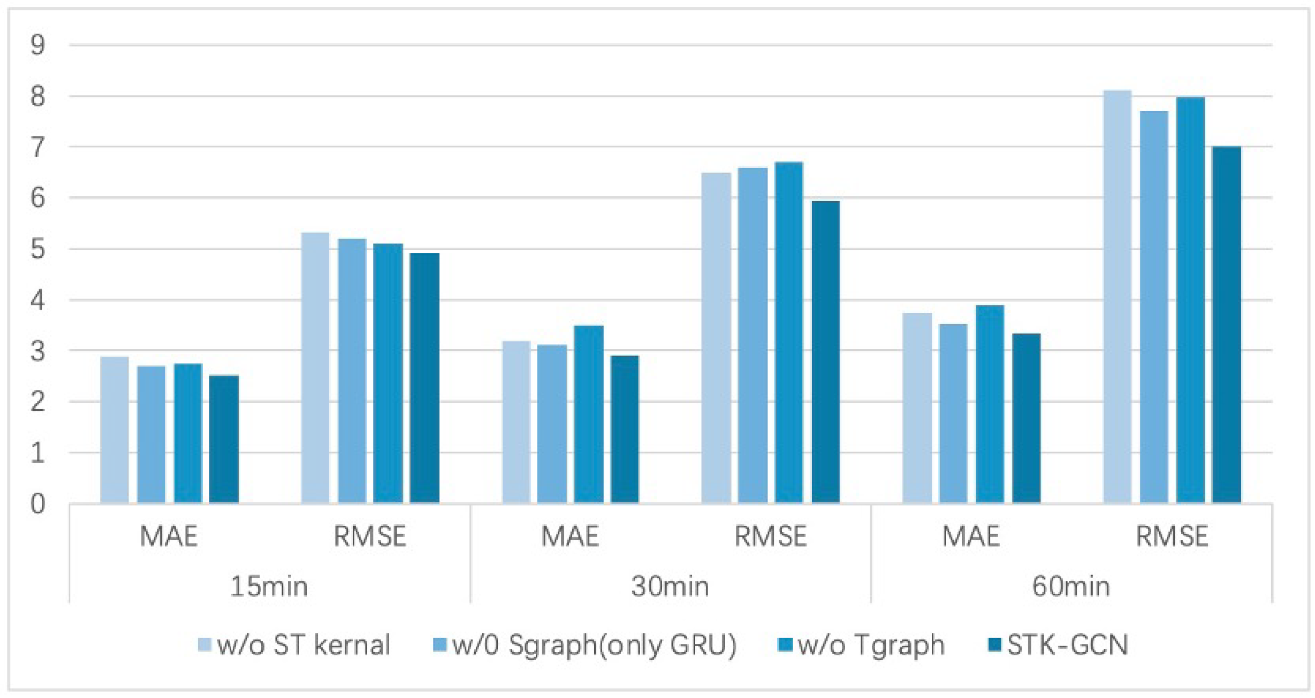
We present a summary of the evaluation results for all methods on traffic flow and speed forecasting tasks in

Table 2. Traffic-forecasting performance.

Dataset	Model	15 min			30 min			60 min
		MAE	RMSE	MAPE	MAE	RMSE	MAPE	MAE	RMSE	MAPE
METR-LA	STGCN	2.88	5.74	7.62%	3.47	7.24	9.57%	4.59	9.40	12.70%
	DCRNN	2.77	5.38	7.30%	3.15	6.45	8.80%	3.60	7.60	10.50%
	GWNet	2.69	5.15	6.90%	3.07	6.22	8.37%	3.53	7.37	10.01%
	MTGNN	2.69	5.18	6.86%	3.05	6.17	8.19%	3.49	7.23	9.87%
	PM-MemNet	2.65	5.29	7.01%	3.03	6.29	8.42%	3.46	7.29	9.97%
	StemGNN	2.56	5.06	6.46%	3.01	6.03	8.23%	3.43	7.23	9.85%
	HOMGNN	2.65	5.06	6.83%	3.02	6.10	8.22%	3.48	7.18	9.94%
	MRA-BGCN	2.67	5.12	6.80%	3.06	6.17	8.30%	3.49	7.30	10.00%
	GMAN	2.77	5.48	7.25%	3.07	6.34	8.35%	3.40	7.21	9.72%
	Traffic transformer	2.66	5.11	6.75%	3.00	6.06	8.00%	3.39	7.04	9.37%
	STK-GCN	2.52	4.91	6.33%	2.91	5.95	7.71%	3.33	7.01	9.28%
PEMSBAY	STGCN	1.36	2.96	2.90%	1.81	4.27	4.17%	2.49	5.69	5.79%
	DCRNN	1.38	2.95	2.90%	1.74	3.97	3.90%	2.07	4.74	4.90%
	GWNet	1.34	2.83	2.79%	1.69	3.80	3.79%	2.00	4.54	4.73%
	MTGNN	1.33	2.80	2.81%	1.65	3.75	3.73%	1.93	4.45	4.58%
	GTS	1.34	2.84	2.83%	1.67	3.83	3.79%	1.98	4.56	4.59%
	PM-MemNet	1.34	2.82	2.81%	1.65	3.76	3.71%	1.95	4.49	4.54%
	HOMGNN	1.32	2.75	2.79%	1.63	3.68	3.71%	1.93	4.42	4.62%
	MRA-BGCN	1.29	2.72	2.90%	1.61	3.67	3.80%	1.91	4.46	4.60%
	GMAN	1.36	2.93	2.88%	1.64	3.78	3.71%	1.90	4.40	4.45%
	Traffic Transformer	1.35	2.82	2.84%	1.66	3.72	3.75%	1.95	4.49	4.65%
	STK-GCN	1.29	2.72	2.70%	1.60	3.67	3.62%	1.89	4.42	4.48%

. For the baselines mentioned above, we use the data reported in each method paper. From Table 2, the following observations can be made:

The METR-LA and PEMS-BAY datasets are widely recognized for their large-scale and real-world characteristics, making them ideal benchmarks for traffic-forecasting models. The test results on the METR-LA and PEMS-BAY datasets effectively demonstrate the model’s applicability in real-world scenarios due to their large-scale, real-world nature, and comprehensive coverage of complex traffic patterns [7,8].

The models can be broadly categorized into three types: models that input predefined graphs, models that utilize adaptive graphs, and models based on transformers. Among the SOTAs, models with adaptive graph, such as GWNet and MTGNN, achieve better performance than graph-dependent models such as DCRNN and STGCN. Our model demonstrated superior performance compared to state-of-the-art methods in nearly all scenarios. It significantly outperforms GNN-based methods (DCRNN and STGCN), which utilize GNN on a fixed graph constructed based on road network distance. Additionally, STK-GCN distinctly outperforms adaptive graph approaches (GWnet and MTGNN), demonstrating the unique contribution of the spatio-temporal kernel.

Compared to the second-best model, StemGNN, STK-GCN exhibits more pronounced advantages in long-term forecasting (60 min), likely attributable to the kernel’s capacity to capture latent dependencies. GWNet incorporates a self-adaptive graph to model hidden spatial dependencies. Our STK-GCN develops this idea and further introduces a novel kernel to generate both spatial and temporal graph matrices, which enhances the feature capture capability of model.

We also compared the $R^2$ values of several important models with those of our model in

Table 3. Comparison of the $R^2$ results of the models.

Model	STGCN	DCRNN	GWNet	GMAN	STK-GCN
$R^2$	0.7351	0.7897	0.8044	0.7968	0.8235

. The data in this table present the overall $R^2$ values for the METR-LA dataset across different models. Specifically, the $R^2$ value of STK-GCN reached 0.8235, which is significantly higher than those of other mainstream models. These results indicate that our model has a stronger ability to explain the variance in the data, capturing key information more accurately than other models.

5. Ablation Study

Ablation test. To verify the effectiveness of the proposed modules, we test three variants of the model on METR-LA. The first one uses two adaptive graph modules to generate spatial and temporal graphs separately instead of the spatio-temporal kernel. The second model eliminates the spatial graph convolution. The third one removes the temporal graph convolution. Table 4 shows the mean MAE, RMSE, and MAPE of three horizons. Figure 5 illustrates the prediction scenarios for three specific time periods.

• without spatio-temporal kernel. This model eliminates the spatio-temporal kernel and instead uses two adaptive graphs.
• without Sgraph. The spatial graph convolution was removed, that is, the graph convolution part in GCRU was eliminated and GRU was used alone.
• without Tgraph. This variant eliminates the temporal graph convolution module, encompassing both the temporal graph convolution and the exponential smoothing components.

Table 4. The experimental results of the original model and its three variants.

Model	MAE	RMSE	MAPE
without ST kernal	3.50	7.16	9.92%
without Sgraph	2.90	6.05	7.93%
without Tgraph	2.89	5.96	7.86%
STK-GCN	2.86	5.90	7.76%

Table 4. The experimental results of the original model and its three variants.

Model	MAE	RMSE	MAPE
without ST kernal	3.50	7.16	9.92%
without Sgraph	2.90	6.05	7.93%
without Tgraph	2.89	5.96	7.86%
STK-GCN	2.86	5.90	7.76%

Figure 5. The results of STK-GCN and its three variants at three time horizons.

Figure 5. The results of STK-GCN and its three variants at three time horizons.

The experimental results reveal that the removal of any module from the STK-GCN results in an increase in the evaluation metrics, underscoring the essential contribution of each module to the model’s overall performance. Among these components, the spatio-temporal kernel is pivotal in augmenting the model’s performance. By simultaneously accounting for both temporal and spatial dimensions, the spatio-temporal kernel effectively captures the intricate spatio-temporal correlations inherent in traffic-flow data, thereby substantially enhancing the model’s ability to predict traffic-flow variations.

In addition to the spatio-temporal kernel, temporal graph convolution and spatial convolution are also integral components of the model. Temporal graph convolution efficiently captures temporal characteristics of traffic flow, including periodic fluctuations in traffic volume and the persistence of traffic congestion, by performing convolution operations along the temporal axis. Spatial convolution, on the other hand, captures spatial associations between different road segments, such as the mutual influence of traffic flow between adjacent segments, by performing convolution operations along the spatial dimension.

As time progresses, the advantages of STK-GCN become increasingly evident, highlighting the significant role of temporal graph convolution in extracting temporal features. Across varying time intervals, temporal graph convolution precisely identifies the temporal evolution patterns of traffic flow, allowing the model to consistently achieve accurate learning and representation of spatio-temporal information within traffic data.

These results collectively validate the integrity and consistency of the STK-GCN architecture. Only when these modules work in concert can STK-GCN fully leverage its strengths in traffic-flow prediction, providing reliable forecasts for traffic conditions.

Parameter analysis. In this section, we perform experiments to investigate the sensitivity of four hyper-parameters within the STK-GCN framework: the dimension of the spatio-temporal kernel, ranging from 6 × 6 to 64 × 64. The order of Chebyshev polynomial in Equation (21), ranging from 2 to 7. The coefficients of the exponential smoothing module in Equation (16), ranging from 0.5 to 1. The number of layers in each GCRU unit, ranging from 1 to 6. Apart from these parameters, all other hyperparameters were kept constant. Figure 6 presents the model’s test results with varying sizes of spatio-temporal kernels on the METR-LA dataset. In these experiments, the model’s performance is measured by two indicators, MAE and MAPE. To thoroughly assess the model’s predictive performance across different time intervals, the computation of MAE and MAPE metrics encompasses the average of prediction outcomes at three distinct time points: 15 min, 30 min, and 60 min.

The experimental findings suggest that the size of the spatio-temporal kernel requires careful tuning within a specific range, as dimensions that are either too large or too small can detrimentally impact the model’s predictive performance. Specifically, the model’s predictive capability attains its optimal state when the spatio-temporal kernel size is configured to 12 × 12. The optimal value for the exponential smoothing coefficient is 0.7.

The order $k=2$ for Chebyshev polynomials in spatial graph convolution is optimal because it strikes a balance between locality and computational efficiency, capturing 2-hop neighbor information without introducing excessive noise or complexity. It mitigates over-smoothing by maintaining a moderate receptive field, ensuring node features retain discriminative power while avoiding premature global influence. It has also low computational complexity, making it suitable for large-scale graph data.

The optimal performance of GCRU with a single layer can be attributed to its ability to balance model complexity and computational efficiency while effectively capturing temporal dependencies in traffic data. A single-layer GCGRU reduces the risk of overfitting, which is particularly important for traffic-forecasting tasks where data patterns can be highly dynamic and noisy.

Efficiency study. The scatter Figure 7 illustrates the relationship between model complexity (number of parameters) and prediction accuracy (overall MAE) for various models. Each point represents a model, with distinct markers differentiating them, and labels indicating their names. We selected the most representative models to compare with our proposed model. The proposed STK-GCN model demonstrates superior performance with an efficient parameter configuration, achieving the lowest overall MAE among all compared methods. Notably, STK-GCN ranks second in terms of parameter efficiency, utilizing only 222,191 parameters. This compact yet highly effective design underscores its ability to accurately capture spatio-temporal dependencies while minimizing computational complexity. The results highlight the model’s optimal balance between efficiency and predictive accuracy, making it a robust and scalable solution for large-scale traffic-forecasting applications.

6. Conclusions

In this study, we introduce a novel traffic-prediction method, STK-GCN. Building upon prior research, we employ a spatio-temporal kernel to model the latent spatio-temporal correlations among nodes and time series, enabling STK-GCN to effectively capture temporal dynamics across varying localities. The temporal graph convolution is also an innovative concept introduced in this paper. In contrast to conventional approaches for temporal feature extraction, the temporal graph convolution models the relationships between different time steps as a temporal graph, thereby uncovering the underlying temporal correlations within traffic data. On two traffic datasets, our model attains state-of-the-art performance. Future work will involve extending our framework to tasks beyond multivariate time-series forecasting, like railway networks, biological domain and so on.

References

1. Li, Z.; Sergin, N.D.; Yan, H.; Zhang, C.; Tsung, F. Tensor Completion for Weakly-Dependent Data on Graph for Metro Passenger Flow Prediction; Association for the Advancement of Artificial Intelligence: Washington, DC, USA, 2020; Volume 34, pp. 4804–4810. [Google Scholar]
2. Hu, J.; Yang, B.; Guo, C.; Jensen, C.S. Risk-aware path selection with time-varying, uncertain travel costs: A time series approach. Int. Conf. Very Large Data Bases 2018, 27, 179–200. [Google Scholar]
3. Figueiredo, L.; Jesus, I.; Machado, J.T.; Ferreira, J.R.; De Carvalho, J.M. Towards the development of intelligent transportation systems. In Proceedings of the ITSC 2001. 2001 IEEE Intelligent Transportation Systems. Proceedings (Cat. No.01TH8585), Oakland, CA, USA, 25–29 August 2001; pp. 1206–1211. [Google Scholar]
4. Jiang, W.; Luo, J. Graph neural network for traffic forecasting: A survey. Expert. Syst. Appl. 2022, 207, 117921. [Google Scholar]
5. Williams, B.M.; Hoel, L.A. Modeling and forecasting vehicular traffic flow as a seasonal ARIMA process: Theoretical basis and empirical results. J. Transp. Eng. 2003, 129, 664–672. [Google Scholar] [CrossRef]
6. Wu, C.H.; Ho, J.M.; Lee, D.T. Travel-time prediction with support vector regression. IEEE Trans. Intell. Transp. Syst. 2004, 5, 276–281. [Google Scholar]
7. Li, Y.; Yu, R.; Shahabi, C.; Liu, Y. Diffusion convolutional recurrent neural network: Data-driven traffic forecasting. arXiv 2017, arXiv:1707.01926. [Google Scholar]
8. Yu, B.; Yin, H.; Zhu, Z. Spatio-temporal graph convolutional networks: A deep learning framework for traffic forecasting. arXiv 2017, arXiv:1709.04875. [Google Scholar]
9. Seo, Y.; Defferrard, M.; Vandergheynst, P.; Bresson, X. Structured sequence modeling with graph convolutional recurrent networks. In Proceedings of the Neural Information Processing: 25th International Conference, ICONIP 2018, Siem Reap, Cambodia, 13–16 December 2018; Proceedings Part I 25. Springer: Cham, Switzerland, 2018; pp. 362–373. [Google Scholar]
10. Cao, D.; Wang, Y.; Duan, J.; Zhang, C.; Zhu, X.; Huang, C.; Tong, Y.; Xu, B.; Bai, J.; Tong, J.; et al. Spectral temporal graph neural network for multivariate time-series forecasting. Adv. Neural. Inf Process. Syst. 2020, 33, 17766–17778. [Google Scholar]
11. Chen, C.; Li, K.; Teo, S.G.; Zou, X.; Wang, K.; Wang, J.; Zeng, Z. Gated residual recurrent graph neural networks for traffic prediction. In Proceedings of the AAAI Conference on Artificial Intelligence, Honolulu, HI, USA, 27 January–1 February 2019; Volume 33, pp. 485–492. [Google Scholar]
12. Diao, Z.; Wang, X.; Zhang, D.; Liu, Y.; Xie, K.; He, S. Dynamic spatial-temporal graph convolutional neural networks for traffic forecasting. In Proceedings of the AAAI Conference on Artificial Intelligence, Honolulu, HI, USA, 27 January–1 February 2019; Volume 33, pp. 890–897. [Google Scholar]
13. Wu, Z.; Pan, S.; Long, G.; Jiang, J.; Zhang, C. Graph wavenet for deep spatial-temporal graph modeling. arXiv 2019, arXiv:1906.00121. [Google Scholar]
14. Shang, C.; Chen, J.; Bi, J. Discrete graph structure learning for forecasting multiple time series. arXiv 2021, arXiv:2101.06861. [Google Scholar]
15. Wu, Z.; Pan, S.; Long, G.; Jiang, J.; Chang, X.; Zhang, C. Connecting the dots: Multivariate time series forecasting with graph neural networks. In Proceedings of the 26th ACM SIGKDD International Conference on Knowledge Discovery & Data Mining, Virtual, 6–10 July 2020; pp. 753–763. [Google Scholar]
16. Stock, J.H.; Watson, M.W. Vector autoregressions. J. Econ. Perspect. 2001, 15, 101–115. [Google Scholar]
17. Van Lint, J.; Van Hinsbergen, C. Short-term traffic and travel time prediction models. Artif. Intell. Appl. Crit. Transp. Issues. 2012, 22, 22–41. [Google Scholar]
18. Rumelhart, D.E.; Hinton, G.E.; Williams, R.J. Learning representations by back-propagating errors. Nature 1986, 323, 533–536. [Google Scholar]
19. Hochreiter, S.; Schmidhuber, J. Long short-term memory. Neural Comput. 1997, 9, 1735–1780. [Google Scholar] [PubMed]
20. Cho, K.; Van Merriënboer, B.; Gulcehre, C.; Bahdanau, D.; Bougares, F.; Schwenk, H.; Bengio, Y. Learning phrase representations using RNN encoder-decoder for statistical machine translation. arXiv 2014, arXiv:1406.1078. [Google Scholar]
21. Vaswani, A.; Shazeer, N.; Parmar, N.; Uszkoreit, J.; Jones, L.; Gomez, A.N.; Kaiser, Ł.; Polosukhin, I. Attention is all you need. Adv. Neural. Inf. Process. Syst. 2017, 30, 6000–6010. [Google Scholar]
22. Fang, Y.; Zhao, F.; Qin, Y.; Luo, H.; Wang, C. Learning all dynamics: Traffic forecasting via locality-aware spatio-temporal joint transformer. IEEE Trans. Intell. Transp. Syst. 2022, 23, 23433–23446. [Google Scholar]
23. Li, S.; Jin, X.; Xuan, Y.; Zhou, X.; Chen, W.; Wang, Y.X.; Yan, X. Enhancing the locality and breaking the memory bottleneck of transformer on time series forecasting. Adv. Neural. Inf. Process. Syst. 2019, 32, 5243–5253. [Google Scholar]
24. Guo, S.; Lin, Y.; Feng, N.; Song, C.; Wan, H. Attention based spatial-temporal graph convolutional networks for traffic flow forecasting. In Proceedings of the AAAI Conference on Artificial Intelligence, Honolulu, HI, USA, 27 January–1 February 2019; Volume 33, pp. 922–929. [Google Scholar]
25. Zhou, H.; Zhang, S.; Peng, J.; Zhang, S.; Li, J.; Xiong, H.; Zhang, W. Informer: Beyond efficient transformer for long sequence time-series forecasting. In Proceedings of the AAAI Conference on Artificial Intelligence, Online, 2–9 February 2021; Volume 35, pp. 11106–11115. [Google Scholar]
26. Zhang, Z.; Cui, P.; Zhu, W. Deep learning on graphs: A survey. IEEE Trans. Knowl. Data Eng. 2020, 34, 249–270. [Google Scholar]
27. Zhou, J.; Cui, G.; Hu, S.; Zhang, Z.; Yang, C.; Liu, Z.; Wang, L.; Li, C.; Sun, M. Graph neural networks: A review of methods and applications. AI Open 2020, 1, 57–81. [Google Scholar]
28. Jiang, R.; Wang, Z.; Yong, J.; Jeph, P.; Chen, Q.; Kobayashi, Y.; Song, X.; Fukushima, S.; Suzumura, T. Spatio-temporal meta-graph learning for traffic forecasting. In Proceedings of the AAAI Conference on Artificial Intelligence, Washington, DC, USA, 7–14 February 2023; Volume 37, pp. 8078–8086. [Google Scholar]
29. Yuan, K.; Liu, J.; Lou, J. Higher-order masked graph neural networks for traffic flow prediction. In Proceedings of the 2022 IEEE International Conference on Data Mining (ICDM), Orlando, FL, USA, 28 November–1 December 2022; pp. 1305–1310. [Google Scholar]
30. Abduljabbar, R.; Dia, H.; Liyanage, S. Machine learning models for traffic prediction on arterial roads using traffic features and weather information. Appl. Sci. 2024, 14, 11047. [Google Scholar] [CrossRef]
31. Alonso-Solorzano, Á.; Pérez-Acebo, H.; Findley, D.J.; Gonzalo-Orden, H. Transition probability matrices for pavement deterioration modelling with variable duty cycle times. Int. J. Pave. Eng. 2024, 24, 2278694. [Google Scholar]
32. Wu, Y.; Pang, Y.; Zhu, X. Evolution of prediction models for road surface irregularity: Trends, methods and future. Constr. Build. Mater. 2024, 449, 138316. [Google Scholar]
33. Hyndman, R.; Koehler, A.B.; Ord, J.K.; Snyder, R.D. Forecasting with Exponential Smoothing: The State Space Approach; Springer Science & Business Media: Berlin/Heidelberg, Germany, 2008. [Google Scholar]
34. Defferrard, M.; Bresson, X.; Vandergheynst, P. Convolutional neural networks on graphs with fast localized spectral filtering. Adv. Neural. Inf. Process. Syst. 2016, 29, 3844–3852. [Google Scholar]
35. Lee, H.; Jin, S.; Chu, H.; Lim, H.; Ko, S. Learning to remember patterns: Pattern matching memory networks for traffic forecasting. arXiv 2021, arXiv:2110.10380. [Google Scholar]
36. Chen, W.; Chen, L.; Xie, Y.; Cao, W.; Gao, Y.; Feng, X. Multi-range attentive bicomponent graph convolutional network for traffic forecasting. In Proceedings of the AAAI Conference on Artificial Intelligence, New York, NY, USA, 7–12 February 2020; Volume 34, pp. 3529–3536. [Google Scholar]
37. Zheng, C.; Fan, X.; Wang, C. GMAN: A Graph Multi-Attention Network for Traffic Prediction. In Proceedings of the AAAI Conference on Artificial Intelligence, New York, NY, USA, 7–12 February 2020; Volume 34, pp. 1234–1241. [Google Scholar]
38. Yan, H.; Ma, X. Learning dynamic and hierarchical traffic spatiotemporal features with transformer. IEEE trans. Intell. Transp. Syst. 2020, 23, 22386–22399. [Google Scholar]
Figure 1. Framework of spatio-temporal kernel graph convolutional network (STK-GCN).
Electronics 14 01410 g001
Figure 2. The development of the adaptive graph.
Electronics 14 01410 g002
Figure 3. The architecture of the temporal graph convolution module.
Electronics 14 01410 g003
Figure 4. The distribution map of sensor locations in the dataset. (a) METR-LA (Los Angeles). (b) PEMS-BAY (San Francisco Bay Area).
Electronics 14 01410 g004
Figure 6. (a) The dimension of the spatio-temporal kernel. (b) The order of Chebyshev polynomial. (c) The coefficients of the exponential smoothing. (d) The number of layers in each GCRU unit.
Electronics 14 01410 g006
Figure 7. Efficiency evaluation.
Electronics 14 01410 g007