SlantNet: A Lightweight Neural Network for Thermal Fault Classification in Solar PV Systems

Abstract

The rapid growth of solar photovoltaic (PV) installations worldwide has increased the need for the effective monitoring and maintenance of these vital renewable energy assets. PV systems are crucial in reducing greenhouse gas emissions and diversifying electricity generation. However, they often experience faults and damage during manufacturing or operation, significantly impacting their performance, while thermal infrared imaging provides a promising non-invasive method for detecting common defects such as hotspots, cracks, and bypass diode failures, current deep learning approaches for fault classification generally rely on computationally intensive architectures or closed-source solutions, constraining their practical use in real-time situations involving low-resolution thermal data. To tackle these challenges, we introduce SlantNet, a lightweight neural network crafted to classify thermal PV defects efficiently and accurately. At its core, SlantNet incorporates an innovative Slant Convolution (SC) layer that utilizes slant transformation to enhance directional feature extraction and capture subtle thermal gradient variations essential for fault detection. We complement this architectural advancement with a thermal-specific image enhancement augmentation strategy that employs adaptive contrast adjustments to bolster model robustness under the noisy and class-imbalanced conditions typically encountered in field applications. Extensive experimental validation on a comprehensive solar panel defect detection benchmark dataset showcases SlantNet’s exceptional performance. Our method achieves a 95.1% classification accuracy while reducing computational overhead by approximately 60% compared to leading models.

1. Introduction

As the global demand for renewable energy continues to surge, solar photovoltaic (PV) installations, ranging from large-scale ground-mounted farms to rooftop systems, are expanding at an unprecedented pace. International Renewable Energy Agency (IRENA) projects that global installed capacity of PV systems will reach approximately 2156 GW by 2030, reflecting significant growth and highlighting the importance of ensuring system reliability [1]. One major challenge in maintaining these installations is fault identification, particularly in vast power plants where manually monitoring individual panels is impractical. Solar PV modules, composed of silicon-based semiconductors, convert photons into electrical power when sunlight interacts with the PV cells. The accumulated cells form a solar array that generates electricity. Over time, various faults and degradations, such as micro-cracks, hotspots, soiling, and bypass diode failures, can critically undermine both energy yield and the long-term reliability of PV systems, with losses due to faults recorded at approximately 17.4% by the National Renewable Energy Laboratory (NREL) in 2022 [1,2,3,4,5].

Furthermore, studies have pointed to the substantial impacts of faults on PV performance; for instance, allowing PV surfaces to remain unclean in dusty environments can decrease power generation by 18% in just one month of dust accumulation [6]. Additionally, long-term degradation studies show power losses of up to 11% over 20 years due to factors such as soldering defects, micro-cracks, shading, and hotspots [6]. Faults in critical components such as the encapsulant and junction box have been identified as particularly severe, contributing significantly to reliability risks in PV installations [7].

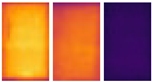
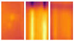
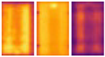
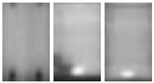
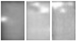
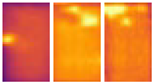
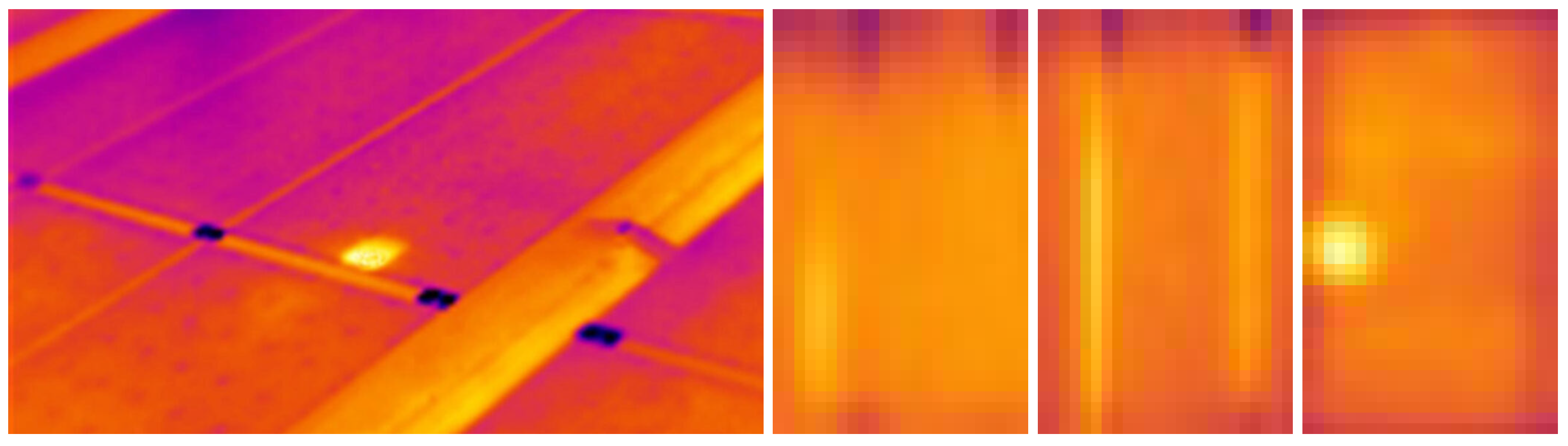
Thermal infrared (IR) imaging has emerged as a vital noninvasive diagnostic approach for identifying faults such as hotspots, cracks, and bypass diode malfunctions, manifesting as localized temperature anomalies on the module surface. Figure 1 illustrates examples of infrared images showing different hotspot defects. Traditionally, fault detection has relied on time-intensive methods like manual inspection or electrical testing [8,9]. However, these approaches are unscalable for large solar farms, prompting the growing adoption of thermal IR imaging techniques for rapid, remote monitoring [10,11,12,13]. Recent advancements in deep learning have substantially enhanced the efficiency and accuracy of classifying PV faults from thermal images, though many existing solutions utilize resource-intensive architectures or proprietary codebases, limiting their applicability for real-time or resource-constrained scenarios [14].

Artificial Intelligence (AI) methods, particularly neural networks, have shown significant potential for reliable fault diagnosis in complex energy systems. For instance, recent studies using AI models for predicting nitrogen oxide emissions in thermal power plants have demonstrated the importance of appropriate feature selection for high predictive accuracy, emphasizing that there are similar benefits for PV fault detection tasks [15]. Despite substantial progress, there remains a clear need for lightweight and computationally efficient deep learning solutions capable of deployment on low-resolution or mobile imaging platforms. This paper introduces SlantNet, a lightweight neural network designed to address this gap. SlantNet leverages the Slant Convolution layer to capture critical directional features and thermal gradients for accurate anomaly detection while employing thermal-specific data augmentation strategies to mitigate class imbalance and enhance robustness. Our work contributes to scalable real-time fault detection, promoting integration into broader renewable energy monitoring systems.

Fast image transforms play an essential role in digital image processing as theoretical and practical tools for numerous tasks, including image filtering, restoration, encoding, and analysis [16]. In particular, the multidimensional discrete Fourier transform (DFT) is widely used for frequency analysis; however, it may not be optimal for purely real data due to its reliance on complex operations. Consequently, transforms like the discrete cosine transform (DCT) and the Slant Transform are often preferred to handle real-value input images [17,18]. The Slant Transform employs a discrete sawtooth-like basis vector, making it incredibly efficient at representing linear brightness variations along an image line [19,20].

The Slant Transform (SLT) is a fast, orthogonal transform that is well suited for analyzing piecewise linear data [19,20,21]. Initially developed for image coding by Enomoto and Shibata, its key characteristics include an orthonormal set of basis vectors (one constant and one “slant” basis vector optimized for linear luminance gradients), a sequence property for frequency analysis, variable size transformation, a fast computational algorithm, and high energy compaction. The SLT finds applications in various image processing tasks, including image compression, denoising, enhancement, and restoration. Our proposed approach uses these strengths by replacing traditional convolutional neural network filters with SLT filters. This novel integration merges the SLT’s computational efficiency and directional sensitivity with the learning capabilities of neural networks, resulting in a more efficient architecture that is particularly valuable for resource-constrained applications like thermal image analysis.

Concurrently, the push for sustainable energy accentuates solar power as a key renewable resource, with PV systems playing a pivotal role in converting sunlight into electricity. Unfortunately, the operational performance of these systems diminishes over time due to the faults above, each posing significant consequences for energy yield and module lifespan [2,3,4]. Thermal imaging is notably effective at detecting hotspots, localized temperature rises that can lead to severe degradation if left unchecked. Ensuring timely and accurate fault detection improves maintenance workflows, reduces long-term costs, and preserves optimal system performance [8,9].

Recent Deep Learning Efforts. Deep learning has opened new possibilities for PV fault classification, prompting the exploration of architectures tailored to domain-specific constraints. Approaches include convolutional neural networks (CNNs) with data augmentation [22], multi-scale CNNs leveraging transfer learning [23], and lightweight coupled UDenseNet models [24] for unbalanced datasets. Enhanced versions of standard architectures, such as a modified MobileNet-V3 [25] and lightweight inception residual networks like LIR-Net [26], further boost classification accuracy while curtailing computational overhead. Furthermore, a cascading decision system designed specifically for thermal image analysis in large-scale PV installations has improved anomaly detection by effectively addressing data imbalance in UAV-acquired datasets [27]. Collectively, these efforts reinforce the need for the efficient, scalable classification of thermal imagery. However, many of these models suffer from significant shortcomings as follows: they are often too resource-intensive for real-time applications; lack customization for the unique challenges of thermal images, such as blurriness, low resolution, and low contrast; and are frequently accompanied by limited or unavailable open source code bases, thereby hindering reproducibility and industrial adoption.

Proposed Approach. Motivated by the inherent challenges in thermal imaging for solar panel fault detection, namely, blurry, low-resolution and low-contrast images, we introduce SlantNet, a lightweight neural network designed for automatic fault identification and classification using thermal imagery. This innovative approach enhances PV system reliability and performance while reducing operational costs through two key technical advances as follows: (i) a thermal-specific image enhancement and augmentation framework that employs adaptive contrast improvement and decolorization techniques to mitigate noise and compensate for low image quality, and (ii) a novel framework incorporating a 2D Slant Transform layer that leverages a fixed harmonic basis to capture directional features and subtle intensity gradients essential for IR-based diagnostics, thereby surpassing the capabilities of traditional CNN architectures.

The main contributions of this research are as follows:

• We developed an innovative Slant Convolution layer that harnesses the power of the Slant Transform to extract robust directional features from low-resolution thermal images. This specialized layer detects subtle fault signatures that conventional approaches often overlook.
• We created a lightweight, efficient neural network architecture optimized for real-time deployment on resource-constrained devices. SlantNet achieves 95.1% classification accuracy compared to state-of-the-art models while reducing computational requirements by 60%, making it ideal for field deployment.
• We implemented a novel image enhancement and augmentation framework that combines two complementary, measure-driven contrast enhancement techniques. The framework employs adaptive contrast stretching and optimal decolorization to significantly improve image quality and model robustness under challenging conditions, achieving a 2–5% improvement in fault detection accuracy for noisy and class-imbalanced scenarios.
• We validated a comprehensive dataset for detecting solar panel defects through extensive experiments. Our benchmarking against top models shows that SlantNet outperforms others, achieving faster inference times and greater accuracy across various fault categories while lowering computational overhead.

The remainder of this article is organized as follows. Section 2 presents an overview of the related work and the evolution of neural networks for thermal PV fault detection. Section 3 details the proposed SlantNet architecture and the thermal-specific augmentation strategies. Section 4 provides the experimental results, benchmark comparisons, and a discussion of the key findings. Lastly, Section 5 concludes the paper and outlines future research directions.

2. Background

Deep learning has revolutionized image classification across various domains, including PV fault detection. However, standard models are often resource-intensive. We briefly describe the architectures considered in our comparative analysis, as follows:

• AlexNet [28]: A pioneering CNN architecture that introduced deep learning to large-scale image classification. Although effective, it is parameter-heavy.
• ResNet50 [29]: Employs residual connections to overcome vanishing gradients, enabling very deep networks. Highly accurate but computationally costly.
• SqueezeNet [30]: Focuses on parameter reduction using “squeeze” and “expand” layers, achieving AlexNet-level accuracy with significantly fewer parameters.
• ShuffleNetV2 [31]: Improves efficiency through channel splitting and channel shuffle operations, well suited for mobile and low-power devices.
• MobileNetV3 [32]: Optimized for mobile applications, using depthwise separable convolutions and squeeze–excite modules to reduce computational load.
• EfficientNet [33]: EfficientNet introduces a compound scaling method that uniformly scales network depth, width, and resolution, leading to state-of-the-art performance while significantly reducing computational cost. This balanced design allows it to achieve high accuracy on image classification tasks with fewer parameters and FLOPs compared to traditional architectures.
• Vision Transformer (ViT) [34]: Leverages transformer blocks for image classification, but typically requires large training datasets and more computing.
• Swin Transformer [35]: A hierarchical transformer architecture that computes representations at various scales, yielding state-of-the-art results with higher computational overhead.

While these models have advanced the field, most of them often remain challenging to deploy for real-time PV fault detection on low-resolution, noisy thermal images.

Several studies have addressed the challenges of solar panel fault classification using deep learning and thermal imaging techniques. CNNs have been a central approach, as demonstrated by Alves et al. [22], who utilized infrared thermography combined with data augmentation to classify multiple defect classes in PV modules. Their method effectively handled unbalanced datasets and highlighted the within-class and between-class variation challenges. Similarly, Korkmaz et al. [23] proposed a multi-scale CNN with transfer learning, using multiple convolutional branches to improve feature representation. Their approach employed offline augmentation techniques to address dataset imbalance and demonstrated robust performance across various fault types, such as cracks and diode failures.

Building on lightweight architectures, Pamungkas et al. [24] introduced a coupled UDenseNet model, leveraging geometric transformations and image augmentation using a Generative Adversarial Network (GAN) to achieve high accuracy, making it suitable for large-scale solar farms. Another study explores the efficiency of a lightweight convolutional neural network for classifying thermal images, achieving high accuracy by transforming low-dimensional images using various feature extraction methods [36]. Tang et al. [25] proposed modifications to the MobileNet architecture, enhancing preprocessing and data augmentation to improve performance on noisy and limited datasets, achieving faster inference and higher recognition rates for diverse fault types. Lee et al. [26] developed LIRNet. This lightweight inception residual network incorporated hierarchical learning and K-means clustering to refine datasets and improve fault detection accuracy and speed compared to EfficientNet.

These advancements collectively emphasize the importance of tailored deep learning architectures, data augmentation, and preprocessing techniques in improving the robustness and efficiency of PV fault classification. Our proposed method builds on these innovations by integrating the Slant Transform, enhancing feature extraction and ensuring efficient operation on low-resolution thermal images.

3. Proposed Method

In this section, we present our proposed method, which combines Slant Convolution for enhanced feature extraction, a lightweight model architecture tailored for real-time thermal image processing, and thermal-specific data augmentation techniques to address the challenges of PV fault detection in low-resolution thermal images.

3.1. Slant Convolution

Harmonic convolution layers, as introduced in previous studies, replace traditional convolutional layers by leveraging predefined spectral filters to capture frequency domain features instead of learning spatial filters from scratch [37,38,39]. These layers decompose input features into spectral components using transformations such as the Discrete Cosine Transform (DCT), allowing networks to learn optimal combinations of preset feature extractors. This approach reduces the risk of overfitting, decreases computational complexity, and enhances the extraction of rich frequency domain features. Inspired by this principle, we incorporate the Slant Transform as a harmonic layer in our network, specifically designed to excel at capturing linear intensity variations and directional patterns in images. By incorporating these enhanced filters into convolutional layers, the network can more effectively emphasize subtle fault signatures that standard kernels may overlook.

The Slant Transform (SLT) is a rapid, orthogonal transform ideal for analyzing piecewise linear data. Initially developed for image coding by Enomoto and Shibata in 1971 and further refined by Pratt et al. and Agaian et al., the SLT provides advantages in computational efficiency and hardware implementation, sharing properties with cosine and Fourier transforms [19,20,40]. Its key characteristics include an orthonormal set of basis vectors (comprising one constant and one “slant” basis vector optimized for linear luminance gradients), a sequence property for frequency analysis, variable size transformations, a fast computational algorithm, and high energy compaction.

A significant strength of the SLT is its ability to match basis vectors to areas of constant luminance slope. This makes it highly effective for capturing directional image features. Although its energy compaction might be sub-optimal compared to some transforms, the SLT’s reduced processing time and more straightforward hardware implementation compared to DCT and DWT make it attractive. This efficiency and directional feature capture make the SLT well suited for real-time image processing.

The SLT has found applications in various image processing tasks, including image compression, denoising, enhancement, and restoration. Our proposed approach utilizes these strengths by substituting traditional convolutional neural network filters with SLT filters. This innovative integration combines the SLT’s computational efficiency and directional sensitivity with the learning capabilities of neural networks, resulting in a more efficient architecture that is particularly advantageous for resource-constrained applications such as thermal image analysis. We connect classical image processing and deep learning by incorporating the SLT into the neural network architecture. This synthesis amalgamates the SLT’s computational efficiency and mathematical properties with the learning power of neural networks. Ultimately, this approach yields a more effective and efficient solution for thermal image analysis, especially for applications like solar panel fault detection.

Mathematically, the Slant Transform is defined by an orthogonal transform matrix applied to image blocks. For $N=2^n$, the transform matrix ${\mathbf{S}}_N$ is constructed as shown in Equation (1). This matrix generates the basis functions using a recursive method, starting from a small matrix in the base case and building up to higher dimensions via the following recursive relationship [20,21]:

$${\mathbf{S}}_N={\displaystyle \frac{1}{\sqrt{2}}}\left[\begin{array}{cccccccc}1& & 0& & 1& & 0& \\ & & & \mathbf{0}& & & & \mathbf{0}\\ a_N& & b_N& & -a_N& & b_N& \\ & \mathbf{0}& & {\mathbf{I}}_{(N/2)-2}& & \mathbf{0}& & {\mathbf{I}}_{(N/2)-2}\\ 0& & 1& & 0& & -1& \\ & & & \mathbf{0}& & & & \mathbf{0}\\ -b_N& & a_N& & b_N& & a_N& \\ & \mathbf{0}& & {\mathbf{I}}_{(N/2)-2}& & \mathbf{0}& & -{\mathbf{I}}_{(N/2)-2}\end{array}\right]\left[\begin{array}{cc}{\mathbf{S}}_{N/2}& \mathbf{0}\\ \mathbf{0}& {\mathbf{S}}_{N/2}\end{array}\right],$$

(1)

$${\mathbf{S}}_2={\displaystyle \frac{1}{\sqrt{2}}}\left[\begin{array}{cc}\hfill 1& \hfill 1\\ \hfill 1& \hfill -1\end{array}\right],$$

(2)

$$a_{2N}={\left({\displaystyle \frac{3N^2}{4N^2-1}}\right)}^{1/2},b_{2N}={\left({\displaystyle \frac{N^2-1}{4N^2-1}}\right)}^{1/2},N=2^n,n\ge 1,$$

(3)

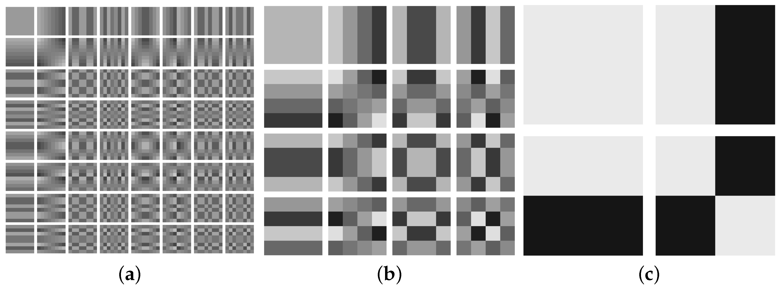
where ${\mathbf{I}}_N$ is the identity matrix of order $N\times N$. The primary advantage of the Slant Transform lies in its effectiveness in representing gradual intensity changes within images, particularly linear increases or decreases in pixel values. Figure 2 provides visual examples of the base filters generated using Slant transformation matrices of sizes $2\times 2$, $4\times 4$, and $8\times 8$. These filters act as fundamental building blocks for analyzing images, enabling the extraction of essential features that capture both uniform intensity regions and subtle intensity transitions. Such transitions are particularly relevant for detecting faults in solar PV modules, where anomalies often manifest as gradual thermal gradients or distinct intensity patterns.

To further enhance feature extraction, we incorporate the Slant Convolution (SC) layer into our network. Unlike standard convolutional layers, which directly learn spatial filters from data, the SC layer first decomposes the input image into a transform domain using a fixed Slant Transform basis. As illustrated in Figure 2, this fixed basis effectively captures directional and frequency characteristics inherent in the image, providing a structured set of preset feature extractors. Because the Slant Transform is linear, the forward pass through the SC layer closely resembles a conventional convolution operation, enabling gradients to propagate similarly during backpropagation. Notably, the SC layer maintains the same number of parameters as a standard convolutional layer, excluding any additional enhancement parameters ($\gamma$ and $\alpha$) used for adaptively weighting the fixed harmonic filters. Specifically, for an $8\times 8$ transform, each of the 64 fixed basis filters is associated with these trainable parameters, allowing the network to learn and emphasize the relative importance of the predefined harmonic features. Thus, the SC layer can be viewed as a specialized form of depth-separable convolution, where spatial filters are predetermined, and their relative contributions are adaptively modulated.

The enhancement is applied via a logarithmic equation, expressed as follows:

$$\tilde{M}=log{\left(1+M^{\gamma }\right)}^{\alpha },$$

(4)

where M denotes the magnitude of a given Slant coefficient [41]. After enhancement, the original sign of each coefficient is restored to form the effective filters. This adaptive enhancement allows the network to selectively emphasize spectral features and directional intensity variations, which are crucial for detecting subtle fault signatures.

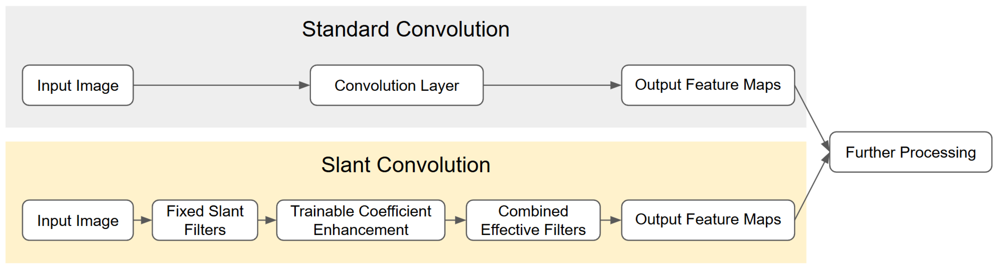
Figure 3 illustrates a comparison between two distinct processing pipelines. In the standard convolution pipeline, learned kernels are directly applied to the input image to extract spatial features. In contrast, the Slant Convolution pipeline first transforms the input image into a spectral representation using a fixed harmonic basis, then adaptively modulates these spectral components through trainable logarithmic enhancement parameters. This structured approach leverages a predefined basis to yield a more interpretable decomposition of image features, significantly improving the network’s ability to capture and respond to subtle directional and frequency-dependent patterns in the data.

3.2. Model Architecture

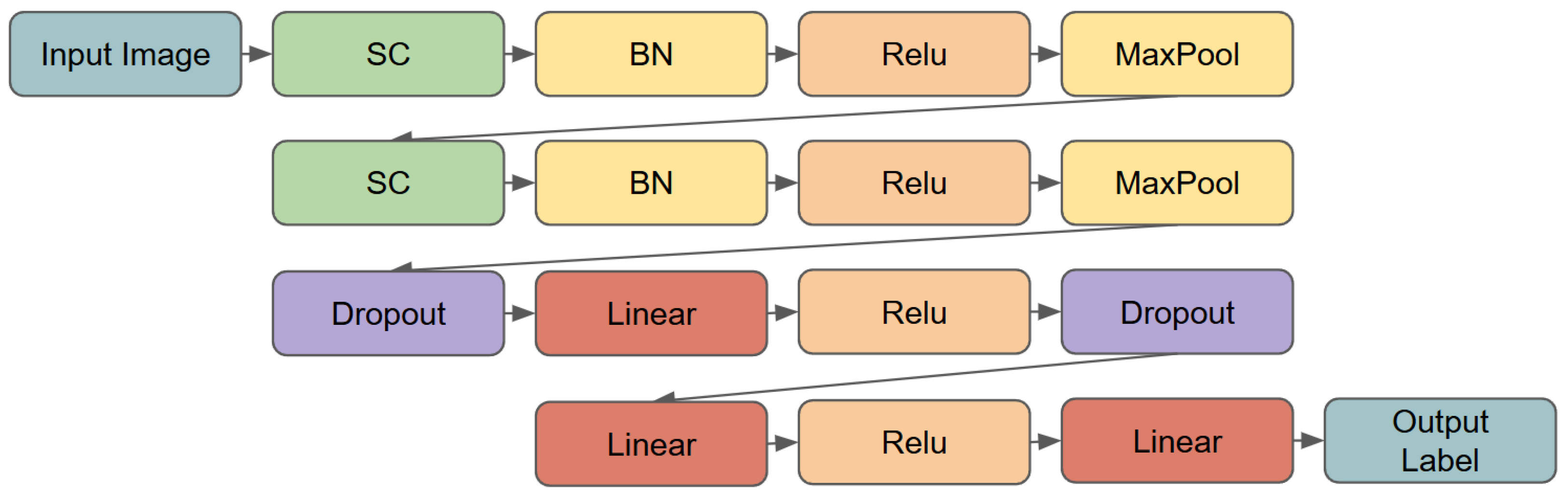
The proposed SlantNet model is designed to effectively classify thermal images into distinct categories. The architecture incorporates a Slant Transform layer when enabled, enhancing feature extraction by capturing directional and geometric patterns within the thermal images. This lightweight architecture is structured to balance computational efficiency and classification accuracy, making it suitable for low-resolution images of size $40\times 40$.

Figure 4 illustrates the overall structure of the network, comprising two convolutional blocks, max-pooling layers, and a fully connected classifier. Below, we describe the architecture in detail, along with the parameters and output dimensions for each layer.

Slant Convolutional (SC) Blocks. The network starts with two convolutional blocks, each consisting of an SC layer followed by batch normalization, a ReLU activation function, and a max-pooling operation, as follows:

• First SC block: The first layer uses 16 filters with a kernel size of $8\times 8$, a stride of 1, and padding of 4 to maintain the spatial dimensions. Batch normalization is applied to stabilize training, followed by ReLU activation. A max-pooling layer reduces the spatial dimensions from $40\times 40$ to $20\times 20$.
• Second SC block: The second layer employs 32 filters with a kernel size of $4\times 4$, a stride of 1, and padding of 2. Like the first block, batch normalization, ReLU activation, and max-pooling are applied, reducing the spatial dimensions from $20\times 20$ to $10\times 10$.

Fully Connected Classifier. After the convolutional blocks, the feature map is flattened to a vector of size $32\times 10\times 10=3200$. This vector is passed through a fully connected classifier consisting of the following layers:

• A dropout layer with a probability of 0.5, followed by a fully connected layer with 1024 neurons and ReLU activation.
• Another dropout layer with a probability of 0.5, followed by a fully connected layer with 64 neurons and ReLU activation.
• A final fully connected layer maps the 64-dimensional vector to the desired number of classes, producing the output logits.

Layer Details.

Table 1. Layer-by-layer details of the SlantNet model.

Layer	Kernel Size	Stride	Output Size
Input	-	-	$1\times 40\times 40$
SC + BN + ReLU	$8\times 8$	1	$16\times 40\times 40$
MaxPool1	$2\times 2$	2	$16\times 20\times 20$
SC + BN + ReLU	$4\times 4$	1	$32\times 20\times 20$
MaxPool2	$2\times 2$	2	$32\times 10\times 10$
Flatten	-	-	3200
FC1 + ReLU + Dropout	-	-	1024
FC2 + ReLU + Dropout	-	-	64
FC3 (Output)	-	-	num_classes

summarizes the parameters and output dimensions of each layer in the SlantNet model. The architecture leverages the Slant Transform in the convolutional layers, enhancing the ability to capture geometric and directional patterns within the input thermal images. With its lightweight design, the model efficiently processes low-resolution images while achieving high classification accuracy, making it suitable for real-time deployment on edge devices.

3.3. Data Augmentation for Thermal Dataset

The dataset used in this study, described in

Table 2. Summary of the Infrared Solar Module Dataset. Each row represents one of the 12 classes (indicated by its class number), the number of images in that class, a brief description, and representative grayscale and colored examples [9].

Class Name [Class Number]	Number of Images	Description	Gray Examples	Colored Examples
No-Anomaly [0]	10,000	Nominal solar modules without faults.
Cell [1]	1877	Hot spot occurring with a square geometry in a single cell.
Cell-Multi [2]	1288	Hot spots occurring with a square geometry in multiple cells.
Cracking [3]	941	Module anomaly caused by cracking on the module surface.
Hot-Spot [4]	251	Hot spot on a thin film module.
Hot-Spot-Multi [5]	247	Multiple hot spots on a thin film module.
Shadowing [6]	1056	Sunlight obstructed by vegetation, structures, or adjacent rows.
Diode [7]	1499	Activated bypass diode, typically affecting 1/3 of the module.
Diode-Multi [8]	175	Multiple activated bypass diodes, typically affecting 2/3 of the module.
Vegetation [9]	1639	Panels blocked by vegetation.
Soiling [10]	205	Dirt, dust, or other debris on the module surface.
Offline-Module [11]	828	Entire module is heated.

, comprises 20,000 thermal images evenly split between anomaly and non-anomaly classes [9]. It includes 11 distinct types of anomalies, such as hotspots, cracks, and bypass diode failures, which are critical for detecting the usage of thermal imaging due to their direct impact on energy efficiency and potential long-term damage. Certain defects, like hotspots, manifest as localized temperature increases and are particularly amenable to detection via infrared imaging. As shown in Table 2, the class distribution is imbalanced; the No-Anomaly class has 10,000 images (half of the dataset), while some anomalies, such as Soiling (205 images) and Diode-Multi (175 images), are heavily underrepresented. This imbalance poses additional challenges for training robust models, as fewer samples are available for certain fault categories.

Data augmentation plays a crucial role in enhancing model performance, especially when working with limited or imbalanced datasets [42], while traditional augmentation techniques (e.g., geometric flips and brightness adjustments) have been widely adopted to improve diversity and robustness [23,24], additional strategies are needed to overcome challenges such as low contrast and the preservation of fine structural details in thermal images.

In our approach, we integrate geometric transformations with thermal quality measure-based enhancements to effectively augment the dataset, inspired by the strategy described in [43]. Specifically, the BIE metric introduced in a study by Ayunts et al. [44] guides the contrast enhancement process, while heatmap decolorization is performed using the TIA no-reference decolorization quality measure [45]. Such measure-based enhancement techniques have been successfully utilized in various image processing tasks to boost image quality and machine learning performance [46]. Our augmentation process comprises the following steps:

• Geometric transformations: The dataset is augmented by applying vertical flips, horizontal flips, and combined flips. These transformations increase the spatial diversity of the training data.
• Contrast enhancement: Each thermal image is subjected to parametric contrast stretching to improve its overall contrast. The low and high stretching parameters are selected from the ranges $[0,150]$ and $[150,255]$, respectively, based on the BIE quality measure. For each image, the two contrast-enhanced versions (corresponding to the highest and second-highest BIE values) are added to the augmented dataset along with the original image.
• Contrast-preserving decolorization: Thermal images are first converted into heatmaps using OpenCV’s INFERNO color map. An optimal decolorization process, guided by the TIA quality measure, is then applied to the heatmaps to enhance contrast while preserving critical structural details.

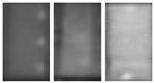
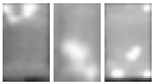
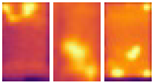
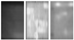
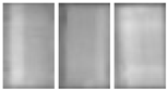
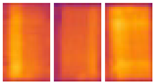
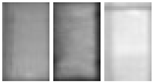
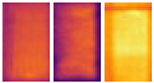
Figure 5 shows an example of an augmented thermal image of a faulty solar panel exhibiting soiling defects, including examples of geometric transformations, contrast-enhanced versions (via quality measure-based enhancement), and the decolorized heatmap.

To ensure effective training, the original dataset consisting of 20,000 images was split into 80% for training (16,000 images) and 10% each for validation and testing (2000 images each). Data augmentation was applied only to the training set as follows: geometric transformations were performed on the entire training set, while contrast enhancement was restricted to faulty images. This strategy not only balanced the dataset but also improved the visual representation of anomalies, increasing the training set size from 16,000 to 88,000 images and significantly boosting the model’s generalization and fault detection capabilities. The sizes of the validation and testing sets remained unchanged to prevent any artificial inflation of accuracy.

4. Results and Discussion

In this section, we present a comprehensive evaluation of the proposed method. The experimental setup and evaluation metrics are first described, followed by a detailed analysis of the quantitative results. We also include ablation studies to assess the contributions of individual components and evaluate the computational efficiency of the proposed architecture compared to existing methods.

4.1. Experimental Setup

All experiments were conducted on a high-performance workstation equipped with an NVIDIA GeForce RTX 4070 Ti SUPER GPU featuring 12 GB of GDDR6X memory (manufactured by ASUSTek Computer Inc., Taipei City, Taiwan), delivering exceptional computational capabilities for deep learning tasks and high-throughput inference. The system was powered by an Intel Core i7-13700K processor (manufactured by Intel Corporation, Santa Clara, California, USA), which includes 16 cores (8 performance cores and 8 efficiency cores) with a maximum clock speed of 5.4 GHz, ensuring efficient data processing and rapid model training. Additionally, the workstation was equipped with 32 GB of DDR5 RAM (Corsair Gaming, Inc., Milpitas, California, USA), enabling it to handle memory-intensive operations such as managing large datasets and training complex neural networks. This setup offered a robust and well-balanced architecture for executing computationally demanding tasks, ensuring consistent and reliable evaluations of the proposed model and its benchmarks.

For training the models, we employed consistent hyperparameters across all experiments. Each model was trained for 50 epochs using the Cross-Entropy loss function, with the training process monitored via validation loss. Training was halted when an increase in validation loss was observed (i.e., early stopping), and the model state corresponding to the best (lowest) validation loss was selected for the final comparisons. The optimization process was carried out using the Adam optimizer, initialized with a learning rate of 0.001. To manage overfitting and enhance convergence, a StepLR learning rate scheduler was utilized, with a step size of 10 epochs and a gamma factor of 0.5 to progressively reduce the learning rate. The batch size for all experiments was set to 32 to ensure a balance between computational efficiency and gradient stability.

Additionally, no pretrained weights were used for any of the models; all were implemented using the torchvision module of PyTorch (version 2.0.1, built with CUDA 12.1) Where necessary, architectures were minimally adapted to accommodate the specific number of output classes for the classification task.

Due to the lack of available codebases and detailed experimental setups for existing thermal-specific models, it is challenging to reproduce their results or make fair comparisons. Given that our proposed model introduces improved convolution layers designed specifically for thermal image analysis, we opted to benchmark against popular, well-established CNN-based and transformer-based architectures. Specifically, we selected the latest and most lightweight versions, such as MobileNetV3 and the tiny variant of Swin Transformer, to ensure efficient, fair, and reproducible comparisons.

4.2. Evaluation Metrics

To assess the performance of the proposed fault classification model for thermal images, we utilized the following four key evaluation metrics: accuracy, precision, recall, and specificity [47]. These metrics provide a comprehensive evaluation framework, particularly useful in cases with class imbalances, as they highlight different aspects of the model’s performance.

Accuracy measures the overall correctness of the model, representing the proportion of total correct predictions. It is calculated as follows:

$$\mathrm{Accuracy}={\displaystyle \frac{TP+TN}{TP+TN+FP+FN}}$$

(5)

where $TP$ (True Positives) and $TN$ (True Negatives) represent correctly identified faulty and non-faulty instances, respectively, while $FP$ (False Positives) and $FN$ (False Negatives) denote incorrect classifications. Although accuracy provides a general indication of performance, it may not fully reflect model effectiveness in cases of class imbalance.

Precision quantifies the proportion of correctly classified positive cases (faults) out of all instances predicted as positive. High precision implies a low false positive rate, ensuring that most identified faults are genuine. Precision is defined as follows:

$$\mathrm{Precision}={\displaystyle \frac{TP}{TP+FP}}$$

(6)

Recall, or sensitivity, measures the model’s ability to identify all relevant instances of faults. A high recall value indicates that the model successfully detects most actual faults, minimizing missed detections. It is defined as follows:

$$\mathrm{Recall}={\displaystyle \frac{TP}{TP+FN}}$$

(7)

Specificity, also known as the True Negative Rate (TNR), evaluates the model’s ability to correctly identify non-faulty instances, thus reducing false positives. Specificity is crucial in contexts where falsely flagged non-faulty cases could lead to unnecessary interventions. It is calculated as follows:

$$\mathrm{Specificity}={\displaystyle \frac{TN}{TN+FP}}$$

(8)

Together, these metrics provide a balanced evaluation of the model’s performance, while accuracy gives an overall measure, precision and recall focus on the model’s capability to correctly identify true faults without generating excessive false positives or missing actual faults. Specificity complements these by verifying the model’s effectiveness in correctly classifying non-faulty instances, providing a well-rounded understanding of the model’s behavior in a real-world PV fault detection scenario.

4.3. Quantitative Results

Table 3. Classification performance on the validation and test sets for binary classification. The best performing metrics are highlighted in bold.

Model	Test				Validation
	Acc	Pr	Rec	Sp	Acc	Pr	Rec	Sp
AlexNet	92.45	93.21	91.63	93.27	92.80	94.31	91.11	94.49
ResNet50	92.65	92.98	92.33	92.97	92.05	92.18	91.91	92.19
SqueezeNet	89.60	92.25	86.55	92.67	88.75	92.08	84.82	92.69
ShuffleNetV2	92.95	93.02	92.93	92.97	92.20	93.07	91.21	93.19
MobileNetV3	93.30	93.07	93.63	92.97	92.95	93.26	92.61	93.29
EfficientNet	93.50	94.87	92.03	94.98	94.05	95.37	92.61	95.50
ViT	88.05	89.80	85.96	90.16	88.40	90.69	85.61	91.19
Swin	91.35	92.27	90.34	92.37	91.75	93.36	89.91	93.59
Proposed	95.10	95.48	94.72	95.48	94.35	95.40	93.21	95.50

summarizes the classification performance of various models on the validation and test sets for binary tasks, while

Table 4. Classification performance on the validation and test sets for 12-class classification. The best performing metrics are highlighted in bold.

Model	Test				Validation
	Acc	Pr	Rec	Sp	Acc	Pr	Rec	Sp
AlexNet	77.50	61.41	58.50	97.61	77.95	65.40	60.16	97.59
ResNet50	78.75	66.45	62.56	97.68	78.35	67.32	60.94	97.62
SqueezeNet	76.70	62.46	57.41	97.46	77.85	67.20	59.16	97.49
ShuffleNetV2	79.30	66.43	62.59	97.78	80.65	72.32	64.00	97.82
MobileNetV3	82.10	68.11	67.92	98.11	81.60	71.32	64.93	98.05
EfficientNet	82.20	69.37	71.05	98.19	82.55	72.35	69.51	98.18
ViT	74.70	60.60	54.76	97.17	75.65	65.26	57.57	97.16
Swin	80.45	65.93	63.19	97.98	81.55	71.61	66.77	98.02
Proposed	82.75	69.52	66.83	98.15	84.30	74.06	66.67	98.28

details the results for the 12-class classification tasks. The performance metrics include accuracy (Acc), precision (Pr), recall (Rec), and specificity (Sp). These metrics provide a comprehensive evaluation of each model’s ability to detect and classify faults in PV modules effectively.

From the results, it is evident that our proposed model outperforms all other models in binary classification, achieving the highest accuracy (95.10%), precision (95.48%), recall (94.72%), and specificity (95.48%) on the test set. This indicates the model’s robustness in distinguishing between anomaly and non-anomaly cases with minimal misclassification. Similarly, in the 12-class classification task, our model demonstrates competitive performance, with an accuracy of 82.75% and the highest precision (69.52%) on the test set. Although MobileNetV3, EfficientNet, and Swin achieve slightly higher recall in some cases, our model maintains a strong balance across all metrics.

In comparison, SqueezeNet and transformer-based models ViT and Swin generally perform less effectively, particularly in the 12-class classification task, where they struggle to maintain high precision and accuracy. This reinforces the suitability of lightweight CNN architectures, such as our proposed model, for thermal image classification tasks. AlexNet, a traditional CNN model, demonstrates moderate performance but surpasses more recent and efficient architectures like ShuffleNetV2 and MobileNetV3.

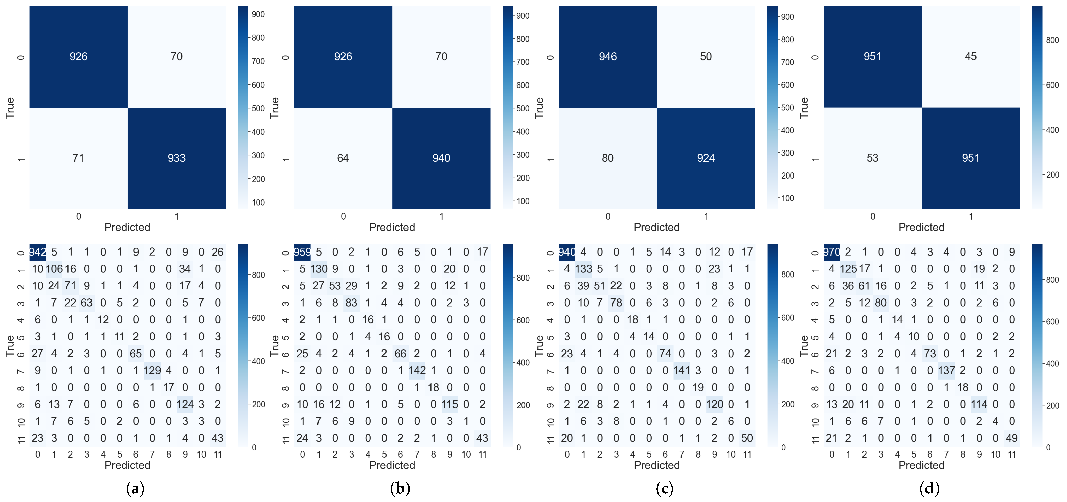
In Figure 6, we illustrate the training loss per iteration for the four top-performing models (ShuffleNetV2, MobileNetV3, EfficientNet, and SlantNet). Meanwhile, Figure 7 presents the confusion matrices for both binary and 12-class classification tasks, providing a detailed visualization of how these same models distribute their predictions across different classes. In the 12-class classification case, we observe that Classes 2 (Cell-Multi) and 11 (Offline-Module) exhibit higher misclassifications, primarily due to their visual similarities with Class 1 (Cell) and Class 0 (No-Anomaly), respectively. Based on these misclassification patterns, we assume that a similar challenge arises in the binary classification scenario, where faulty samples can be misclassified as non-faulty, mainly, instances of the Offline-Module class that are frequently mistaken for No-Anomaly. Additionally, classes 4 (Hot-spot), 5 (Hot-spot-multi), and 10 (Soiling) are underrepresented in the original dataset (see Table 2), resulting in fewer training examples and, consequently, lower recall scores. Addressing these challenges through alternative sampling strategies and improved data augmentation techniques will be the focus of our future work.

4.4. Ablation Studies

In this section, we analyze the contributions of key components in our approach through ablation studies. Specifically, we evaluate the importance of the Slant Convolution layer and the proposed dataset augmentation techniques.

Table 5. Comparison of Conv2d and the proposed Slant Convolution (SC) in terms of test loss and accuracy during the training.

	Convolution	Binary			12 Classes
		Epoch1	Epoch10	Epoch30	Epoch1	Epoch10	Epoch30
Loss	Conv2d	0.3483	0.2026	0.1569	0.9596	0.6361	0.5414
	SC	0.3163	0.1803	0.1468	0.8816	0.5831	0.5224
Accuracy	Conv2d	84.7	92.95	94.8	69.6	79.2	82.25
	SC	87.3	93.05	95.1	70.8	79.75	82.39

compares the performance of standard Conv2d layers with the proposed Slant Convolution layers in terms of test loss and accuracy across epochs for binary and 12-class classification tasks. The results clearly highlight the superiority of the Slant Convolution in capturing directional and intensity-gradient information. For binary classification, the Slant Convolution achieves a higher accuracy across all epochs compared to Conv2d. Similarly, for the 12-class task, the Slant Convolution reduces loss to 0.5224 and improves accuracy to 82.39%, demonstrating its effectiveness in handling more complex fault classifications.

Table 6. Ablation studies for dataset augmentation. Classification results for the validation set with and without proposed dataset augmentation. The best performing metrics are highlighted in bold.

Model	Augmentation	Binary				12 Classes
		Acc	Pr	Rec	Sp	Acc	Pr	Rec	Sp
ResNet50	No Aug	90.60	93.11	87.71	93.49	78.95	69.97	58.98	97.68
	Proposed	92.05	92.18	91.91	92.19	78.35	67.32	60.94	97.62
ShuffleNetV2	No Aug	90.45	92.19	88.41	92.49	77.05	66.05	55.95	97.36
	Proposed	92.20	93.07	91.21	93.19	77.85	67.20	59.16	97.49
MobileNetV3	No Aug	92.35	94.35	90.11	94.59	79.80	69.87	62.19	97.79
	Proposed	92.95	93.26	92.61	93.29	81.60	71.32	64.93	98.05
EfficientNet	No Aug	93.65	94.32	92.91	94.39	82.85	73.22	68.79	98.14
	Proposed	94.05	95.37	92.61	95.50	82.55	72.35	69.51	98.18
SlantNet	No Aug	93.50	94.76	92.11	94.89	80.30	70.14	62.17	97.83
	Proposed	94.35	95.40	93.21	95.50	84.30	74.06	66.67	98.28

evaluates the impact of the proposed dataset augmentation techniques on the classification performance of different models. Without augmentation, the models generally exhibit lower accuracy, precision, and recall across both binary and 12-class classification tasks. For instance, SlantNet achieves 94.35% accuracy in binary classification with augmentation, compared to 93.50% without it. Similarly, in the 12-class task, augmentation improves the accuracy of MobileNet from 79.80% to 81.60% and SlantNet from 80.30% to 84.30%.

These results underline the importance of augmentation in improving the generalization capabilities of models, particularly for imbalanced thermal datasets. The combination of geometric transformations and contrast-based enhancements ensures better feature diversity and improves the models’ robustness.

4.5. Computational Efficiency Evaluation

In this subsection, we evaluate the computational efficiency of various neural network architectures, including AlexNet, ResNet50, SqueezeNet, ShuffleNet, MobileNet, EfficientNet, Vision Transformer, Swin Transformer, and our proposed model. The evaluation considers multiple metrics as follows: trainable parameter count, floating point operations (FLOPs), memory usage, and throughput (inferences per second) [48].

The computational efficiency metrics are defined as follows:

• Trainable Parameters (P): The total number of parameters in the network that are updated during training. A lower number of trainable parameters is preferred for reducing memory usage and computation time, but overly small models may sacrifice accuracy.
• Floating Point Operations (FLOPs): The number of multiply-accumulate (MAC) operations required for a single forward pass. Lower FLOPs indicate better computational efficiency, but overly aggressive reduction in FLOPs can affect model performance.
• Throughput (T): The number of images processed per second, computed as follows:

  $$T={\displaystyle \frac{N}{t_{\mathrm{total}}}},$$

  (9)

  where N is the total number of images processed and $t_{\mathrm{total}}$ is the total inference time. Higher throughput is better, especially for real-time applications.

The performance of the proposed model was compared against several standard architectures.

Table 7. Comparison of model efficiency metrics. The best performing metrics are highlighted in bold.

Model	P (M)	FLOPs (MMac)	M (MB)	T (img/s)
AlexNet	57.01	714.97	217.48	18,976
ResNet50	23.51	4130.00	89.68	1591
SqueezeNet	0.7	298.14	2.76	9069
ShuffleNet	1.26	151.36	4.81	7232
MobileNetV3	2.54	60.91	9.69	7759
EfficientNet	4.01	408.92	15.30	3281
ViT	85.80	17,610	327.30	535
Swin Transformer	27.58	3120	105.21	828
SlantNet	3.36	3.55	12.82	55,431

summarizes the parameters, FLOPs, memory usage, and throughput for each model. The throughput was measured by repeatedly running 100 forward passes with randomly generated inputs at a batch size of 32, providing a consistent benchmark for comparing the processing speed of different models.

As seen in Table 7, the proposed model achieves superior computational efficiency compared to existing models, summarized as follows:

• The proposed model has only 3.36 M trainable parameters, significantly fewer than AlexNet (57.01 M) and ViT (85.80 M), reducing memory requirements while maintaining high accuracy.
• With just 3.55 M FLOPs, our model is highly efficient, especially compared to compute-heavy models like ResNet50 (4130 M FLOPs) and ViT (17610 M FLOPs).
• Achieving a throughput of 55,431 images per second, SlantNet surpasses all other architectures by a substantial margin, nearly tripling the speed of AlexNet (18,976 img/s) and with a performance that is six times faster than SqueezeNet (9069 img/s). This high throughput makes it especially well suited for real-time applications.

The proposed model demonstrates a remarkable balance between computational efficiency and accuracy. Its lightweight design makes it particularly advantageous for real-time PV fault detection in resource-constrained environments.

5. Conclusions

The growing reliance on photovoltaic (PV) systems requires efficient fault detection methods to reduce energy losses and maintenance costs. This study presents SlantNet, a lightweight neural network designed to classify PV faults based on thermal images. SlantNet features an innovative architecture that integrates the Slant Convolution layer, which captures directional features and thermal gradients, along with a thermal-specific data augmentation strategy utilizing adaptive contrast adjustments for imbalanced datasets. Compared with existing methods, SlantNet achieves a classification accuracy of 95.1% while reducing computational requirements by 60%, making it highly efficient for real-time deployment on resource-constrained devices and valuable for large-scale PV installations where rapid fault detection is essential. In addition, our results reveal the following two important conclusions: first, the recall metrics, especially in the 12-class case, indicate a general challenge in fault classification of solar panel images; second, specific fault classes, namely Soiling, Hot-Spot, and Offline-Module, are particularly challenging for accurate classification due to dataset imbalance.

Future research will explore adapting SlantNet for other renewable energy technologies like wind turbines and hydroelectric systems. Another key research direction is to integrate SlantNet into IoT-based monitoring frameworks using TinyML approaches, enabling continuous, real-time fault detection directly on resource-constrained edge devices. In addition, we will investigate advanced data augmentation methods and novel model architectures, including alternative sampling strategies, to address challenging conditions and rare faults, and improve performance in terms of misclassification and class imbalance. Finally, the strengths and weaknesses of other fast orthogonal transform-based deep learning paradigms, like transformers, CNNs, and LSTMs, will be investigated for PV system fault diagnosis. This work provides a foundation for scalable, real-time fault diagnosis in renewable energy, contributing to enhancing sustainable energy infrastructure reliability and efficiency.