Fast-Fading Modeling in Wireless Industrial Communications

Abstract

Wireless channel properties in industrial environments are significantly impacted by heavy machinery, leading to complex multipath propagation and strong blockage effects. Conventional empirical models employed in factory settings are constrained by their limited flexibility and applicability to diverse industrial conditions. In this study, this limitation is tackled in a twofold way. First, machine learning algorithms, including linear regression and a Multi-Layer Perceptron, are employed to capture the complex relationships between fast-fading effects and key features of the industrial layout. Second, a flexible empirical formula is proposed to model fast-fading phenomena with enhanced adaptability, providing a comprehensive solution for diverse industrial contexts. The results align with previous studies and provide some trends in fast-fading sensitivity to different industrial features. The machine learning model demonstrates superior accuracy compared to the empirical formula, which nevertheless still achieves reasonable performance despite its simplicity.

1. Introduction

Wireless technologies for industrial applications have increasingly captured attention and are often acknowledged as essential drivers for the development of Industry 4.0 and the Industrial Internet of Things [1,2,3]. Wireless solutions can be beneficial in various industrial contexts, including process monitoring and control, emergency detection surveillance, smart metering, cable replacement, remote control, and autonomous robotics [1,4].

In industrial environments, metal is ubiquitous, not only in machinery but also in elements such as pipes, shelves, beams, and doors. This abundance of metal significantly influences propagation characteristics, resulting in pronounced multipath effects. The strong reflections and occasional diffractions off metal surfaces create numerous distinct radio paths, enabling wireless signals to spread through the densely cluttered industrial landscape.

Multipath interference leads to rapid and sometimes deep variations in the received signal’s envelope over distances similar to the wavelength, known as fast fading (or small-scale fading). Previous investigations, often based on wireless channel measurements, have demonstrated that, from a statistical perspective, fast-fading fluctuations generally comply with a Rice distribution, and the Rice factor K is therefore the propagation parameter commonly considered to describe fast-fading effects [5,6]. Moreover, blockage effects contribute to slower fluctuations, called large-scale fading (or slow fading). Consequently, the received signal strength generally diminishes with distance, which occurs due to the combined influence of multipath and blockage occurrence [5,6].

As a matter of fact, wireless propagation is strongly environment-dependent, to the extent that different environments produce different propagation characteristics. In the framework of wireless communications in industrial environments, the Rice factor—as with any other propagation marker (e.g., path loss, shadowing)—is therefore greatly influenced by the properties of the industrial layout, like machine density (MD), machine size (MS), and spacing between machines (SP). In addition to environment sensitivity, the wireless communication channel exhibits clear frequency dependence. Since MD, MS, SP, and frequency are expected to affect the K value in a complex way, machine learning (ML) is leveraged in this work as it is generally acknowledged as an effective technique to catch and model intricate relationships.

Narrowband propagation modeling typically involves the analysis of three key aspects: the path loss exponent (PLE), shadowing standard deviation, and fast-fading effects. The authors’ previous work in [7] focused on modeling PLE and shadowing in industrial environments. This study complements that investigation by extending the analysis to fast fading, with a specific emphasis on evaluating the Rice factor (K) under varying industrial layouts. This additional perspective enhances the understanding of narrowband propagation in such environments and provides a more comprehensive view of channel modeling.

In particular, this study aims at:

• Rice Factor Analysis via Ray Tracing (RT) Simulations: Fast-fading samples were collected for different combinations of MD, MS, SP, and frequency compared with the literature.
• Machine Learning-Based Prediction: An ML model was trained to predict K based on the industrial setting’s characteristics, capturing complex dependencies.
• Empirical Formula for K Estimation: A simple analytical model is proposed to estimate K from MD, MS, and frequency, providing a computationally efficient alternative.

The results show fair performance for both the empirical formula and the ML model. The ML model outperforms the empirical formula, though the latter is easier to use. Furthermore, the feature analysis shows the impact of each characteristic of the environment on the K.

2. Related Work

Some previous research activities have been carried out on the topic, and a summary of the key findings is presented in

Table 1. Literature survey.

Ref.	Freq. (GHz)	Type	LoS/NLoS	K	Notes
[8]	1.3	Measurements	Mixed	∼${10}^{-2}$, 0.17	Heavy clutter
[9]	0.5 1 2 4	Measurements	Mixed	∼${10}^{-2}$ ∼${10}^{-2}$ 0.34 0.13	Outdoor industrial area (maritime container terminals)
[10]	4.1	Measurements	LoS	2.16
[11]	0.9 2.4 5.2	Measurements	Mixed	15.8 14.4 24.5	Fast fading triggered by movement of workers and/or machinery and/or fork-lift throughout the industrial layout
[12]	2.2 5.4	Measurements	Mixed	1.82, 2.14, 3.8, 3.9, 154.9 0.37, 2.09, 2.45, 3.55, 16.6
[13]	5.8	Measurements	LoS/NLoS	0.86 (LoS) 0.27 (NLoS)
[14]	108	Measurements	LoS	7.6, 9.1, 9.8	Directional horn antennas (G 21 dB)
[15]	0.5–100	Unclear	LoS	5	Standard deviation of K = 6.3

. The literature survey on fast fading in industrial environments has returned values spread over a quite large range. This variability can be explained by the different situations that are usually collected under the general label of “industrial environment”.

The presence of the line of sight (LoS) alone does not automatically lead to large K values. Reflection on the walls of the industrial shed and or single-bounce scattering on the machinery around the transmitter or the receiver can easily bring received signal contributions with an intensity close to the line of sight component, thus resulting in a low K. In order for the LoS conditions to correspond to large K values, they should be combined with sparse clutter in a large, open space environment (where multipath contributions have to travel a much longer distance compared to the direct path, thus experiencing a much heavier attenuation) and/or with directive antennas (which of course boost the power conveyed by the LoS signal at the expense of the intensity of the scattered signal components). Furthermore, Table 1 does not show any clear trend of K over frequency.

Table 1 also points out that previous works mostly consist of experimental investigations where the values suggested for K are extracted from measurements and therefore are tailored to the specific use case without any clear possibility of tuning to different industrial scenarios.

3. Assessment Framework

3.1. Industrial Environment Representation

This work explores fast-fading characterization in the same industrial setting and scenarios as previously reported in [7]. Fast-fading assessment is carried out at four different frequencies in a 100 m × 100 m × 10 m industrial shed where machines are represented as metal boxes spread throughout the area. Different realizations of the scenario have been achieved by changing the MS, the SP between them, and the fraction of machines randomly removed from a starting regular layout (T) to improve the physical soundness of the description [7]. The values considered for the different features are summed up in

Table 2. Features describing the geometrical layout.

MS [m]	2, 3, 4, 8
SP [m]	2, 3, 4
T	0.1, 0.2, 0.35, 0.5
f [GHz]	0.7, 3.5, 28, 60

, corresponding to 192 distinct geometrical layouts. An example of a realization of the industrial environment is shown in Figure 1. The blue points show 4 different positions of the transmitter (Tx), and the red dots are the locations of the receiver (Rx) which are grouped in grids of 3 × 3. The distance between each grid is 10 m, and the distance between receivers in each grid is $10\lambda$, $\lambda$ being the signal wavelength.

Based on the values of $MS$, $SP$, and T, the machine density ($MD$) can also be estimated as follows:

$$MD\approx \left(1-T\right)·{\left({\displaystyle \frac{MS}{MS+SP}}\right)}^2,$$

(1)

where $MD$ ranges from 0.05 to 0.5 according to the T, $MS$, and $SP$ values in Table 2.

3.2. Ray Tracing Simulation

For each of the 192 industrial layouts and each considered frequency, RT simulations based on the model described in [16] were carried out to characterize wireless propagation between every pair of (Tx, Rx). Key RT simulation parameters include the number of interactions, antenna type, and frequency. Consistently with [7], the propagation process involves up to four interactions (three reflections and one diffraction), with scattering and transmission disabled, and omnidirectional antennas.

3.3. Small-Scale Fading

Due to multipath effects, the received signal amplitude is often regarded as the result of three primary, independent, and roughly separable components: besides large-scale fading and small-scale fading, already introduced in Section 1, Path Gain (PG), which accounts for the average range dependence of the received signal amplitude, is also usually considered.

In order to extract the fast-fading contribution from the envelope $V\left(P\right)$ of the overall received signal in a point P, the small-area average of the signal amplitude ($V_{SA}\left(P\right)$) is typically considered [5]. Since the size of the small area must be equal to several wavelengths, the spatial average effectively gets rid of the multipath interference effect, i.e., it removes the fast-fading component. Fast fading in P can be then estimated as [5]:

$$\rho \left(P\right)=V\left(P\right)/V_{SA}\left(P\right).$$

(2)

Because small-scale fading is irregular, fast-fading statistical properties can be investigated by collecting values of $\rho$ over the service area. The data collection of this study was based on the outcomes of RT simulations. Based on the samples gathered for each industrial scenario at each different frequency, a Probability Distribution Function (PDF) can be easily achieved (Figure 2, continuous line). Many previous investigations have proved that the Rice distribution is often the best-fit choice for the statistical representation of fast-fading fluctuations (Figure 2, dashed line), i.e., [5]:

$$f_P\left(\rho \right)={\displaystyle \frac{\rho }{{\sigma }^2}}·e^{-{\displaystyle \frac{{\rho }^2+{\rho }_0^2}{2{\sigma }^2}}}·I_0\left({\displaystyle \frac{\rho ·{\rho }_0}{{\sigma }^2}}\right),\rho \ge 0,$$

(3)

where $I_0$ is a modified Bessel function of the first kind and zero order, ${\rho }_0^2/2$ is proportional to the power of the dominant wave signal, and ${\sigma }^2$ is proportional to the power of all the other multipath waves [5]. The relative amplitude of the dominant signal is often expressed by the Rice factor:

$$K={\displaystyle \frac{{\rho }_0^2}{2{\sigma }^2}}.$$

(4)

According to [5], the mean value of the Rice distribution is equal to the following:

$$<\rho >=\sigma \sqrt{(\pi /2)}[(1+K)I_0(K/2)+K{I}_1(K/2)]e^{-K/2},$$

(5)

where $I_1(.)$ is a modified Bessel function of the first kind and order 1. Since the multipath interference is destructive in some points but constructive in others, $<\rho >$ = 1 [5]. Equations (4) and (5) can be then exploited to express $\sigma$ and ${\rho }_0$ in terms of K, which can be then regarded as the only tuning parameter of the Rice PDF.

3.4. Rice Factor Computation

The procedure to compute the K of the best-fit Rice distribution for each scenario (i.e., each combination of $MS$, $SP$, T, and f is detailed as follows:

• Fast-fading collection: In each scenario, the received signal amplitude $V\left(P\right)$ is computed in every Rx location with respect to each Tx position. The corresponding small-area average $V_{SA}\left(P\right)$ is then achieved through spatial averaging over the corresponding 3 × 3 grid. Finally, the fast-fading contribution is computed according to Euquation (2). In this way, Approximately 13,000 samples of $\rho$ are collected for each scenario.
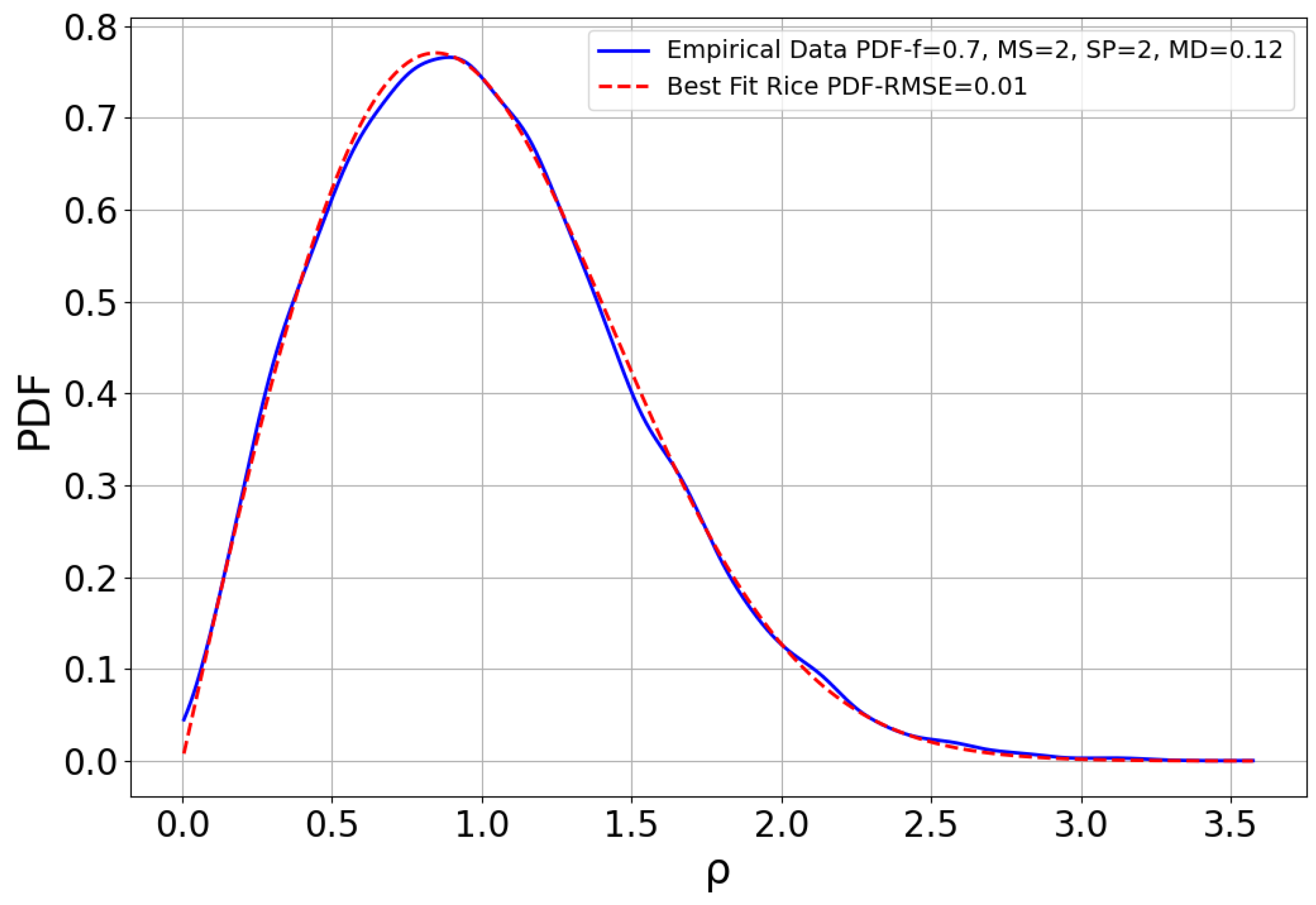
• Empirical PDF Construction: The PDF of the $\rho$ samples is extracted from the empirical data.
• Rice Distribution Fitting: The Rice distribution is fitted to the empirical PDF, and the corresponding K value is recorded to fill the database necessary to train and test the ML model.
• Dataset Compilation: The final dataset is compiled, containing columns for the features of each scenario (MS, SP, MD, and f) and the corresponding output K.

Figure 2 clearly shows that the empirical PDF is usually close to a Rice distribution, which also proves that the outcomes of RT simulations are physically sound.

3.5. Machine Learning

After the final dataset was obtained from the RT fast-fading analyses, it was divided into a training and a test set, with 80% of the data used for training the model and 20% reserved for testing.

The chosen ML model is based on the approach described in [7]. It consists of three different steps:

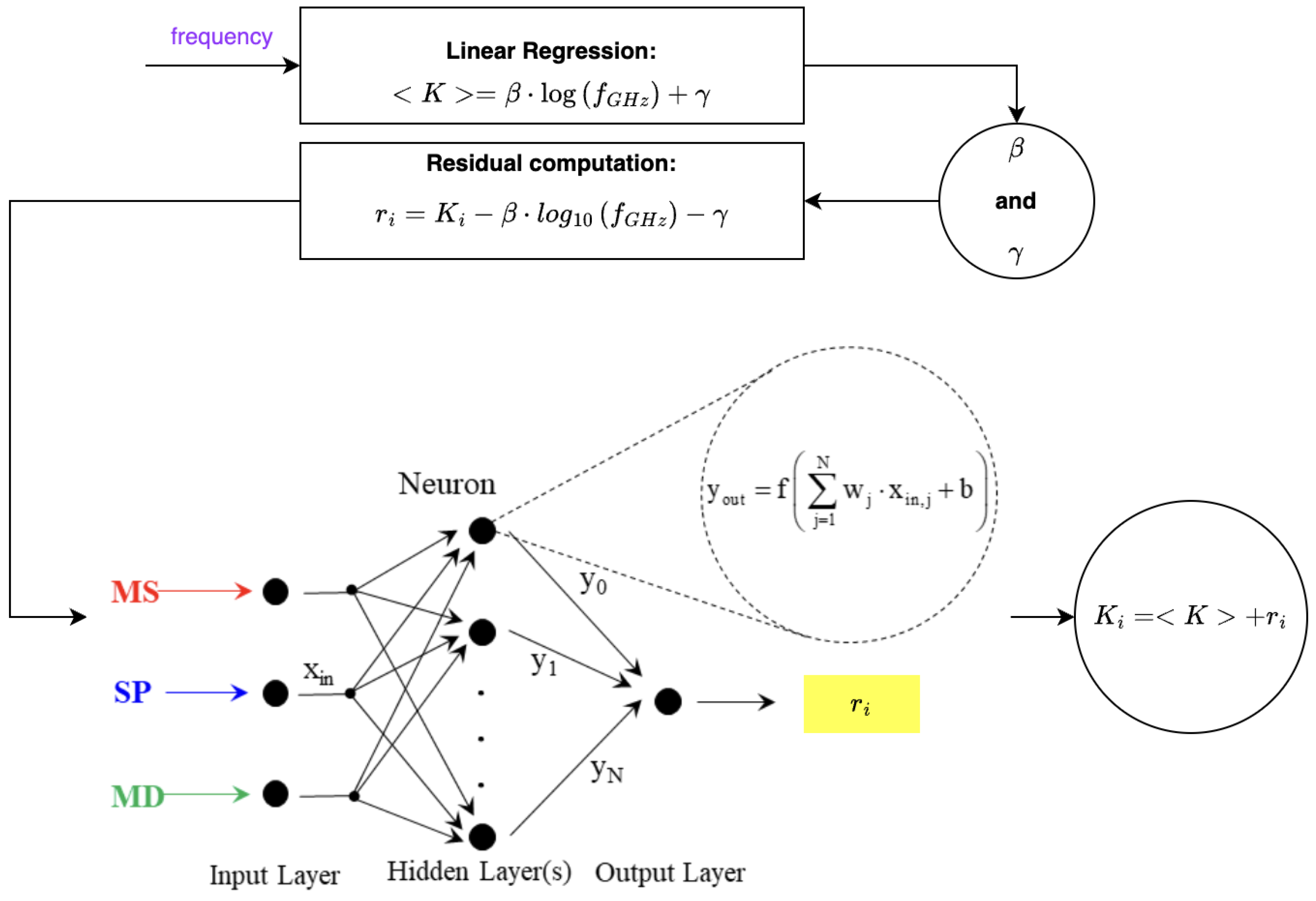
• A single linear regression is performed to estimate the frequency dependence of the Rice factor K. The regression model is defined as follows:

  $$<K>=\beta ·lo{g}_{10}\left(f_{GHz}\right)+\gamma ,$$

  (6)

  where $\beta$ and $\gamma$ are the regression coefficients. This step provides an initial estimate of K, capturing its average trend as a function of the logarithm of frequency. The coefficients are determined using the least squares method, minimizing the difference between the measured K values and the predicted trend.
• While the linear regression captures the overall frequency dependence, the actual values of $K_i$ deviate from the estimated trend due to environmental factors. The residuals $r_i$ quantify these deviations:

  $$r_i=K_i-\beta ·lo{g}_{10}\left(f_{GHz}\right)-\gamma ,\mathrm{i}=1,2,...,192.$$

  (7)
• A Multi-Layer Perceptron (MLP) is employed to model the residuals as a function of the environmental parameters MS, SP, and MD. The MLP consists of an input layer, hidden layers, and an output layer, with the following operations: The input layer receives the three geometrical features MS, SP, and MD. Hidden layers apply non-linear transformations using neurons, each performing the following:

  $$y_{out}=f\left(\sum _{j=1}^N{w}_j·x_{in,j}+b\right),$$

  (8)

  where $w_j$ are the trainable weights, b is the bias term, and $f\left(\right)$ is an activation function (e.g., ReLU). In the training process, the MLP is trained using backpropagation and gradient descent to minimize the error between the predicted residuals $\widehat{r_i}$ and the actual residuals $r_i$. In the output layer, the final estimate of the residual $\widehat{r_i}$ is produced. Finally, the corrected Rice factor is estimated by adding the predicted residual to the regression model:

  $${\widehat{K}}_i=\beta ·{log}_{10}\left(f_{GHz}\right)+\gamma +{\widehat{r}}_i.$$

  (9)

A summary of the proposed model is illustrated in Figure 3, which visually represents the three-step process.

Once the model is trained, its performance is evaluated on a separate test set to ensure its generalization capability. The test set consists of data points that were not used during training, allowing an unbiased assessment of the model’s predictive accuracy.

To quantify the prediction error, the Root Mean Squared Error (RMSE) is used as the performance metric. The RMSE measures the average magnitude of the residual errors between the predicted values $\widehat{K_i}$ and the actual values $K_i$, providing an indication of how well the model captures the variations in the Rice factor. It is defined as follows:

$$RMSE=\sqrt{{\displaystyle \frac{1}{N}}\sum _{i=1}^N{(K_i-{\widehat{K}}_i)}^2}.$$

(10)

4. Results and Discussion

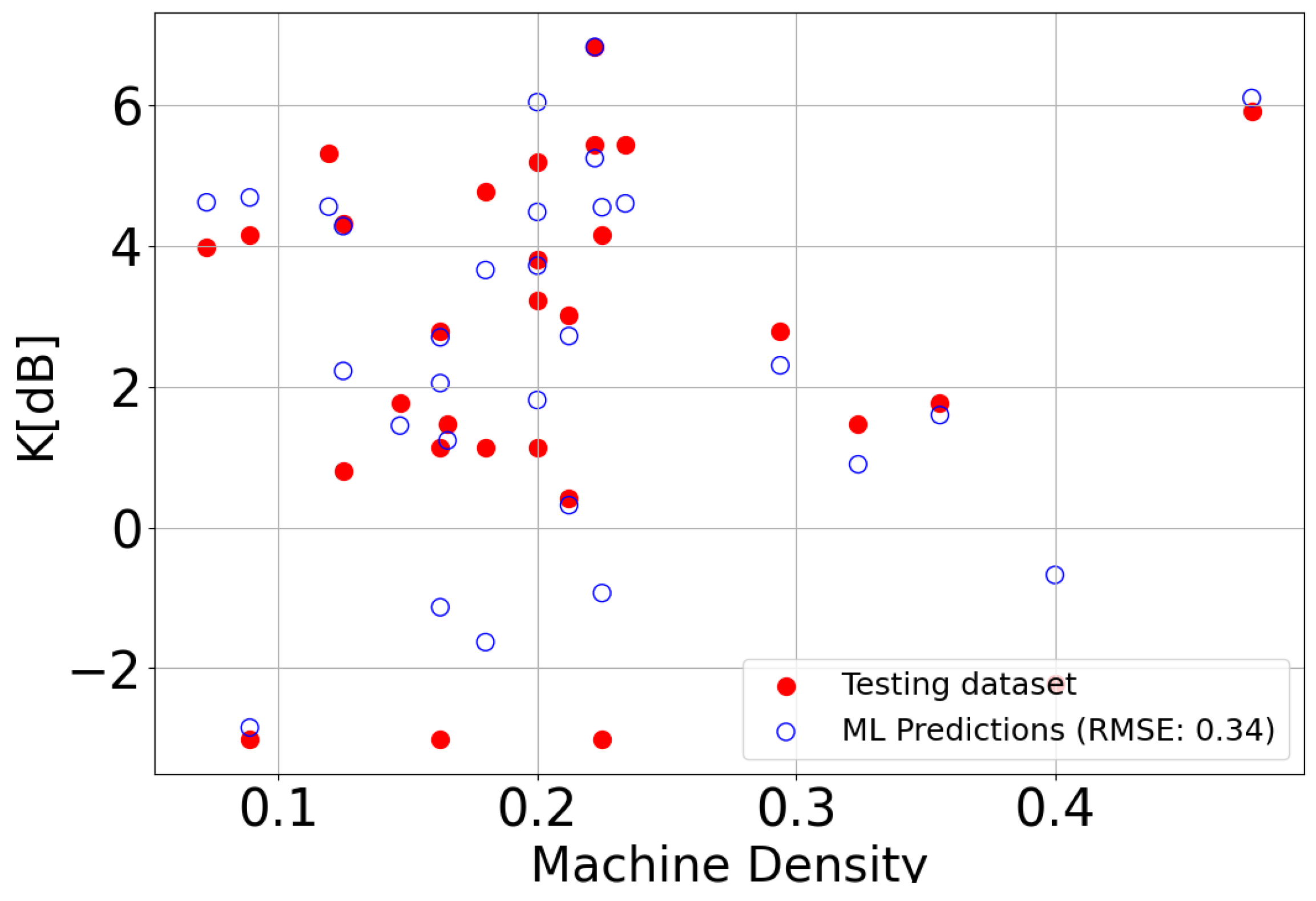
4.1. ML Model Evaluation

The model parameters, including the number of hidden nodes, learning rate, and activation function, were tuned to optimize performance.

Table 3. MLP model hyperparameters.

Parameter	Value
Hidden Layer Sizes	(8, 4)
Maximum Iterations	3000
Early Stopping	True
Learning Rate	0.001
Activation Function	ReLU
Solver	Adam

lists the main hyperparameters of the MLP model. The chosen configuration balances prediction accuracy and computational efficiency.

The selected MLP model, as shown in Table 3, consists of two hidden layers with 8 and 4 neurons, making it well-suited for the dataset size. The inclusion of early stopping ensures that training halts once no further improvement is observed, while the Adam optimizer facilitates efficient convergence. From a computational complexity perspective, let N denote the number of training instances (192), d the number of input features (3, corresponding to MS, SP, and MD), H the total number of neurons in hidden layers (8 + 4 = 12), and T the total number of training iterations. Each training iteration consists of a forward pass, where activations are computed, and a backward pass, where gradients are calculated and weights are updated. The per-instance complexity of a forward pass is $O(d·H)$, and the backward pass has the same order of complexity. Thus, for N instances, the total computational cost per iteration is $O(N·d·H)$. Over T training iterations, the total complexity becomes $O(T·N·d·H)$. Since the hidden layers contain a small number of neurons and early stopping prevents excessive iterations, the model remains computationally efficient while balancing accuracy and training speed. In practice, training is completed in just a few seconds, demonstrating its scalability for moderate-sized datasets.

The performance of the model is outlined in Figure 4, where the K values predicted by the ML model for the industrial layouts belonging to the test dataset are compared with the corresponding ground truth values returned by the RT simulations. A close agreement is achieved in most cases, as also confirmed by the corresponding RMSE reported in

Table 4. Performance of ML model and empirical formula.

Model	RMSE	Min K	Max K
ML Model	0.34	0	6.7
Empirical Formula	0.62

.

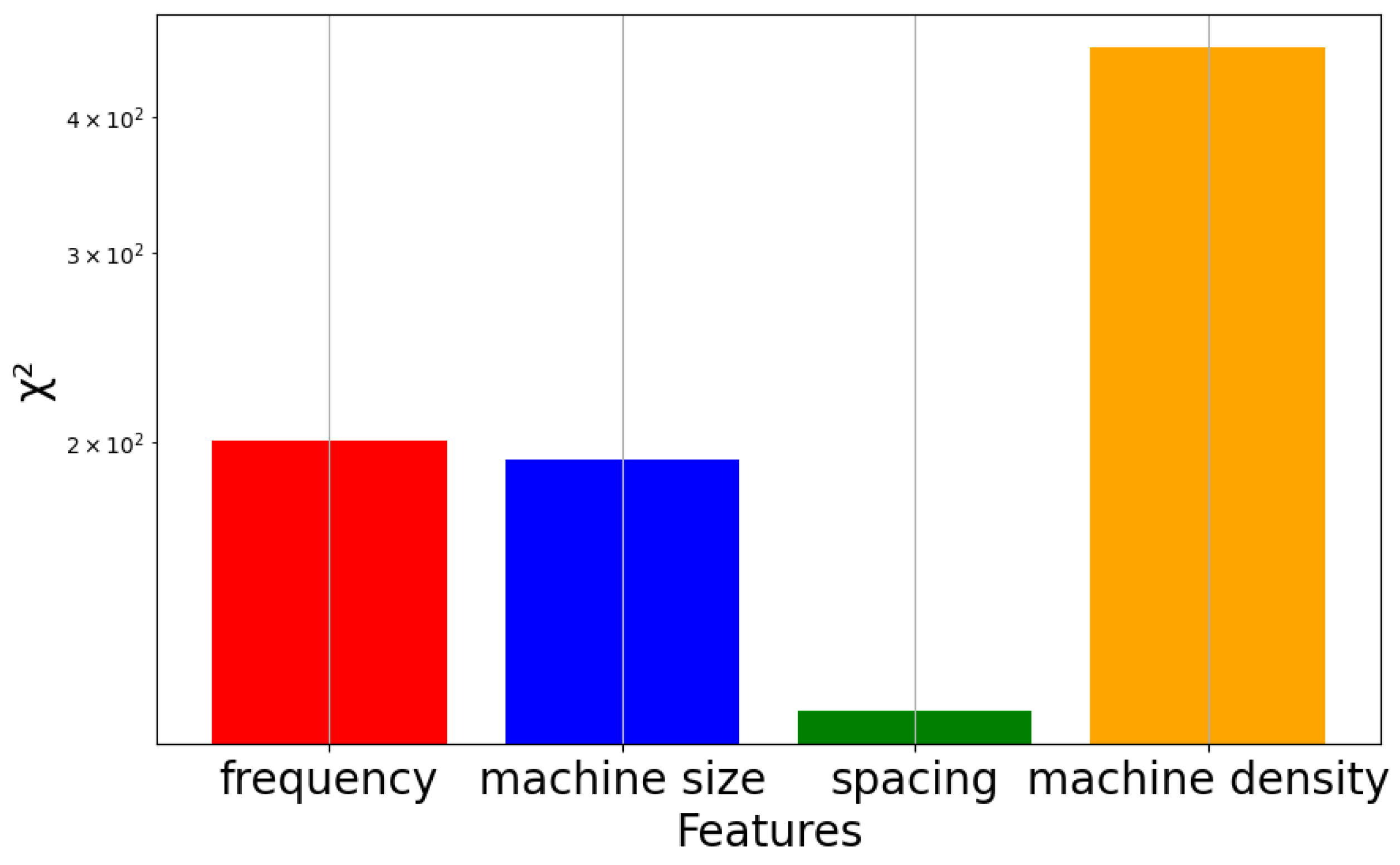
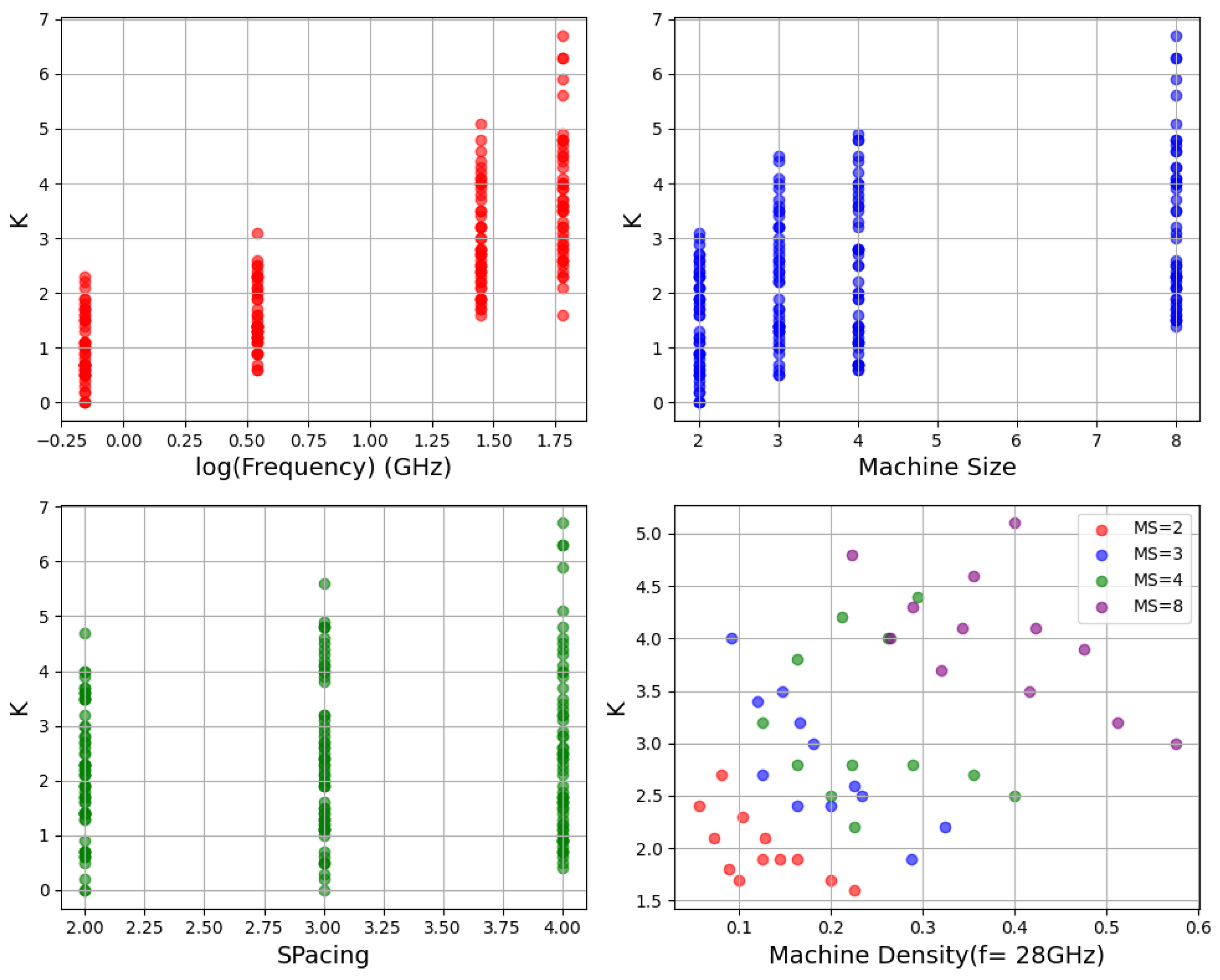
4.2. Feature Importance and Analysis

A preliminary analysis based on the Chi-square test was conducted on the collected dataset to investigate the features that mostly affect the K in industrial environments. As shown in Figure 5, machine density appears to be the most significant predictor of the K value, followed by frequency and machine size, with spacing showing negligible impact.

Figure 6 illustrates the relationship between the K factor and four different features: ${log}_{10}$(freq), machine size, spacing, and machine density. The trend suggests a general increase in K as ${log}_{10}$(freq), machine size, and spacing increase, indicating a positive correlation. In particular, K exhibits a linear-like dependency on these features, showing distinct clustered values at discrete feature levels. However, the relationship with machine density shows a different pattern. Since higher machine density implies more obstructions, K tends to decrease as machine density increases, which aligns with the expectation that more obstructions lead to lower K values. To better illustrate this, only the 28 GHz frequency case is considered, where K is plotted against machine density for different machine sizes. This approach clarifies the negative trend, further supported by the formula in Section 4.3, where the coefficient for machine density is negative. These observations reinforce the hypothesis that geometric and frequency-related features influence K, motivating the use of a predictive model like MLP to capture residual dependencies beyond simple regression.

4.3. Empirical Formula

In order to provide the reader with a ready-to-use, flexible model to predict the Rice factor in the industrial environment, the following simple linear expression is also proposed herein:

$$K=A+B·{log}_{10}\left(f_{\mathrm{GHz}}\right)+C·MS+D·MD.$$

(11)

The best values for the coefficients, i.e., corresponding to the lowest RMSE with respect to the ground truth values from RT, were computed through the least squares method, leading to values of $A=0.221$, $B=0.619$, $C=0.359$, $D=-2.0609$.

It is worth pointing out that the considered linear expression does not certainly represent the optimal formulation, as the true relationship between K and the input parameters included in Equation (11) is more complex than linear, as also stated in the introduction. This is the main reason why ML was relied on as a more reliable approach than fast-fading modeling. Nevertheless, the empirical formula turns out to be fairly accurate, in spite of its rough simplicity, as shown by the corresponding RMSE reported in Table 4.

It is worth noting that the procedure was performed for the Rice factor, given that the Rice distribution is widely used in the literature to investigate fast-fading samples. Similar approaches can be applied to other distributions, such as the Nakagami-m distribution.

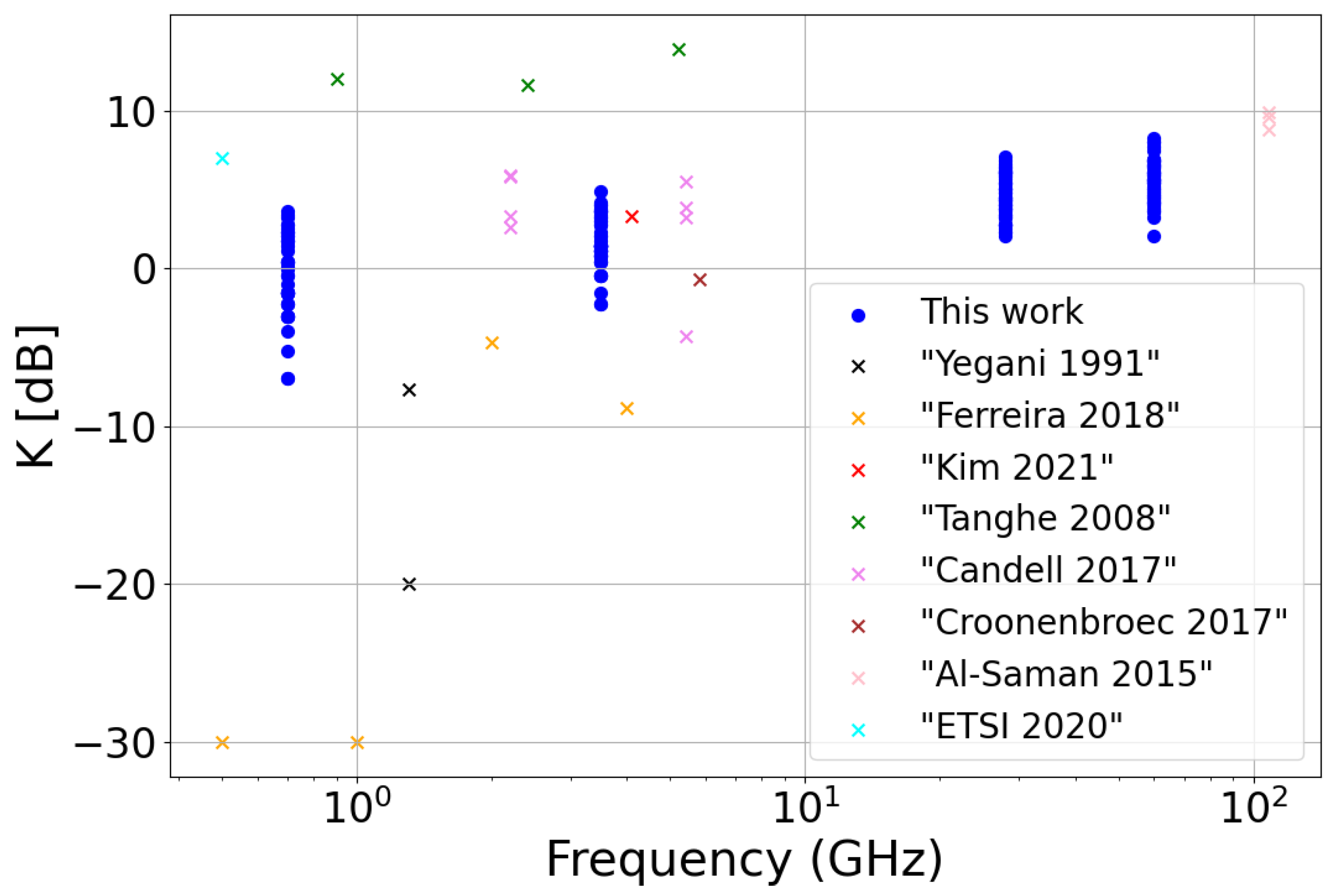
5. Comparison with the Literature

Figure 7 compares the Rice factor values achieved in this study with those collected from a literature survey. The blue dots come from the RT simulations carried out at the different frequencies on the considered 192 industrial layouts, whereas the crosses correspond to refs. [8,9,10,11,12,13,14]. Although these previous analyses concern industrial wireless propagation, they do not provide any detailed description of the considered industrial scenario, which means clear information about machine density, size, and spacing is never included. Nevertheless, the RT-based assessment is in general agreement with previous investigations. In addition to this agreement, the proposed approach offers greater flexibility, as it provides a relationship between the Rice factor and some geometrical parameters describing the industrial scenario, plus frequency, whereas other studies simply propose K values usually extracted from measurement campaigns, with no possibility of tuning.

6. Conclusions

In this work, Rice factor characterization in industrial environments was addressed by employing a machine learning approach including a simple linear regression and a neural network. Training and test data were obtained through RT simulations. Moreover, an empirical formula is proposed to estimate the Rice factor based on the communication frequency and the geometry of the environment. Satisfactory performance of both the machine learning model and the empirical formula was achieved. Overall, the results are in general agreement with previous investigations and existing models and also highlight some clear trends between the Rice factor and parameters like communication frequency and machine density and size. Specifically, the Rice factor increases at higher frequency and larger machine size, while it decreases at greater machine density.

References

1. Vitturi, S.; Tramarin, F.; Seno, L. Industrial Wireless Networks: The Significance of Timeliness in Communication Systems. IEEE Ind. Electron. Mag. 2013, 7, 40–51. [Google Scholar] [CrossRef]
2. Candell, R.; Kashef, M.; Perez-Ramirez, J.; Conchas, J. An IEEE Standard for Industrial Wireless Performance Evaluation. IEEE Internet Things Mag. 2023, 6, 82–88. [Google Scholar]
3. Zurawski, R. Industrial Communication Systems; CRC Press: Boca Raton, FL, USA, 2005. [Google Scholar]
4. Cheffena, M. Industrial Wireless Communications over the Millimeter Wave Spectrum: Opportunities and Challenges. IEEE Commun. Mag. 2016, 54, 66–72. [Google Scholar] [CrossRef]
5. Bertoni, H.L. Radio Propagation for Modern Wireless Systems; Prentice Hall Professional Technical Reference: Upper Saddle River, NJ, USA, 1999. [Google Scholar]
6. Saunders, S.R.; Zavala, A.A. Antennas and Propagation for Wireless Communication Systems; Prentice Hall Professional Technical Reference: Upper Saddle River, NJ, USA, 1999. [Google Scholar]
7. Zadeh, M.H.; Barbiroli, M.; Fuschini, F. A Machine Learning Approach to Wireless Propagation Modeling in Industrial Environment. IEEE Open J. Antennas Propag. 2024, 5, 727–738. [Google Scholar] [CrossRef]
8. Yegani, P.; McGillem, C. Industrial Wireless Systems: Radio Propagation Measurements. IEEE Trans. Comm. 1991, 39, 10. [Google Scholar]
9. Ferreira, M.; Ambroziak, S.; Cardoso, F.; Sadowski, J.; Correia, L. Fading Modeling in Maritime Container Terminal Environments. IEEE Trans. Veh. Tech. 2018, 67, 10. [Google Scholar] [CrossRef]
10. Kim, J.; Kim, C.; Hong, J.Y.; Lim, J.S.; Chong, Y.J. Propagation Characteristics of an Industrial Environment Channel at 4.1 GHz. In Proceedings of the 2021 International Conference on Information and Communication Technology Convergence (ICTC), Jeju Island, Republic of Korea, 20–22 October 2021. [Google Scholar]
11. Tanghe, E.; Joseph, W.; Verloock, L.; Martens, L.; Capoen, H.; Herwegen, K.V.; Vantomme, W. The industrial indoor channel: Large-scale and temporal fading at 900, 2400, and 5200 MHz. IEEE Trans. Wirel. Comm. 2008, 7, 7. [Google Scholar]
12. Candell, R.; Remley, C.; Quimby, J.; Novotny, D.; Curtin, A.; Papazian, P.; Koepke, J.D.G.; Hany, M. A Statistical Model for the Factory Radio Channel; Technical Report, NIST Technical Note; National Institute of Standards and Technology: Gaithersburg, MD, USA, 2017. [Google Scholar]
13. Croonenbroeck, R.; Underberg, L.; Wulf, A.; Kays, R. Measurements for the development of an enhanced model for wireless channels in industrial environments. In Proceedings of the 2017 IEEE 13th International Conference on Wireless and Mobile Computing, Networking and Communications (WiMob), Rome, Italy, 9–11 October 2017. [Google Scholar]
14. Al-Saman, A.; Mohamed, M.; Cheffena, M.; Moldsvor, A. Wideband Channel Characterization for 6G Networks in Industrial Environments. Sensors 2021, 21, 2015. [Google Scholar] [CrossRef] [PubMed]
15. ETSI TR 138 901; Study on Channel Model for Frequencies from 0.5 to 100 GHz. Technical Report; ETSI: Sophia Antipolis, France, 2020.
16. Fuschini, F.; Vitucci, E.; Barbiroli, M.; Falciasecca, G.; Degli-Esposti, V. Ray tracing propagation modeling for future small-cell and indoor applications: A review of current techniques. Radio Sci. 2015, 50, 469–485. [Google Scholar] [CrossRef]
Figure 1. Example of industrial scenario: MS = 2, SP = 4, T = 0.5, MD = 0.05. Boxes, red dots, and blue dots represent the machines, receivers, and transmitter, respectively.
Electronics 14 01378 g001
Figure 2. An example of a best-fit Rice distribution.
Electronics 14 01378 g002
Figure 3. Diagram of the model.
Electronics 14 01378 g003
Figure 4. Comparison between ML prediction and RT ground truth (test set).
Electronics 14 01378 g004
Figure 5. Feature importance.
Electronics 14 01378 g005
Figure 6. Feature analysis.
Electronics 14 01378 g006
Figure 7. Comparison with the literature. Yegani 1991 [8], Ferreira 2018 [9], Kim 2021 [10], Tanghe 2008 [11], Candell 2017 [12], Croonenbroec 2017 [13], Al-Salman 2015 [14], ETSI 2020 [15].
Electronics 14 01378 g007