1. Introduction
As one of the most widely used sensors in Autonomous Driving (AD), Light Detection And Ranging (LiDAR) sensors provide excellent spatial resolution in the form of 3D point clouds. Compared to other sensors, LiDAR systems actively illuminate the scene, producing enough rich details to detect obstacles solely on 3D point clouds [
1]. Motorized optomechanically scanning LiDAR is the most common, with single rotation axis or even dual-axis systems [
2]. However, the natural issues of the scanning process include large gaps, narrow vertical view, slow scene updating and limited placement options on the vehicle [
3]. Additionally, despite their active illumination, LiDAR systems remain susceptible to challenging environmental conditions like sunlight, fog or rain, which can introduce noise.
To address these challenges, non-mechanical flash LiDAR and ToF cameras are emerging as compelling alternatives [
4]. Unlike mechanically scanning LiDARs, non-mechanical sensors have no moving actuators or mirrors, which not only improves their durability but also enables more versatile placement around larger vehicles, such as buses or trucks, where scanning coverage and mounting flexibility are crucial [
5]. However, implementing a distributed sensor system introduces significant design challenges, including the need for synchronous point cloud registration, increased complexity in in-vehicle software architecture, and the development of advanced computer vision algorithms for effective scene analysis, among other issues.
Point cloud registration from multiple sensors involves aligning and merging data from different partial views of the environment into a unified 3D model. The latest advancements employ feature-based matching and registration, identifying distinct geometrical features in overlapping regions of the point clouds [
6]. The resulting surround depth information is critical for many computer vision and scene analysis applications, including 3D object detection [
7]. While Artificial Neural Networks (ANNs) are effective in learning complex spatial features in point cloud data, they can be computationally expensive, especially when deployed in real-time environments where energy efficiency, processing speed, and latency are critical factors, including applications such as autonomous vehicles and robotics [
8].
Meanwhile, SNNs are attracting attention for energy-efficient object detection and decision-making [
9,
10]. Their inherent ability to operate asynchronously aligns well with real-time object detection, where incoming data streams are often irregular, as seen with point cloud data from LiDAR and ToF sensors.
Altogether, the autonomous vehicle is an intricate software-guided application that uses computer vision, sensors, data fusion, information communication, high-performance computing, artificial intelligence, real-time control, and other technologies [
11]. Moreover, machine vision, which is the key entry point of AD software, must address safety-aware design principles supporting systems ranging from Level 2+ to Level 5 fully autonomous driving, as classified by the Society of Automotive Engineers (SAE) J3016 standard [
12].
The aim of this work is to provide a coherent AD-suitable perception system architecture based on distributed non-scanning ToF sensors. Unlike many existing long-range, low-resolution scanning LiDAR systems, we focus on a close-range, high-resolution, and flexibly mountable sensor system designed for blind zone monitoring.
The remainder of the paper is structured as follows.
Section 2 details the key topics discussed in the introduction, highlighting technical aspects ranging from safety to sensor working principles and algorithms.
Section 3 describes the overall system architecture and essential implementation details.
Section 4 introduces the experimental setup and provides result analysis for the system’s performance, point cloud registration, and object detection. Finally,
Section 6 summarizes the conclusions.
2. Literature Review
2.1. Assisted and Automated Driving
AD systems must comply with a set of challenges, including design complexity, safety mechanisms, evolving standards, cyber-security, etc. The impactful ISO26262 standard [
13] documents these safety aspects and defines the Automotive Safety Integrity Levels (ASILs) by specifying requirements for the development process and consecutive safety measures. However, achieving a true self-driving functionality, which conforms to the fourth and fifth levels of driving automation [
12], still requires research at the component and system levels. Furthermore, it requires user acceptance, for which the Advanced Driver-Assistance System (ADAS) is a natural gateway.
The stringent safety requirements conflict with the experimental nature and goals of the innovation process. For instance, the complexity of automotive electronic and electrical systems compelled the industry to join forces and establish the Automotive Open System Architecture (AUTOSAR) initiative [
14]. AUTOSAR strives to simplify software management while improving its flexibility, scalability, quality and integration. It structures software similarly to an operating system: application (platform independent), basic software (essentially platform implementation) and runtime environment (standardized interface between application and basic software). Notably, AUTOSAR is a relatively low-level industry standard.
Multiple frameworks and approaches are used for prototyping AD systems. Among the most popular are the Robot Operating System (ROS) [
15], which ensures software reusability with a universal communication mechanism. Consequently, ROS2 has significantly improved communication characteristics [
16] and an impending approach for real-time systems. ROS is also the basis for the world’s leading open-source autonomous driving project—Autoware [
17].
Notably, industry-driven all-encapsulating AD solutions have emerged as part of the attempt to capitalize on the growing market, including solutions from major vendors like Intel (Mobileye, full-stack solution based on EyeQ SoC), NXP (BlueBox extensible development platform), NVIDIA (GPU-centric Drive platform) and others. These hardware-centric solutions present an ever-growing ecosystem with evolving software and features. However, a significant drawback, especially for research purposes, is the software’s proprietary nature and the eventual lack of support.
2.2. Photonic Depth Imaging Principles
Three-dimensional data are important for many robotics, safety, and other applications, and have led to the development of several different approaches for depth and 3D structure estimation.
Classic stereoscopy approaches employ multiple regular cameras observing the same scene, representing a cost-effective solution. Depth information is obtained by matching and triangulating homologous points across stereo image frames. Feature-based matching algorithms extract simple geometrical elements, such as lines and corners, and perform matching between sets of such features. In contrast, correlation-based algorithms match directly between image fragments, which results in much denser disparity maps but is more computationally intensive and sensitive to intensity variations. The performance of both methods depends on the scene and is significantly reduced in the absence of features or textures. As a result, the disparity maps become sparser in such regions. Active stereoscopy introduces additional features by projecting a pattern onto the scene [
18].
Structured light depth sensors represent another approach to optical triangulation. A simple structured light-ranging system consists of one camera and a laser source. The laser beam is angled in such a way that the position of the projected dot, as observed by the camera, depends on the distance to the object it is projected on. Structured light camera sensors range the entire scene by projecting a two-dimensional pattern. To ensure unambiguous correspondences, the pattern either varies in colour, changes over time, or is spatially unique [
18].
In contrast with triangulation, Time-of-Flight approaches allow for more direct distance measurement, which offers higher accuracy and is not dependent on the sensor’s spatial resolution, which greatly improves precision consistency across the distance range. A simple ToF ranging system consists of two components—a laser and a photodetector. To measure the distance to a certain object, a short laser pulse is emitted, which then travels to the object, is reflected, travels back, and finally is observed by the photodetector. Due to the finite speed of light propagation, a short delay between the emitted and observed pulses is present, which is equal to the round trip time of the laser pulse. The distance
d to the object of interest can then be calculated as
, where
is the measured time delay and
is the speed of light [
19].
In order to aid the co-existence of ToF sensors with human agents, the emitted light is outside of the range perceived by humans. Infrared wavelengths of 850 nm and 940 nm are the ones commonly used. 940 nm roughly corresponds to a dip in the solar irradiance spectrum. Therefore, sensors using this wavelength are intrinsically more robust in outdoor environments. On the other hand, just as the dip is caused by light absorption by water vapour, performance in humid conditions is also degraded. Another advantage of the 850 nm wavelength is the greater efficiency of the photodetectors. Thus, 850 nm ToF sensors have the potential to perform better even in sunny conditions but require additional attention to be paid to the ambient light rejection solutions [
20].
To range beyond just a single point, LiDAR sensors introduce a third component—the scanner—which diverts the laser to scan it across the whole scene. Automotive applications usually employ separate scanners for two axes, although in some use cases, even one scanning axis might be sufficient. Depending on the scanning method, LiDARs are classified as mechanical, solid-state, and quasi-solid-state. In mechanical sensors, scanning is performed by moving the entire optical assembly. In quasi-solid-state sensors, most of the components remain stationary and only the laser beam is deflected, which is achieved using rotary mirrors or MEMS micromirrors. Finally, solid-state sensors have no moving parts at all, which can be achieved by using an optical phased array to form the scanning beam [
5,
19].
Another way of implementing a solid-state optical ranging sensor is to forgo sequential scanning altogether and instead illuminate the entire scene at the same time. The reflected light is then collected by an array of photodetectors, much like in a regular camera. This type of sensor is commonly called the Time-of-Flight camera. It is also sometimes called the Time-of-Flight sensor, which is somewhat confusing, since LiDARs also operate on the Time-of-Flight principle. To add to the confusion, some manufacturers also use the term Flash LiDAR to refer to essentially the same operating principle, although certain solutions have claimed to use multiple focused laser beams to individually illuminate areas corresponding to each pixel of the detector array, thus offering improved efficiency [
20]. To use the most common terminology, in this paper, the term “LiDAR” refers exclusively to scanning ranging systems, while the terms “ToF camera” and “ToF sensor” are used for solid-state sensors with full-scene illumination.
Scanning LiDAR is currently the most prevalent depth-sensing technology in assisted and autonomous driving applications. It is featured in most of the contemporary autonomous driving solutions, both those that are commercially available and those that are under development. In the DARPA Grand Challenge and subsequent events—competitions for fully autonomous ground vehicles—almost all of the vehicles that made it to the finish line were using at least one LiDAR [
19]. ToF cameras offer several advantages over scanning LiDAR sensors, which all stem from the simultaneous acquisition of the entire scene. Their mechanical construction is much simpler, which reduces the cost and increases robustness. Using indirect ToF measurement techniques, pixel size can be shrunk down, increasing pixel density and sensor resolution. They do not suffer from motion blur caused by sequential scanning, although they are not completely blur-free, as a single depth frame usually requires several sub-frames [
21]. ToF cameras also offer much greater freedom of sensor placement due to the reduced size and wide field of view that can be achieved depending on the chosen lens. However, there are some additional considerations. Most importantly, the sensor should not have any objects in close proximity due to the distortions caused by strong reflected light [
21].
In addition to LiDAR and ToF cameras, other sensing modalities such as ultrasonic sensors have been explored for perception in autonomous vehicles. Ultrasonic rangefinders, commonly used for close-range obstacle detection, have been proposed as complementary systems to overcome certain limitations of LiDAR, particularly when it comes to detecting small or low-reflectivity objects at close distances [
22]. Furthermore, sensor fusion techniques combining LiDAR with ultrasonic sensors and wheel speed encoders have been investigated to improve the robustness of mobile robot navigation [
23]. These hybrid approaches leverage the strengths of different sensing technologies to reduce measurement errors.
2.3. Surround-View Visual Awareness
Human perception mainly processes and enhances sensory information, enabling individuals to sense, orient, and react quickly, accurately, and efficiently. However, certain constraints limit human perceptual capacity when driving, posing significant risks to the vehicle driver and other road users [
24]. At high speeds, drivers experience a narrowed field of vision, known as “tunnel vision”, which limits peripheral awareness, combined with additional distractions on the road and unpredictable actions from other drivers and pedestrians, and the physical limitations of the vehicles worsen the circumstances, leaving critical areas, particularly vehicle blind spots, partially or entirely out of the driver’s view. This is especially hazardous for drivers of large vehicles, such as trucks, for which extensive blind zones can obscure nearby road users [
25].
ADAS are developed to handle the limitations mentioned above by enriching driver awareness and safety through data fusion from multiple sources, including automotive imaging, LiDAR, radar, computer vision, and in-cabin notifications, providing drivers with critical situational information and, depending on the system’s level, potentially taking partial control of the vehicle to prevent or mitigate potential threats [
26].
A surround view perception system functions as an informational assistance at SAE Level 0 and as a critical cornerstone at SAE Level 2+, providing real-time environmental representation around the vehicle through either a LiDAR or a combined set of 3D ToF cameras [
27], as shown in
Figure 1.
Point Cloud Registration
Each ToF camera in a surround view system operates within its coordinate system, which means that a single spatial point appears at different relative distances from the perspective of each camera, which complicates spatial perception for the driver, as shown in
Figure 2a, where the blue and yellow points represent the same physical points observed from different perspectives that can be unified using a registration pipeline such as Deep Global Registration (DGR) [
28,
29,
30], where all points in both clouds are characterized by descriptive features which are then matched to identify common correspondences, between the pointclouds, that can be used to estimate the optimal transformation matrix to align one pointcloud with another [
31], as shown in
Figure 2b.
2.4. Environmental Representation
Regardless of perception type, there are multiple ways to represent the perceived environment for both the ADAS and the user. The environment representation types can be classified into several groups, namely raw point [
32,
33], feature-based [
34,
35,
36], grid map [
37,
38,
39,
40], and topological [
41] representations.
Each representation has its strengths and drawbacks, and no single solution fits all use cases [
27]. Raw point representation includes all measurement points (of depth-based sensors) but can have large storage requirements. Additionally, these points are susceptible to noise without filtering. Semantic information can be included in raw point representation (e.g., point colour) [
42,
43] to represent object types, which can improve readability for human operators. Point representations are a commonly used input for modern object detection algorithms, but can be harder to interpret for humans due to 3D information usually being displayed in 2D. Combining points into larger, more meaningful objects like planes, lines, or other distinct features can further increase readability for humans, which enables the feature-based representations to be more understandable to humans. However, these representations require more complex algorithms for use in path-finding or object detection. Topological representations further abstract the environment by combining sections of the environment into nodes (and storing the relation between these nodes). This approach is useful for large-scale path planning but loses detailed information on nearby road obstacles like other traffic participants. Grid maps discretize the environment into small sections—cells—that contain information about the state of the environment in that section. Grid representation can be used for object detection due to its voxelizing nature and is especially suited for obstacle representation. The cells of the grid map can contain information on cells’ affiliation with a certain type of object (semantics), but cells most commonly represent the state of the environment in terms of occupancy—free, occupied, or unknown. Hence, the name of the most widespread grid map type is the OGM. This representation is straightforward and understandable for a human operator in an ADAS visualization and is commonly used for path-planning algorithms.
The mechanics behind OGM generation are straightforward—store the state of a section of the world in a grid structure, which can be displayed to the user and/or used to avoid obstacles by ADAS or the user directly. The initial approach proposed in [
37] stores the value of occupancy as a probability
p from 0 to 1, where 0 stands for certainly free and 1—certainly occupied. However, absolute certainty is rare; therefore, certain thresholds can be introduced, e.g., 0 ≤
p ≤ 0.2 is considered free and 0.8 ≤
p ≤ 1 is considered occupied. The range in between these states is marked as unknown. To calculate the states of the cells, generally, binary Bayes filter [
44] is used with the cell initial value of 0.5 and the use of an inverse sensor model [
37]. There have been alternative approaches that implement Random Finite Sets [
45,
46] to estimate the occupancy probability (
p), but the main principle remains the same: to increase the occupancy of cells where measurements are recorded. Free space, on the other hand, is modelled on the assumption that space up to the measurement is free. Otherwise, the measurement would have been recorded earlier. Due to inherently noisy sensors, both free and occupied space is estimated using either inverse or forward sensor models, but due to complexity issues, inverse sensor models are more common [
44]. For ToF-based sensors (LiDAR, RADAR, etc.), ray tracing can be used to model each measurement point—a ray from the origin of the sensor to each measurement point in the point cloud is produced. Along each ray, tracing can be performed, where all cells that do not contain a measurement or are crossed by a ray have their
p decreased, while all cells at the ends of rays have their
p increased.
In this work, we adapt OGM representation for environment representation based on multiple ToF sensors. The cell occupancy probability is updated with the aforementioned binary Bayes filter for both occupied and free cells. ToF sensors are modelled similarly to LiDAR sensors, with an inverse sensor model. The resulting representation can then be used to notify vehicle users of obstacles in their blind zones as part of ADAS or for re-planning a path in case of obstacles for AD vehicles.
2.5. Current Advances in Deep Learning for LiDAR and ToF Sensors
Data-driven deep learning (DL) models, particularly convolutional neural networks (CNNs) and, more recently, graph neural networks (GNN) and transformer-based architectures, have been employed to extract complex features from sparse point clouds with high accuracy [
1,
47]. Recently, autonomous driving has led to significant advancements in 3D object detection, supported by numerous publicly available scanning LiDAR datasets such as KITTI [
48], nuScenes [
49], and Waymo [
50]. In contrast, datasets for solid-state flash LiDAR and non-scanning ToF sensors in the automotive domain are far less common, with notable examples including PixSet [
51], PandaSet [
52] and SimoSet [
53].
Despite the limited availability of solid-state flash LiDAR and ToF datasets, many existing 3D object detection methods designed for traditional LiDAR can still be adapted to these sensor types. Techniques such as point cloud-based deep learning models, including PointPillars [
54] and PV-RCNN [
55], can be retrained on ToF or flash LiDAR data with minimal modifications. For instance, PV-RCNN was successfully retrained on the PandaSet non-scanning LiDAR dataset [
52]. Compared to state-of-the-art LiDAR systems, the proposed non-scanning ToF approach offers key advantages in terms of latency, scalability, and simpler integration than mechanical LiDAR, making it better suited for distributed perception systems.
Existing deep neural networks achieve supreme accuracy, but converting point cloud data into structured formats often results in significant data explosion. Additionally, conventional DNN computations rely on dense multiply-accumulate (MAC) operations, which are poorly suited for processing the inherently sparse ToF data. In contrast, human vision-inspired neuromorphic computing captures, transmits, and processes stereo visual information in discrete spikes, maintaining low data volumes [
56]. Inspired by this efficient approach, prior research on 3D SNN object detectors [
57,
58] and segmentation [
59] has utilized the KITTI Vision benchmark dataset with scanning LiDAR to explore more data-efficient solutions. Moreover, recent advancements in direct-coupled solutions [
56] are integrating neuromorphic computing with indirect Time-of-Flight (iToF) SPAD imaging sensors and direct Time-of-Flight (dToF) [
60]. These early prototypes demonstrate 3D object classification and detection using efficient integrate-and-fire (IF) neurons within a five-layer spiking convolutional neural network (SCNN). Although promising, complex 3D feature extraction requires deeper networks with more advanced adaptive-threshold leaky integrate-and-fire (LIF) neurons to handle diminishing activity in deep hidden layers and achieve higher accuracy [
61].
In this work, we build on previous research [
57,
62] by adapting the described framework for 3D object detection using ToF data. This approach incorporates adaptive LIF neurons, which are crucial for maintaining stable network activity throughout deeper layers, thereby preventing the diminishing activity often observed in conventional SNN architectures and enabling high accuracy in object detection tasks, specifically on ToF sensor data. This approach extends the application of neuromorphic techniques to ToF-based perception systems, offering a more accurate SNN for reliable and power efficient AD software architectures.
3. System Architecture and Implementation
3.1. Software Architecture
Enabling topological experimentation and simultaneously addressing the requirements of safety criticality and real-time control presents a substantial challenge. Although the popular ROS framework [
15] provides topological flexibility, i.e., a blackboard software design pattern, it does not satisfy any real-time requirements or process synchronization and also demands significant resources [
63], hindering the deployment of the perception system. The limitations of ROS facilitated workarounds and an eventual ground-up redesign, i.e., ROS2 [
16]. ROS2 incorporates major advancements, including improved communications, extended support for different operating systems, more coherent implementation, and better support for embedded systems. However, both frameworks are quite complex, with a relatively large codebase, spawning at least five threads per process node (except the master node in ROS1) [
63].
The perception system adopts a custom non-ROS-based approach, addressing the real-time performance requirements while providing fine-grained control and simplicity. The strategy is based on the following in-house low-level system architecture implementation frameworks.
compage [
64] is a framework for implementing component-based system architecture. The framework provides a means of “registering” standardized software components, which can be instantiated and configured via simple configuration files (no re-compilation necessary). The framework is efficient, has a lightweight codebase with minimal dependencies, and is compatible with C and C++.
icom [
65] is a complementary framework that provides abstract routines for the implementation of different Inter-Process Communication (IPC) techniques. icom enables a set of features, including non-invasive switching between different underlying communication mechanisms, zero-copy communication (currently supported only for multithreaded, single-process scenarios), and acknowledgments.
rtclm [
66] is a framework for real-time control-loop monitoring. The tool facilitates the aggregation of performance metrics for software loops in real-time control systems. The code inside these loops (embedded within the software components) emits minimalistic packages over a UDP communications protocol aggregated and stored by a server, often deployed on a separate machine to minimize interference. The collected performance metrics are available via a shared memory IPC mechanism, which is usable for real-time visualization, fault monitoring and alarm generation.
Figure 3 illustrates the overall software architecture of the proposed perception system. Every node represents a compage component, while intra-process communication is implemented using icom. The whole system (i.e., parameters, number and type of components, communication) can be configured using a simple .ini file. Here, frame grabbers receive data from different ToF sensor camera types. These nodes can be substituted with “fake” camera components that replay pre-recorded data for simulation and testing. Further, each 3D point cloud is processed separately using spatial transformation nodes. Transformed 3D data are further registered into a single-coordinate system while executing a runtime registration fidelity check. If the camera configuration has changed, the runtime calibration node attempts to calculate a new configuration for the transformations. Finally, the registered data are provided to conventional (CNN) and modern (SNN) inference nodes and an environment representation block, which converts 3D data into a grid map handoff for further collision avoidance and path-planning algorithms.
The modular and configurable software architecture enables external connections anywhere between the different nodes using TCP/IP-based communication. Nonetheless, the system generates multiple streams of data.
Joined (registered) 3D point cloud—can be used for an intuitive display of the vehicle’s surroundings. In our setup, this information directly streams into the GUI.
Per-frame list of detected objects—can be used to enhance the surrounding display and implement safety-critical functionalities. Notably, if the inference server is deployed on a computationally weaker machine, frames may be dropped out.
Two-dimensional Occupancy Grid Map—provides a 2D representation of the surrounding environment. It can be used for safety-critical functionalities and by path-planning algorithms.
System’s component execution monitoring information—data characterizing the system’s node performance, which is provided via a shared memory mechanism. The information can be used for overall performance monitoring and fault detection. For example, it is possible to detect component performance degradation and, consequentially, detect faults.
3.2. Synchronous Triggering and Frame Grabbing
Since ToF sensors are active devices that provide their own scene illumination, simultaneous operation of multiple sensors in the same area is likely to cause interference. Manufacturers of both sensors used in the system have taken different steps to mitigate this issue. Monstar cameras employ Spread Spectrum Clock (SSC) technology, which continuously shifts the modulation frequencies over time, thus minimizing the probability of several sensors that share the same frequency [
67]. Blaze cameras are synchronized using the Precision Time Protocol (PTP), and can operate in either interleaved or consecutive acquisition modes. In the interleaved mode, a slight acquisition delay is inserted for one of the sensors so that only one sensor is illuminating the scene at any given time. This mode allows for simultaneous operation but only supports up to two sensors. Alternatively, in the consecutive mode, each sensor begins acquisition only after the previous one has completed its cycle. This way, there is no limit on the number of sensors at the cost of reduced frame rate [
68]. If the sensors are not in the same network, it is also possible to assign each sensor to one of the seven frequency channels that do not interfere with each other [
69].
To achieve seamless stitching of individual point clouds, simultaneous data acquisition between the sensors must be ensured. Sensor synchronization can be achieved using the external trigger input, and both of the sensors used here provide such a capability. As previously described, simultaneous operation of active sensors can be non-trivial and prone to interference. Interference techniques vary between manufacturers, may depend on the number of cameras, and may not perform equally well in all conditions. Some of the issues encountered during testing are further described in
Section 4.1. Evidently, truly synchronous acquisition may not always be achievable; nevertheless, the stitching results can still be enhanced by improving acquisition consistency.
The triggering system providing the necessary flexibility, implemented in programmable logic to ensure consistent deterministic behavior, is shown in
Figure 4. The black arrows represent the flow of the trigger signal, which starts at the pulse generator. A set of delay units offset the trigger pulse by different period for each of the cameras, thus allowing a precisely controlled simultaneous or staggered sensor acquisition. Pulse shapers are inserted after the delay units to ensure the necessary trigger pulse width. All of the parameters are adjustable within the software through the configuration interface to allow users to choose the desired frame rate and set the delay for a particular sensor family. The configuration interface, drawn in purple, consists of configuration registers containing the variables used by individual components and configuration logic to make the registers externally accessible through a specific interface. In this system, a USB interface was used.
3.3. Unified Surround-View Point Cloud
The presented system uses ToF cameras positioned in a circular arrangement in clockwise or counterclockwise order, with overlapping fields of view between adjacent cameras to achieve surround-view spatial coverage of the environment. The layout can be modeled as a directed graph as shown in
Figure 5, where the nodes represent individual cameras, each working within a local coordinate system, and the edges encode the rigid transformations required to align neighboring pointcloud pairs.
Raw point clouds captured by the ToF cameras undergo a multi-stage preprocessing pipeline to improve the data quality and computational efficiency. For each pair of adjacent point clouds, the depth range is constrained to the minimum value observed between the two clouds, eliminating distant points that fall outside the overlapping region of interest, focusing computational resources on relevant spatial features, and minimizing ambiguities during feature matching, as nonessential data points are excluded from alignment calculations. Voxelization is a technique that discretizes the 3D space into uniformly sized volumetric grids. The points within each grid are averaged to produce a representative centroid, effectively reducing noise, outliers, and redundant measurements while standardizing the density of the data.
A noteworthy challenge arises from the presence of ground surfaces, which often introduce alignment artifacts, as the practical observations revealed that retaining such surfaces led to erroneous registrations, where floor planes were incorrectly matched with unrelated structural features in adjacent point clouds. The Random Sampling Consensus (RANSAC) algorithm is used to detect and remove planar regions corresponding to the ground, automatically or upon user input, by iteratively fitting planar models. RANSAC isolates and eliminates these surfaces, minimizing misalignment risks. When passing the pre-processed clouds to the DGR pipeline to compute transformation matrices between adjacent camera pairs, DGR extracts high-dimensional geometric features from overlapping regions. The correspondences are then used to estimate optimal rotation and translation parameters, forming the active transformation matrix that changes the source pointcloud coordinate system basis into the target basis. The estimated transformation matrices are stored as edges in the directed graph, which encapsulates the spatial relationships between all pairs of adjacent nodes.
A reference camera, typically the first in the sequence, is selected as the global coordinate system to unify all local point clouds. Propagating across the entire set, all data converge into a single coordinate system, a globally consistent 3D model, then the centroid of all camera locations is computed and the main camera’s coordinate system is transformed to the centroid at the ground level which is detected using the RANSAC algorithm, as shown in
Figure 6.
3.4. Occupancy Grid-Based Environment Representation
The OGM representation is chosen in this work to combine data from multiple sensors and inform the user of possible dangers or obstacles around the vehicle. Traditionally, a LIDAR is used to generate the OGMs in the majority of cases because of its 360° coverage. An example of this usecase is illustrated in
Figure 7. However, due to the LIDAR mounting location and its limited vertical field of view (FoV), there is a blind zone right next to the vehicle, which can be multiple meters in diameter. Additional sensors are required to cover blind spots close to the vehicle in this case. Using multiple ToF sensors can mitigate this problem, due to the sensor placement and their wide vertical FoV. In addition to reducing the blind zones around the vehicles, use of multiple sensors allows the system to view obstacles in the environment from different angles, reducing the OGM cell uncertainty regarding the space behind them and providing more information about the obstacle shape. However, point clouds from multiple ToF sensors have to be transformed into a single reference frame. Additionally, ray tracing from the origin to measurement points, which is often used for calculating grid cell occupancy values, has to take into account the sensor’s position and orientation with respect to the reference frame origin.
The registration process described in
Section 3.3 is used to determine the sensor’s relative orientation and generate combined point clouds. OGM is then updated by the measurements obtained from all sensors. The base for grid map representation framework introduced in [
70] is used, which allows creation of multiple layers of grids. One of these layers is used to store the 2D occupancy values, while multiple other layers are used to store intermediate values. A cell size of 10 cm is chosen, which represents a good balance between memory requirements and environmental representation granularity. In this work, the OGM update is split in two parts, but prior to the update, measurements are filtered to remove points which are of no threat to the vehicle (those higher than the vehicle or lower than the acceptable height relative to vehicle tires). After such filtering, any occupied cell can be considered an obstacle regardless of its height, and the environment can be represented in 2D. Then, all cells containing measurements have their occupancy probability increased by a binary Bayes filter update and their positions marked in an intermediate layer. A decrease in occupancy probability is achieved with the same filter update, but the cell selection is different. Ray tracing is used to traverse cells up to each measurement point. At each cell, during this traverse, the cell index is cross-checked with the intermediate layer, which contains all cells that had their occupancy increased in this iteration. If a match is found, the current ray is terminated without updating the cell’s value and the next one is started. This solves the issue of marking cells as free (in 2D space) behind occupied cells or reduction of occupancy probability for cells containing measurements by consecutive rays passing above or below said cell in 3D space. This update process is repeated at each iteration (time step) for each sensor when new sensor measurement data are received.
3.5. ToF Object Detection with DNN
In the realm of object detection, neural networks are integral to processing and interpreting sensor data. The PointPillars network is a notable architecture designed for efficient 3D object detection using LiDAR point cloud data. It segments the point cloud into vertical columns, termed “pillars”, and employs PointNets [
71] to learn representations of these pillars. This approach enables the network to effectively handle the spatial structure of point clouds, facilitating accurate object detection with minimal computing resources [
54]. At the expanse of higher computing resources, even higher precision can be achieved with PV-RCNN [
55], which combines a voxel-based approach with point-based methods, adding more distinctive point cloud features.
Pretrained PointPillars networks are originally trained on datasets such as KITTI, which provides annotated LiDAR point clouds and corresponding RGB images. The KITTI dataset is a benchmark in autonomous driving research, offering a diverse set of real-world scenarios for training and evaluating detection algorithms. However, transitioning from LiDAR to non-scanning ToF sensor data introduces challenges due to differences in sensor operation. The ToF sensor captured depth information results in dense point clouds with unique characteristics compared to LiDAR data. This discrepancy necessitates careful consideration when applying models like PointPillars to ToF data.
To address these challenges, preprocessing steps are essential for aligning ToF data with the input requirements of the PointPillars network. Techniques such as voxelization or normalization can be employed to adjust the density and distribution of ToF point clouds, making them more compatible with models trained on LiDAR data. This preprocessing stage is crucial for maintaining detection accuracy when adapting neural networks across different sensor modalities.
3.6. ToF Object Detection with SNN
The pipeline for our custom 3D spiking convolutional neural network (3D-SCNN) depicted in
Figure 8 involves spatiotemporally sparse ToF signal processing with convolutional SNN algorithms. The resulting point-cloud processing pipeline performs efficient information transmission and processing, overcoming conventional processing limitations on graphical processors (GPUs). To facilitate non-rate-based spike encoding, the temporal voxel coding (TVC) preprocessing step applies latency encoding on multiple ToF camera outputs, combining them into a single, coherent data frame. This time-domain spike encoding improves information sparsity retention, which can be leveraged for processing efficiency with specialized neuromorphic neural processing units (NPUs), such as the Brainchip Akida [
72] or custom FPGA accelerators.
Given the original continuous point cloud in the 3D space
, we define the voxel grid as a discrete mapping of these points into a 3D lattice
. The transformation from continuous space to voxel space is given by
where
and
define the bounding box of the original point cloud and
is the voxel size. These bounding box values establish the spatial limits of the voxel grid and influence the resolution of the voxelized representation. Since the voxel size has particularly noticeable effects on the XY-plane resolution, the bounding box extent is minimized wherever possible to balance computational efficiency and spatial accuracy.
With this TVC representation, the network can process a small number of
-shaped bird’s-eye-view (BEV) pseudo-images per time step, significantly reducing computational costs. The number of time steps
T are expressed as
Additionally, to efficiently utilize GPU parallel operations, the voxels are binned into multiple channels
C per time step using the following integer index:
where
Q is the quantization size of the channels and
is the resulting discretized algebraic object shape.
The model processes pulse-encoded TVC information through sparse spike-based convolution and neuronal thresholding units. We expand upon recent research [
57,
62] to enable direct ToF data processing. The 3D-SCNN architecture employs interchangeable convolutional network backbones with basic hardware-compatible topologies such as VGG and ResNet. Instead of traditional activation functions, these layers use temporal multi-step adaptive LIF neurons. Additionally, the backbone is coupled with a Single-Shot Detector (SSD) head customized for latency-based information processing, which efficiently predicts object geometric features and heading based on neuron spiking activity.
4. Results
4.1. Experimental Setup
Two types of ToF sensors were used in the 360° perception system to achieve a predetermined data rate in frames per second (FPS). Their key characteristics can be seen in
Table 1. During the measurement, when choosing between the quality of the obtained data, frame rate, and sensing range, the
MODE_9_10FPS_720 configuration was selected as the optimal mode for the Pmd Pico Monstar [
73] sensors. The Basler Blaze 101 [
74] sensors, which offer more flexible configuration options, were adjusted to match these settings as closely as possible. Both sensors have different advantages and limitations. The Monstar sensors provide a wider FoV but have a shorter range and operate at 850 nm part of the spectrum, which is more affected by sunlight interference. In contrast, the Blaze 101 sensor has a longer sensing range and operates at 940 nm, which corresponds to a spectral dip in solar radiation, reducing interference. However, it has a narrower FoV. These trade-offs were considered when assembling the system to balance coverage, range, and robustness against interference.
The number of sensors was determined by modeling their respective FoV in a 3D environment and obtaining sufficient overlap between them. An overview of the sensor FoV overlap is displayed in
Figure 9a. The goal to achieve at least a 10% overlap in sensor horizontal FoV was set to improve the point cloud registration process described in
Section 3.3. To minimize blind spots, two higher-resolution Basler sensors were placed in critical areas where multiple sensor FoVs do not overlap sufficiently. For the mounting of sensors on a physical vehicle, a frame was designed and produced using extruded aluminium profiles (20 mm × 20 mm), which allowed for sensor placement modification and adjustments to further reduce the blind spots around the vehicle. The resulting frame with sensors installed is depicted in
Figure 9b. KIA Soul was used as a test vehicle which determined the frame size and sensor placement. The resulting frame dimensions are 1.89 m × 1.31 m and sensors are placed in the corners and in the middle of all side profiles except for the front of the vehicle. All sensors are rotated 20° downwards, which provides a balance between having too much measurement reflection from the vehicle body and observing too much of the sky due to the wide vertical FoV of the sensor.
The connection diagram of the experimental setup is shown in
Figure 9c. Due to the interfaces for the sensor types being different, their trigger connections also differ. Blaze 101 sensor triggering signals and power share the same 8-pin M12 (IEC 61076-2-109) connector, while Monstar sensors require a separate 4-pin Molex SL connector (Mfr. No: 50-57-9404) used solely for triggering. Additionally, Blaze sensors require separate 24 V DC power supplies, while Monstar sensors are powered through the USB 3.0 interface.
As described in
Section 3.2, both camera manufacturers also employ different algorithms for mitigating interference between multiple sensors. During testing, it was observed that while the SSC algorithm used in Monstar cameras performed well for free-running cameras, devices synchronized via an external trigger signal are much more susceptible to interference, with as much as 10% of the captured frames showing major artifacts. However, as shown in
Figure 10, image quality could be drastically improved by inserting a delay between trigger signals, with as little as 10 μs, enough to avoid interference almost completely.
All of the reported performance measurements were conducted using a host data collection and processing unit with Ubuntu 20.04 OS, Intel(R) Xeon W-2245 CPU @ 3.90 GHz amd Quadro RTX 4000 GPU [
75]. The data collection process for model evaluation was conducted along a test route located in Riga, Teika district, and included a variety of urban driving scenarios, including residential streets, intersections, and an enclosed parking area to ensure a diverse dataset, encompassing different conditions and potential blind zones. The enclosed parking location was particularly relevant for assessing the sensor’s performance in low-light conditions and detecting pedestrians in occluded regions. The ToF sensors continuously recorded depth data, which were accurately synchronized between all of the sensors. The training and comparisons were performed using both proprietary and publicly available datasets, such as KITTI LiDAR and Pandaset front-facing non-scanning LiDAR datasets [
52]. These datasets provided a benchmark for evaluating the ToF sensor data against widely used LiDAR-based perception models. The Pandaset non-scanning LiDAR was relevant, since it more closely resembled ToF sensor data, which allowed for a more direct comparison between the datasets, emphasizing the advantages and limitations of ToF sensors in real-world scenarios.
4.2. Performance Analysis
Figure 11 shows the execution time of each component of the experimental setup in milliseconds, averaged over 10,000 iterations. In total, 17 components have been used, including 7 sensor–transformation pairs, an aggregator that combines the obtained data, dynamic object inference module, and a visualizer to display the result. The grabber module, which is responsible for reading sensor data with fixed FPS settings, is the most time-consuming process, with an average execution time of 106.41 ms across all sensors. The spatial transformation process, which converts sensor data into a common reference frame, averages just 1.52 ms per frame. The Blaze sensors require a slightly longer 2.67 ms processing time on average due to higher resolution, whereas the Monstar sensors require a shorter 1.05 ms per transformation.
The registration process, which acts as an aggregator, combines the point clouds from all sensors into a unified space, ensuring that all incoming frames are combined only when all sensors have provided their latest data. The average execution time of 38.65 ms suggests that registration does not significantly add to the overall latency. Unlike fully parallel execution, the system components operate in a synchronous pipeline, where each stage waits for the previous step to respond with a notify signal before processing the next frame. The zero-copy pointer sharing mechanism in the IPC reduces unnecessary memory transfers and reduces latency. Overall, the results demonstrate the scalability of the proposed system. The modular design ensures that additional sensors and processing components can be integrated without significantly overloading the processing system.
The environment representation with OGM was developed as a separate component for modularity; hence, it is evaluated separately. Due to the limited range of ToF sensors, the usual OGM limitations of required memory and cell probability update count are not the main limiting factors. Instead, processing and ray tracing the number of measurement points (∼1.1 M for seven ToF sensors) becomes challenging. We analyzed the performance in an enclosed space (see
Figure 12a), which provided the most measurement points with a good balance of ray-casting distance. The OGM size was set to 15 m × 15 m with the commonly used cell size of 10 cm × 10 cm. After preprocessing the point cloud to remove the ground reflections and points high above the vehicle, approximately ∼350 k points remain in our static scenario. The resulting OGM is displayed in
Figure 12b. The occupancy update for the resulting point cloud takes ∼89 ms on Intel
® Xeon
® CPU E3-1245 v6 @ 3.70 GHz [
76], with all measurements processed sequentially. To further improve the performance, a point cloud voxelization can be used to decrease the size of the dense point clouds produced by the ToF sensors, but the loss of precision should be investigated. Additionally, generating a separate OGM for each sensor (in parallel) and combining them into a single representation (e.g., max pooling occupancy value), could be explored for further performance gains.
4.3. Point Cloud Registration Analysis
The fidelity of the combined 360° point cloud is evaluated by analyzing the discrepancies between direct and indirect transformation matrices, which are decomposed into their constituent translation (x, y, z) and rotation (roll, pitch, yaw) parameters.
Figure 13 illustrates this comparison, where the indirect transformation (derived via chained pairwise registrations from Camera 6 to Camera 0) is represented in red, and the direct transformation (computed in a single step between Camera 6 and Camera 0) is shown in green. Camera 0, the global coordinate system, is plotted in blue. Visual inspection of the red (indirect) and green (direct) point clouds reveals observable misalignments, reflecting accumulated registration errors across the sequential alignment process quantified in
Table 2, which compares the decomposed parameters of both transformations.
The error metrics, calculated as the Relative Absolute Error (RAE) between these values, highlight a significant drift in the Y-axis translation (0.68 m). This asymmetric propagation of errors emphasizes the limitations of sequential pairwise alignment, particularly in systems with closed-loop geometries, where minor registration inaccuracies compound disproportionately.
4.4. Object Detection Analysis
The predictions with the 3D-SCNN model in recordings collected with ToF sensors are depicted in
Figure 14a. With the test vehicle located in the middle of the scene, it is visible that the distributed sensor system could capture a 360 degree view and the object detection model could distinguish pedestrians in vehicles’ blind zones. Input temporal voxel coding was performed, taking the scene limits of 0 m to 50 m for the
X axis, −25 m to 25 m for the
Y axis, and −2 m to 1 m for the
Z axis. For optimal voxelization sizes
, the
,
and
were set to 0.5
, 0.12
, and 0.12
, respectively.
equally divides the space into five BEV cross-sections, while setting two channels
C per cross-section preserves detailed features without increasing the time step count. For consistent comparison the same parameters were used on KITTI, Pandaset and collected validation ToF datasets. Since the model was originally trained on LiDAR datasets, these voxelization parameters were selected to suit the LiDAR range while also remaining well suited for ToF data, which have a shorter range.
Figure 14b depicts a point cloud from the Pandaset front-facing LiDAR dataset used in training and predicted object bounding boxes.
The results of model training on different datasets are summarized in
Table 3. For comparison, the VGG-11 and VGG-13 models were trained separately on KITTI and Pandaset and then evaluated on both their respective training datasets and the collected ToF data. The goal was to assess their generalization ability across different sensor modalities. Additionally, the models were compared against state-of-the-art LiDAR-based SNN perception models [
58,
62]. The KITTI-trained models performed well when evaluated on KITTI itself, with VGG-13 achieving a higher mAP (75.3%) than VGG-11 (70.7%). However, when they were tested on ToF data, a substantial performance drop was observed, especially on VGG-11 (40.0% for VGG-11, 65.0% for VGG-13), highlighting the domain gap between LiDAR-based KITTI data and ToF point clouds. This suggests that models trained solely on LiDAR data struggle to adapt to the characteristics of ToF signals. In contrast, the Pandaset-trained models demonstrated a more consistent performance across datasets. The Pandaset-trained VGG-11 and VGG-13 achieved 69.0% and 71.0% mAP on Pandaset, respectively. More importantly, they exhibited better transferability to ToF data (55.0% and 60.0%), suggesting that the front-facing non-scanning LiDAR in Pandaset is more similar to ToF-based perception than the 360-degree KITTI LiDAR.
Although the prediction averages at around 35 FPS running on conventional GPU even without dedicated NPU, the main intention of SNNs is to cut power consumption. For instance, Quadro RTX 4000 utilizes 160W TDP, whereas the developed SNNs are designed to run efficiently on specialized hardware. FPGAs such as the AMD Kintex UltraScale consume no more than 13W, while neuromorphic NPUs like BrainChip operate at just 1W, making them more suitable for low-power edge applications.
In complementary experiments, the combined Blaze 101 and Pico Monstar ToF camera sensor 360 degree point clouds, which exceed one million points per frame compared to around one hundred thousand points in the KITTI LiDAR dataset, can still be used with pretrained networks for object detection, despite their inherent differences. The denser ToF data provide a more detailed spatial representation; however, their higher density and distinct noise characteristics introduce unique challenges when applying models originally optimized for the sparser LiDAR data. Further discussed results are summarized in
Table 3. Using PV-RCNN, raw ToF data yielded an mAP of approximately (52%). Remarkably, by applying a double voxelization preprocessing step—first with a voxel size of 0.005, then with 0.01—the mAP improved to roughly (59%), suggesting that such preprocessing can effectively mitigate the domain gap without requiring network retraining.
Figure 15 depicts predictions for raw ToF pintcloud and preprocessed using double voxelization. In contrast, the PointPillars network exhibited a decline in performance from an mAP of about (17%) on the raw data to around (14%) after preprocessing. This disparity likely reflects the different sensitivities of network architectures to voxel-based smoothing, where the PV-RCNN architecture benefits from the enhanced structural representation of objects, while the pillar-based representation in PointPillars might lose critical geometric details. These findings indicate that carefully chosen preprocessing steps can enhance detection precision for certain network architectures when transferring between sensor modalities.
Both the SNN and DNN model analyses indicate that achieving optimal performance requires a larger, high-quality dataset specifically dedicated to ToF sensors. A potential route for improvement is the development of simulated scenarios that accurately model ToF sensor characteristics and combine them with real-world data for training. For the SNN model, further refinements are needed to match the accuracy of conventional DNNs. Exploring architectures such as spiking MS-ResNet [
62] could enhance feature extraction compared to the currently used VGG-based model. Additionally, integrating point-voxel methods could improve spatial representation. Finally, deploying the model on dedicated neuromorphic NPUs would allow for real-time operation with lower power consumption, making the system more practical for system integration.
4.5. Effects of Environmental Conditions
While the effects of adverse weather conditions on ToF sensors were not studied in diverse driving conditions, preliminary tests and literature analysis were carried out to determine the limitations of ToF sensors. From qualitative observations, it was deduced that Pmd Pico Monstar ToF sensors were more susceptible to strong sunlight compared to Basler Blaze 101 sensors, which, in addition to their lower working range, proved to be poorly suited for outdoor use. Basler Blaze 101 ToF sensors, while still affected by direct sunlight, showed a much lower reduction in usable measurement points compared to indoor lighting (a 2–6% drop depending on the Sun’s orientation), and nighttime conditions. Tests in direct sunlight (from the front and back of the sensor) showed that while the quality of the measurement point clouds was reduced in the sunlight, pedestrians could still be recognized, as depicted in
Figure 16.
Additionally, the distance from the sensor and surface material reflectivity played a more significant role, which should be explored further. Regarding other adverse weather conditions, the performance of LIDAR and ToF sensors is similar in foggy conditions due to similar sensor wavelengths [
77]. Although this was not specifically tested and should be addressed in future work, due to the limited working range, there is a reason to believe that ToF sensor performance should not suffer in foggy and rainy conditions.
5. Discussion
In this work, we implement and analyze the potential advantages of a distributed ToF sensor system for close-range blind zone monitoring. While ToF sensors offer benefits in certain scenarios, their advantage over modern scanning and solid-state LiDAR is less evident in other use cases. Taking cost as a key consideration, mid-range scanning LiDAR systems, such as those from Ouster, range between €15,000 and 20,000, which is significantly higher than a single Basler ToF sensor at approximately €1500. However, when scaling to a seven-sensor ToF system, the cost difference narrows, making the financial advantage less pronounced. Expanding an existing LiDAR setup with additional ToF sensors would further increase costs.
On the other hand, emerging solid-state LiDAR technologies, priced between €2000 and 5000, are more cost-effective than mechanical LiDAR while sharing some of ToF’s advantages, such as ease of mass production and integration. Both solid-state and mechanical LiDAR offer excellent range (~150–200 m) and angular resolution (~0.3°), while ToF cameras excel with higher angular resolution (~0.1°) at a much shorter working range (<10 m). Given these factors, a hybrid modular system that combines solid-state LiDAR and ToF sensors could offer a more cost-efficient and flexible solution for mass production. The acquisition system demonstrated in this work is adaptable to different sensor technologies, allowing for future upgrades to more advanced sensors as they become available and affordable.
6. Conclusions
The flexible software architecture presented in this paper demonstrates adaptation to different distributed ToF sensor configurations. The system combines a hardware triggering scheme, 3D point cloud registration with a continuous fidelity check, probabilistic occupancy grid mapping, SNN-based object detection, and runtime execution monitoring. Notably, by integrating up to seven cameras, the system scales effortlessly, preserving low average latency (<107 ms acquisition, <40 ms fusion, 29 ms inference, and 39 ms real-time visualization).
The introduced external trigger scheme and the synchronization analysis show significant improvements in interference mitigation by applying only a 10 μs delay between staggered triggers. Through point cloud registration accuracy analysis, we highlight the challenges of maintaining global alignment in closed-loop geometries, observing a notable drift up to 0.68 in direct versus indirect pairwise sequential transformations, which reveals that future refinements could include registration methods to mitigate indirect error propagation.
The custom event-based SNN inference model demonstrated competitive precision of 65% mAP while benefiting from inherently sparse ToF data, making it well suited for real-time, low-power applications. Further optimizations could include SNN model quantization for neuromorphic hardware acceleration to enhance computational efficiency. While the pretrained networks detected objects in high-density ToF sensor point clouds, the LiDAR-to-ToF domain gap requires careful preprocessing, evidenced by PV-RCNN’s improved performance with double voxelization (52% to 59% improvement). Likewise, retraining models on the non-scanning LiDAR dataset showed improvements due to the closer similarity to ToF data. Future work could boost accuracy by incorporating synthetic ToF sensor data from the CARLA [
78] simulator into the training set to better bridge this gap and enhance generalization.
In terms of the ToF system technology transfer to real-world automated driving solutions, identifying vulnerable road user (VRU) object categories with ToF sensors and data-driven models could offer unique advantages regarding technology acceptance, primarily due to the ability to capture dense depth data instead of recognizable visual details, removing the privacy concerns related to facial identification. Additionally, prioritizing a safe zone around the vehicle and achieving demonstrable reliability in reducing accidents would gain trust and bolster societal acceptance of AD safety systems.
Lastly, despite the notable limitations we observed with the chosen current generation sensors, such as occasional visible distance reduction in bright sunlight, hardware improvements could address these constraints and thorough characterization against environmental conditions could be conducted. By refining the sensor setup—for example, by incorporating higher range sensors in critical blind spots—the system could be further adapted for specific applications, making the approach adaptable to a wide range of autonomous perception tasks. Moreover, the simplistic low-level software architecture allows for deployment on embedded heterogeneous RISC architectures (AArch64, RISV-V) with neuromorphic NPU integration for low-power operation on resource-constrained platforms.
Author Contributions
Conceptualization, E.L., R.N. and K.O.; methodology, A.C.; software, A.B. and A.Z.; validation, I.S. and M.C.; formal analysis, A.C.; investigation, I.S. and A.Z.; resources, R.N.; data curation, I.S.; writing—original draft preparation, E.L., M.C., R.N., A.C. and I.S.; writing—review and editing, E.L., R.N., G.D., J.K. and K.O.; visualization, A.B.; supervision, K.O.; project administration, G.D., J.K. and K.O.; funding acquisition, G.D., J.K. and K.O. All authors have read and agreed to the published version of the manuscript.
Funding
The project AI4CSM has received funding from the European Union’s Horizon 2020 research and innovation programme under grant agreement No. 101007326. The JU receives support from the European Union’s Horizon Europe research and innovation programme and Germany, Austria, Norway, Belgium, Czech Republic, Italy, Netherlands, Lithuania, Latvia, India.
Data Availability Statement
The data presented in this study are available on request from the corresponding author.
Conflicts of Interest
Authors George Dimitrakopoulos and Jochen Koszescha were employed by the company Infineon Technologies AG. The remaining authors declare that the research was conducted in the absence of any commercial or financial relationships that could be construed as a potential conflict of interest.
Abbreviations
The following abbreviations are used in this manuscript:
| AD | Autonomous Driving. |
| ADAS | Advanced Driver Assistance Systems. |
| ANN | Artificial Neural Networks. |
| BEV | Bird’s-Eye-View. |
| DGR | Deep Global Registration. |
| DL | Deep Learning. |
| FoV | Field Of View. |
| FPS | Frames per Second. |
| GPU | Graphical Processing Unit. |
| IF | Integrate and Fire. |
| IPC | Inter-Process Communication. |
| LD | Linear dichroism. |
| LiDAR | Light Detection And Ranging. |
| NPU | Neural Processing Unit. |
| OGM | Occupancy grid maps. |
| PTP | Precision Time Protocol. |
| PV | Point-Voxel. |
| RAE | Relative Absolute Error. |
| RANSAC | Random Sampling Consensus. |
| SCNN | Spiking Convolutional Neural Network. |
| SNN | Spiking Neural Networks. |
| SSC | Spread Spectrum Clock. |
| TVC | Temporal Voxel Coding. |
| ToF | Time-of-Flight. |
| VRU | Vulnerable Road User. |
References
- Zamanakos, G.; Tsochatzidis, L.; Amanatiadis, A.; Pratikakis, I. A comprehensive survey of LIDAR-based 3D object detection methods with deep learning for autonomous driving. Comput. Graph. 2021, 99, 153–181. [Google Scholar] [CrossRef]
- Wang, Z.; Li, X.; Bi, T.; Li, D.; Xu, L. Line feature based self-calibration method for dual-axis scanning LiDAR system. Measurement 2024, 224, 113868. [Google Scholar] [CrossRef]
- Trybała, P.; Szrek, J.; Dębogórski, B.; Ziętek, B.; Blachowski, J.; Wodecki, J.; Zimroz, R. Analysis of lidar actuator system influence on the quality of dense 3d point cloud obtained with slam. Sensors 2023, 23, 721. [Google Scholar] [CrossRef]
- Liu, J.; Sun, Q.; Fan, Z.; Jia, Y. TOF lidar development in autonomous vehicle. In Proceedings of the 2018 IEEE 3rd Optoelectronics Global Conference (OGC), Shenzhen, China, 4–7 September 2018; pp. 185–190. [Google Scholar]
- Wang, D.; Watkins, C.; Xie, H. MEMS mirrors for LiDAR: A review. Micromachines 2020, 11, 456. [Google Scholar] [CrossRef]
- Zhang, F.; Zhang, L.; He, T.; Sun, Y.; Zhao, S.; Zhang, Y.; Zhao, X.; Zhao, W. An overlap estimation guided feature metric approach for real point cloud registration. Comput. Graph. 2024, 119, 103883. [Google Scholar]
- Song, Z.; Liu, L.; Jia, F.; Luo, Y.; Jia, C.; Zhang, G.; Yang, L.; Wang, L. Robustness-aware 3d object detection in autonomous driving: A review and outlook. IEEE Trans. Intell. Transp. Syst. 2024, 25, 15407–15436. [Google Scholar] [CrossRef]
- Zhang, H.; Zhao, F.; Song, H.; Hao, H.; Liu, Z. A Greenhouse Gas Footprint Analysis of Advanced Hardware Technologies in Connected Autonomous Vehicles. Sustainability 2024, 16, 4090. [Google Scholar] [CrossRef]
- Zhu, R.J.; Wang, Z.; Gilpin, L.; Eshraghian, J.K. Autonomous Driving with Spiking Neural Networks. arXiv 2024, arXiv:2405.19687. [Google Scholar]
- Shalumov, A.; Halaly, R.; Tsur, E.E. Lidar-driven spiking neural network for collision avoidance in autonomous driving. Bioinspir. Biomim. 2021, 16, 066016. [Google Scholar]
- Tan, K.; Wu, J.; Zhou, H.; Wang, Y.; Chen, J. Integrating Advanced Computer Vision and AI Algorithms for Autonomous Driving Systems. J. Theory Pract. Eng. Sci. 2024, 4, 41–48. [Google Scholar]
- J3016_202104; Taxonomy and Definitions for Terms Related to On-Road Motor Vehicle Automated Driving Systems. SAE International: Warrendale, PA, USA, 2014; Volume 3016, pp. 1–12.
- ISO 26262-1:2011; Road Vehicles—Functional Safety. ISO: Geneva, Switzerland, 2011.
- AUTOSAR (Automotive Open System Architecture). Available online: https://www.autosar.org/ (accessed on 25 March 2025).
- Quigley, M.; Conley, K.; Gerkey, B.P.; Faust, J.; Foote, T.; Leibs, J.; Wheeler, R.; Ng, A.Y. ROS: An open-source robot operating system. In Proceedings of the Workshops at the IEEE International Conference on Robotics and Automation, Kobe, Japan, 12–17 May 2009. [Google Scholar]
- Macenski, S.; Foote, T.; Gerkey, B.; Lalancette, C.; Woodall, W. Robot Operating System 2: Design, architecture, and uses in the wild. Sci. Robot. 2022, 7, eabm6074. [Google Scholar] [CrossRef]
- Kato, S.; Tokunaga, S.; Maruyama, Y.; Maeda, S.; Hirabayashi, M.; Kitsukawa, Y.; Monrroy, A.; Ando, T.; Fujii, Y.; Azumi, T. Autoware on board: Enabling autonomous vehicles with embedded systems. In Proceedings of the 9th ACM/IEEE International Conference on Cyber-Physical Systems (ICCPS), Porto, Portugal, 11–13 April 2018; pp. 287–296. [Google Scholar]
- Giancola, S.; Valenti, M.; Sala, R. A Survey on 3D Cameras: Metrological Comparison of Time-of-Flight, Structured-Light and Active Stereoscopy Technologies; SpringerBriefs in Computer Science; Springer: Cham, Switzerland, 2018. [Google Scholar]
- Wei, W. ToF LiDAR for Autonomous Driving; IOP Publishing: Bristol, UK, 2023; pp. 2053–2563. [Google Scholar] [CrossRef]
- Pacala, A. How Multi-Beam Flash Lidar Works. Available online: https://ouster.com/insights/blog/how-multi-beam-flash-lidar-works (accessed on 25 March 2025).
- Hansard, M.; Lee, S.; Choi, O.; Horaud, R.P. Time-of-Flight Cameras: Principles, Methods and Applications; Springer Science & Business Media: Berlin/Heidelberg, Germany, 2012. [Google Scholar]
- Wiseman, Y. Ancillary ultrasonic rangefinder for autonomous vehicles. Int. J. Secur. Its Appl. 2018, 12, 49–58. [Google Scholar] [CrossRef]
- Premnath, S.; Mukund, S.; Sivasankaran, K.; Sidaarth, R.; Adarsh, S. Design of an autonomous mobile robot based on the sensor data fusion of LIDAR 360, ultrasonic sensor and wheel speed encoder. In Proceedings of the 2019 9th International Conference on Advances in Computing and Communication (ICACC), Kochi, India, 6–8 November 2019; pp. 62–65. [Google Scholar]
- Gregory, R.L. Seeing Through Illusions; Oxford University Press: Oxford, UK, 2009. [Google Scholar]
- Vater, C.; Wolfe, B.; Rosenholtz, R. Peripheral vision in real-world tasks: A systematic review. Psychon. Bull. Rev. 2022, 29, 1531–1557. [Google Scholar] [CrossRef]
- Galvani, M. History and future of driver assistance. IEEE Instrum. Meas. Mag. 2019, 22, 11–16. [Google Scholar] [CrossRef]
- Schreier, M. Environment representations for automated on-road vehicles. at-Automatisierungstechnik 2018, 66, 107–118. [Google Scholar] [CrossRef]
- Choy, C.; Dong, W.; Koltun, V. Deep Global Registration. In Proceedings of the IEEE/CVF Conference on Computer Vision and Pattern Recognition (CVPR), Seattle, WA, USA, 14–19 June 2020. [Google Scholar]
- Choy, C.; Park, J.; Koltun, V. Fully Convolutional Geometric Features. In Proceedings of the IEEE/CVF International Conference on Computer Vision (ICCV), Seoul, Republic of Korea, 27 October–2 November 2019. [Google Scholar]
- Choy, C.; Gwak, J.; Savarese, S. 4D Spatio-Temporal ConvNets: Minkowski Convolutional Neural Networks. In Proceedings of the IEEE/CVF Conference on Computer Vision and Pattern Recognition (CVPR), Long Beach, CA, USA, 15–20 June 2019. [Google Scholar]
- Li, L.; Wang, R.; Zhang, X. A tutorial review on point cloud registrations: Principle, classification, comparison, and technology challenges. Math. Probl. Eng. 2021, 2021, 9953910. [Google Scholar] [CrossRef]
- Lu, F.; Milios, E. Globally Consistent Range Scan Alignment for Environment Mapping. Auton. Robot. 1997, 4, 333–349. [Google Scholar] [CrossRef]
- Gutmann, J.S.; Konolige, K. Incremental mapping of large cyclic environments. In Proceedings of the Proceedings 1999 IEEE International Symposium on Computational Intelligence in Robotics and Automation. CIRA’99 (Cat. No.99EX375), Monterey, CA, USA, 8–9 November 1999; pp. 318–325. [Google Scholar] [CrossRef]
- Martin, C.; Thrun, S. Real-time acquisition of compact volumetric 3D maps with mobile robots. In Proceedings of the Proceedings 2002 IEEE International Conference on Robotics and Automation (Cat. No.02CH37292), Washington, DC, USA, 11–15 May 2002; Volume 1, pp. 311–316. [Google Scholar] [CrossRef]
- Liu, Y.; Emery, R.; Chakrabarti, D.; Burgard, W.; Thrun, S. Using EM to Learn 3D Models with Mobile Robots. In Proceedings of the International Conference on Machine Learning (ICML), Williamstown, MA, USA, 28 June–1 July 2001. [Google Scholar]
- Ravankar, A.; Ravankar, A.A.; Hoshino, Y.; Emaru, T.; Kobayashi, Y. On a hopping-points svd and hough transform-based line detection algorithm for robot localization and mapping. Int. J. Adv. Robot. Syst. 2016, 13, 98. [Google Scholar] [CrossRef]
- Elfes, A. Using Occupancy Grids for Mobile Robot Perception and Navigation. Computer 1989, 22, 46–57. [Google Scholar] [CrossRef]
- Fankhauser, P.; Bloesch, M.; Hutter, M. Probabilistic Terrain Mapping for Mobile Robots With Uncertain Localization. IEEE Robot. Autom. Lett. 2018, 3, 3019–3026. [Google Scholar] [CrossRef]
- Triebel, R.; Pfaff, P.; Burgard, W. Multi-Level Surface Maps for Outdoor Terrain Mapping and Loop Closing. In Proceedings of the 2006 IEEE/RSJ International Conference on Intelligent Robots and Systems, Beijing, China, 9–15 October 2006; pp. 2276–2282. [Google Scholar] [CrossRef]
- Hornung, A.; Wurm, K.; Bennewitz, M.; Stachniss, C.; Burgard, W. OctoMap: An efficient probabilistic 3D mapping framework based on octrees. Auton. Robot. 2013, 34, 189–206. [Google Scholar] [CrossRef]
- Ravankar, A.A.; Ravankar, A.; Emaru, T.; Kobayashi, Y. A hybrid topological mapping and navigation method for large area robot mapping. In Proceedings of the 2017 56th Annual Conference of the Society of Instrument and Control Engineers of Japan (SICE), Kanazawa, Japan, 19–22 September 2017; pp. 1104–1107. [Google Scholar] [CrossRef]
- Nüchter, A.; Wulf, O.; Lingemann, K.; Hertzberg, J.; Wagner, B.; Surmann, H. 3D Mapping with Semantic Knowledge. In RoboCup 2005: Robot Soccer World Cup IX; Bredenfeld, A., Jacoff, A., Noda, I., Takahashi, Y., Eds.; Springer: Berlin/Heidelberg, Germany, 2006; pp. 335–346. [Google Scholar]
- Poux, F.; Billen, R. Voxel-Based 3D Point Cloud Semantic Segmentation: Unsupervised Geometric and Relationship Featuring vs Deep Learning Methods. ISPRS Int. J. Geo-Inf. 2019, 8, 213. [Google Scholar] [CrossRef]
- Sebastian, T.; Wolfram Burgard, D.F. Probabilistic Robotics; The MIT Press: Cambridge, MA, USA, 2006. [Google Scholar]
- Nuss, D.; Reuter, S.; Thom, M.; Yuan, T.; Krehl, G.; Maile, M.; Gern, A.; Dietmayer, K. A random finite set approach for dynamic occupancy grid maps with real-time application. Int. J. Robot. Res. 2018, 37, 841–866. [Google Scholar] [CrossRef]
- Steyer, S.; Tanzmeister, G.; Wollherr, D. Grid-Based Environment Estimation Using Evidential Mapping and Particle Tracking. IEEE Trans. Intell. Veh. 2018, 3, 384–396. [Google Scholar] [CrossRef]
- Liang, Z.; Huang, Y.; Bai, Y. Pre-Segmented Down-Sampling Accelerates Graph Neural Network-Based 3D Object Detection in Autonomous Driving. Sensors 2024, 24, 1458. [Google Scholar] [CrossRef]
- Geiger, A.; Lenz, P.; Urtasun, R. Are we ready for autonomous driving? The kitti vision benchmark suite. In Proceedings of the 2012 IEEE Conference on Computer Vision and Pattern Recognition, Providence, RI, USA, 16–21 June 2012; pp. 3354–3361. [Google Scholar]
- Caesar, H.; Bankiti, V.; Lang, A.H.; Vora, S.; Liong, V.E.; Xu, Q.; Krishnan, A.; Pan, Y.; Baldan, G.; Beijbom, O. nuscenes: A multimodal dataset for autonomous driving. In Proceedings of the IEEE/CVF Conference on Computer Vision and Pattern Recognition, Seattle, WA, USA, 14–19 June 2020; pp. 11621–11631. [Google Scholar]
- Sun, P.; Kretzschmar, H.; Dotiwalla, X.; Chouard, A.; Patnaik, V.; Tsui, P.; Guo, J.; Zhou, Y.; Chai, Y.; Caine, B.; et al. Scalability in perception for autonomous driving: Waymo open dataset. In Proceedings of the IEEE/CVF Conference on Computer Vision and Pattern Recognition, Seattle, WA, USA, 14–19 June 2020; pp. 2446–2454. [Google Scholar]
- Déziel, J.L.; Merriaux, P.; Tremblay, F.; Lessard, D.; Plourde, D.; Stanguennec, J.; Goulet, P.; Olivier, P. Pixset: An opportunity for 3d computer vision to go beyond point clouds with a full-waveform lidar dataset. In Proceedings of the 2021 IEEE International Intelligent Transportation Systems Conference (ITSC), Indianapolis, IN, USA, 19–22 September 2021; pp. 2987–2993. [Google Scholar]
- Xiao, P.; Shao, Z.; Hao, S.; Zhang, Z.; Chai, X.; Jiao, J.; Li, Z.; Wu, J.; Sun, K.; Jiang, K.; et al. Pandaset: Advanced sensor suite dataset for autonomous driving. In Proceedings of the 2021 IEEE International Intelligent Transportation Systems Conference (ITSC), Indianapolis, IN, USA, 19–22 September 2021; pp. 3095–3101. [Google Scholar]
- Sun, X.; Jin, L.; He, Y.; Wang, H.; Huo, Z.; Shi, Y. SimoSet: A 3D Object Detection Dataset Collected from Vehicle Hybrid Solid-State LiDAR. Electronics 2023, 12, 2424. [Google Scholar] [CrossRef]
- Lang, A.H.; Vora, S.; Caesar, H.; Zhou, L.; Yang, J.; Beijbom, O. Pointpillars: Fast encoders for object detection from point clouds. In Proceedings of the IEEE/CVF Conference on Computer Vision and Pattern Recognition, Long Beach, CA, USA, 15–20 June 2019; pp. 12697–12705. [Google Scholar]
- Shi, S.; Guo, C.; Jiang, L.; Wang, Z.; Shi, J.; Wang, X.; Li, H. Pv-rcnn: Point-voxel feature set abstraction for 3d object detection. In Proceedings of the IEEE/CVF Conference on Computer Vision and Pattern Recognition, Seattle, WA, USA, 14–19 June 2020; pp. 10529–10538. [Google Scholar]
- Yang, X.; Yao, C.; Kang, L.; Luo, Q.; Qi, N.; Dou, R.; Yu, S.; Feng, P.; Wei, Z.; Liu, J.; et al. A bio-inspired spiking vision chip based on SPAD imaging and direct spike computing for versatile edge vision. IEEE J. Solid-State Circuits 2023, 59, 1883–1898. [Google Scholar]
- Lielamurs, E.; Ozols, K. Spatio-temporal Object Detection with Deep Spiking CNNs Using Time-of-Flight Data. In Proceedings of the 2024 19th Biennial Baltic Electronics Conference (BEC), Tallinn, Estonia, 2–4 October 2024; pp. 1–6. [Google Scholar]
- Zhou, S.; Chen, Y.; Li, X.; Sanyal, A. Deep SCNN-Based Real-Time Object Detection for Self-Driving Vehicles Using LiDAR Temporal Data. IEEE Access 2020, 8, 76903–76912. [Google Scholar] [CrossRef]
- Zhuang, G.; Bing, Z.; Huang, K.; Knoll, A. Toward Neuromorphic Perception: Spike-driven Lane Segmentation for Autonomous Driving using LiDAR Sensor. In Proceedings of the 2023 IEEE 26th International Conference on Intelligent Transportation Systems (ITSC), Bilbao, Spain, 24–28 September 2023; pp. 2448–2453. [Google Scholar]
- MacLean, J.I.; Stewart, B.; Gyongy, I. TDC-less direct time-of-flight imaging using spiking neural networks. IEEE Sens. J. 2024, 24, 33838–33846. [Google Scholar]
- Fang, W.; Yu, Z.; Chen, Y.; Masquelier, T.; Huang, T.; Tian, Y. Incorporating learnable membrane time constant to enhance learning of spiking neural networks. In Proceedings of the IEEE/CVF International Conference on Computer Vision, Montreal, BC, Canada, 11–17 October 2021; pp. 2661–2671. [Google Scholar]
- Qiu, X.; Yao, M.; Zhang, J.; Chou, Y.; Qiao, N.; Zhou, S.; Xu, B.; Li, G. Efficient 3D Recognition with Event-driven Spike Sparse Convolution. arXiv 2024, arXiv:2412.07360. [Google Scholar]
- Maruyama, Y.; Kato, S.; Azumi, T. Exploring the performance of ROS2. In Proceedings of the 2016 International Conference on Embedded Software (EMSOFT), Pittsburgh, PA, USA, 1–7 October 2016; pp. 1–10. [Google Scholar] [CrossRef]
- Novickis, R. GitHub-edi-riga/System-Architecture—Compage: A Framework for Maintaining and Managing Threads (Components) of a Multi-Threaded System. It Can Be Used for Implementing a Blackboard Programming Pattern. Available online: https://github.com/edi-riga/System-Architecture---compage (accessed on 7 February 2025).
- Novickis, R. GitHub-edi-riga/System-Architecture—icom: A Framework Aspiring to Effortlessly Ensure Different Communication Paradigms Between Software Components Within a Single or Multiple Systems. Available online: https://github.com/edi-riga/System-Architecture---icom (accessed on 7 February 2025).
- Novickis, R. GitHub-edi-riga/System-Architecture—rtclm: Real Time Control Loop Statistics Aggregation and Management Framework Based on Clients-Server Paradigm (Sockets). The Server Incorporates a GUI Application. Available online: https://github.com/edi-riga/System-Architecture---rtclm (accessed on 7 February 2025).
- Frequently Asked Questions—PMD Technologies. Available online: https://3d.pmdtec.com/en/support/faq/#c2576 (accessed on 25 March 2025).
- Synchronous Free Run (Blaze)|Basler Product Documentation. Available online: https://docs.baslerweb.com/synchronous-free-run-(blaze) (accessed on 25 March 2025).
- Multi-Camera Channel|Basler Product Documentation. Available online: https://docs.baslerweb.com/multi-camera-channel (accessed on 25 March 2025).
- Fankhauser, P.; Hutter, M. A Universal Grid Map Library: Implementation and Use Case for Rough Terrain Navigation. In Robot Operating System (ROS)—The Complete Reference; Koubaa, A., Ed.; Springer: Berlin/Heidelberg, Germany, 2016; Volume 1, Chapter 5. [Google Scholar] [CrossRef]
- Qi, C.R.; Su, H.; Mo, K.; Guibas, L.J. PointNet: Deep Learning on Point Sets for 3D Classification and Segmentation. arXiv 2016, arXiv:1612.00593. [Google Scholar]
- BrainChip. BrainChip Introduces Second-Generation Akida Platform—BrainChip—brainchip.com. Available online: https://brainchip.com/brainchip-introduces-second-generation-akida-platform/ (accessed on 8 February 2025).
- Automation24. Development Kit pmd[Vision] CamBoard pico Monstar—700.000.095—web.archive.org. Available online: https://web.archive.org/web/20230326211756/https://www.automation24.biz/development-kit-pmd-vision-r-camboard-pico-monstar-700-000-095 (accessed on 6 February 2025).
- Basler. blaze-101|Basler Product Documentation—docs.baslerweb.com. Available online: https://docs.baslerweb.com/blaze-101 (accessed on 5 February 2025).
- ThinkStation P520 Specifications. Available online: https://psref.lenovo.com/syspool/Sys/PDF/ThinkStation/ThinkStation_P520/ThinkStation_P520_Spec.pdf (accessed on 28 March 2025).
- Specifikācija|Dators Capital NEO GX33|AS Capital-Datortehnika, IT Risinājumi, Serviss. Available online: https://capital.lv/specification-neo-gx33 (accessed on 28 March 2025).
- Duthon, P.; Colomb, M.; Bernardin, F. Light transmission in fog: The influence of wavelength on the extinction coefficient. Appl. Sci. 2019, 9, 2843. [Google Scholar] [CrossRef]
- Dosovitskiy, A.; Ros, G.; Codevilla, F.; Lopez, A.; Koltun, V. CARLA: An Open Urban Driving Simulator. In Proceedings of the 1st Annual Conference on Robot Learning, Mountain View, CA, USA, 13–15 November 2017; pp. 1–16. [Google Scholar]
Figure 1.
Pointcloud representation of the environment using (a) LiDAR or (b) multiple ToF cameras.
Figure 1.
Pointcloud representation of the environment using (a) LiDAR or (b) multiple ToF cameras.
Figure 2.
Point cloud pair registration: (a) Matched inlier correspondences (blue and brown points) and (b) the aligned clouds after applying the estimated transformation matrix.
Figure 2.
Point cloud pair registration: (a) Matched inlier correspondences (blue and brown points) and (b) the aligned clouds after applying the estimated transformation matrix.
Figure 3.
Software architecture of the 360-degree full-surround perception system. Note that most boxes represent processes with shared memory space (threads); therefore, zero-copy transfers are used where possible.
Figure 3.
Software architecture of the 360-degree full-surround perception system. Note that most boxes represent processes with shared memory space (threads); therefore, zero-copy transfers are used where possible.
Figure 4.
Generalized multi-camera trigger timing scheme for offset trigger pulse generation.
Figure 4.
Generalized multi-camera trigger timing scheme for offset trigger pulse generation.
Figure 5.
End-to-end software architecture of point cloud registration from multi-scan input to unified model.
Figure 5.
End-to-end software architecture of point cloud registration from multi-scan input to unified model.
Figure 6.
A 360° point cloud of a garage with the origin at the centroid of the capturing ToF cameras.
Figure 6.
A 360° point cloud of a garage with the origin at the centroid of the capturing ToF cameras.
Figure 7.
OGM generated from KITTI dataset LIDAR measurements.
Figure 7.
OGM generated from KITTI dataset LIDAR measurements.
Figure 8.
Temporal voxel coding (TVC) used in the point cloud processing pipeline. Continuous point cloud space is downsampled into multiple time steps of discretized lattices for object detection with 3D-SCNN.
Figure 8.
Temporal voxel coding (TVC) used in the point cloud processing pipeline. Continuous point cloud space is downsampled into multiple time steps of discretized lattices for object detection with 3D-SCNN.
Figure 9.
(a) Overview of modeled multiple ToF sensor FoV overlap; (b) 360-degree perception system frame for installation on a test vehicle; (c) experimental setup hardware connection diagram.
Figure 9.
(a) Overview of modeled multiple ToF sensor FoV overlap; (b) 360-degree perception system frame for installation on a test vehicle; (c) experimental setup hardware connection diagram.
Figure 10.
Percentage of frames with interference for different trigger delay value offsets between cameras.
Figure 10.
Percentage of frames with interference for different trigger delay value offsets between cameras.
Figure 11.
Average execution time of components over 10,000 iterations.
Figure 11.
Average execution time of components over 10,000 iterations.
Figure 12.
Environment representation from multiple ToF sensor data—(a) combined point cloud and (b) occupancy grid map (white—free, dark—occupied, gray—unknown).
Figure 12.
Environment representation from multiple ToF sensor data—(a) combined point cloud and (b) occupancy grid map (white—free, dark—occupied, gray—unknown).
Figure 13.
Indirectly registered cloud from Camera 6 (in Red) vs. Directly registered one (in Green) alongside the global target cloud from Camera 0 (in Blue).
Figure 13.
Indirectly registered cloud from Camera 6 (in Red) vs. Directly registered one (in Green) alongside the global target cloud from Camera 0 (in Blue).
Figure 14.
The 3D-SCNN object predictions: (a) on ToF data from multiple sensor fusion; (b) on a Pandaset non-scanning LiDAR dataset scene.
Figure 14.
The 3D-SCNN object predictions: (a) on ToF data from multiple sensor fusion; (b) on a Pandaset non-scanning LiDAR dataset scene.
Figure 15.
PV-RCNN object predictions in BEV: (a) on raw ToF data from multiple-sensor fusion. (b) on voxelized ToF data from multiple-sensor fusion.
Figure 15.
PV-RCNN object predictions in BEV: (a) on raw ToF data from multiple-sensor fusion. (b) on voxelized ToF data from multiple-sensor fusion.
Figure 16.
Basler Blaze 101 sensor operation in strong sunlight: (a) Facing sunlight, sensor orientated ~20° downwards with Sun elevation at ~30°. Closest person at a ~3 m distance from sensor; furthest at a ~7 m distance. (b) Facing away from sunlight; same orientation and Sun elevation. Person’s distance from sensor was ~7 m.
Table 1.
ToF camera characteristics during measurement.
Table 1.
ToF camera characteristics during measurement.
| Sensor | FPS | Range (m) | Resolution | FoV (H° × V°) | Wavelength (nm) |
|---|
| Pmd Pico Monstar [73] | 10 | 0.5–6.0 | | | 850 |
| Basler Blaze 101 [74] | 10 | 0.3–10.0 | | | 940 |
Table 2.
Relative absolute error between directly and indirectly obtained registration matrices for the last cloud to the first cloud transformation.
Table 2.
Relative absolute error between directly and indirectly obtained registration matrices for the last cloud to the first cloud transformation.
| | | Direct | Indirect | RAE |
|---|
| Translation | X-Axis | 1.26 | 1.04 | 0.17 |
| Y-Axis | 0.18 | 0.06 | 0.68 |
| Z-Axis | 0.57 | 0.48 | 0.17 |
| Rotation | Roll | 0.24 | 0.21 | 0.18 |
| Pitch | 0.93 | 0.84 | 0.09 |
| Yaw | 0.52 | 0.45 | 0.15 |
Table 3.
Comparison of model parameters, sparsity, and mAP on different datasets.
Table 3.
Comparison of model parameters, sparsity, and mAP on different datasets.
| Model | Dataset | Input | # Params (M) | Sparsity (%) | mAP (%) |
|---|
| Related work—SNN | | | | | |
| E-3DSNN [62] | KITTI | Voxel | 8.5 | - | 84.10 |
| Zhou et al. SNN [58] | KITTI | Voxel | - | - | 68.27 |
| Related work—ANN | | | | | |
| PointPillar [54] | KITTI | Pillar | 18 | - | 77.28 |
| PV-RCNN [55] | KITTI | PV | 50 | - | 83.61 |
| This work—SNN | | | | | |
| SVGG-11 (Trained on KITTI) | KITTI | TVC | 12.8 | 55.73 | 70.7 |
| | ToF | TVC | 12.8 | 35.10 | 40.0 |
| SVGG-13 (Trained on KITTI) | KITTI | TVC | 13.1 | 63.67 | 75.3 |
| | ToF | TVC | 13.1 | 45.05 | 65.0 |
| SVGG-11 (Trained on Pandaset) | Pandaset | TVC | 12.8 | 50.26 | 69.0 |
| | ToF | TVC | 12.8 | 20.15 | 55.0 |
| SVGG-13 (Trained on Pandaset) | Pandaset | TVC | 13.1 | 42.15 | 71.0 |
| | ToF | TVC | 13.1 | 32.67 | 60.0 |
| This work—ANN | | | | | |
| PointPillar (Trained on KITTI) | ToF raw | Pillar | 18 | - | 17.45 |
| | ToF voxel | Pillar | 18 | - | 13.7 |
| PV-RCNN (Trained on KITTI) | ToF raw | PV | 50 | - | 51.88 |
| | ToF voxel | PV | 50 | - | 59.02 |
| Disclaimer/Publisher’s Note: The statements, opinions and data contained in all publications are solely those of the individual author(s) and contributor(s) and not of MDPI and/or the editor(s). MDPI and/or the editor(s) disclaim responsibility for any injury to people or property resulting from any ideas, methods, instructions or products referred to in the content. |
© 2025 by the authors. Licensee MDPI, Basel, Switzerland. This article is an open access article distributed under the terms and conditions of the Creative Commons Attribution (CC BY) license (https://creativecommons.org/licenses/by/4.0/).


 ,
, 


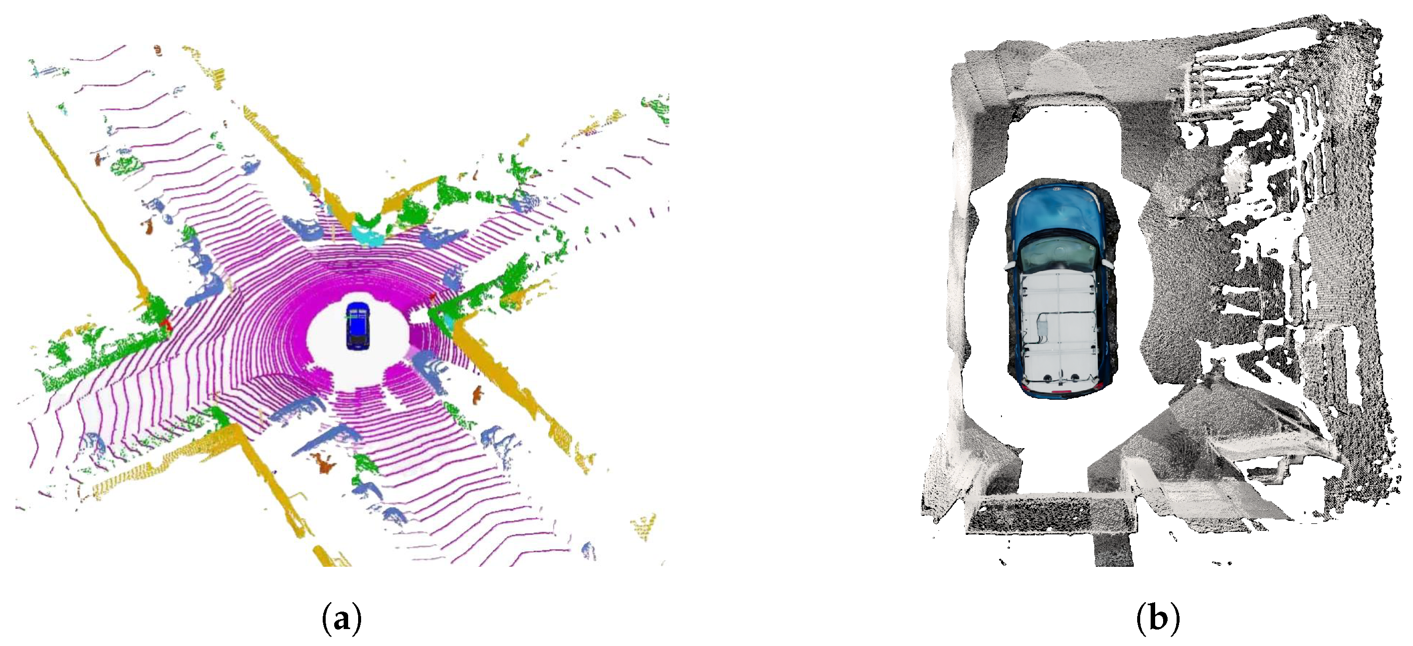
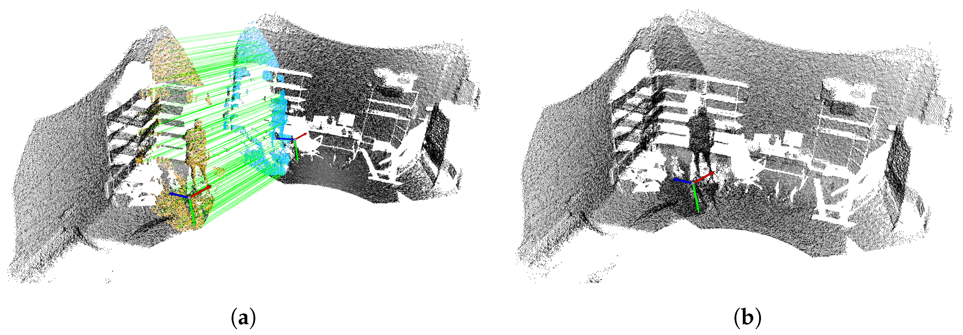
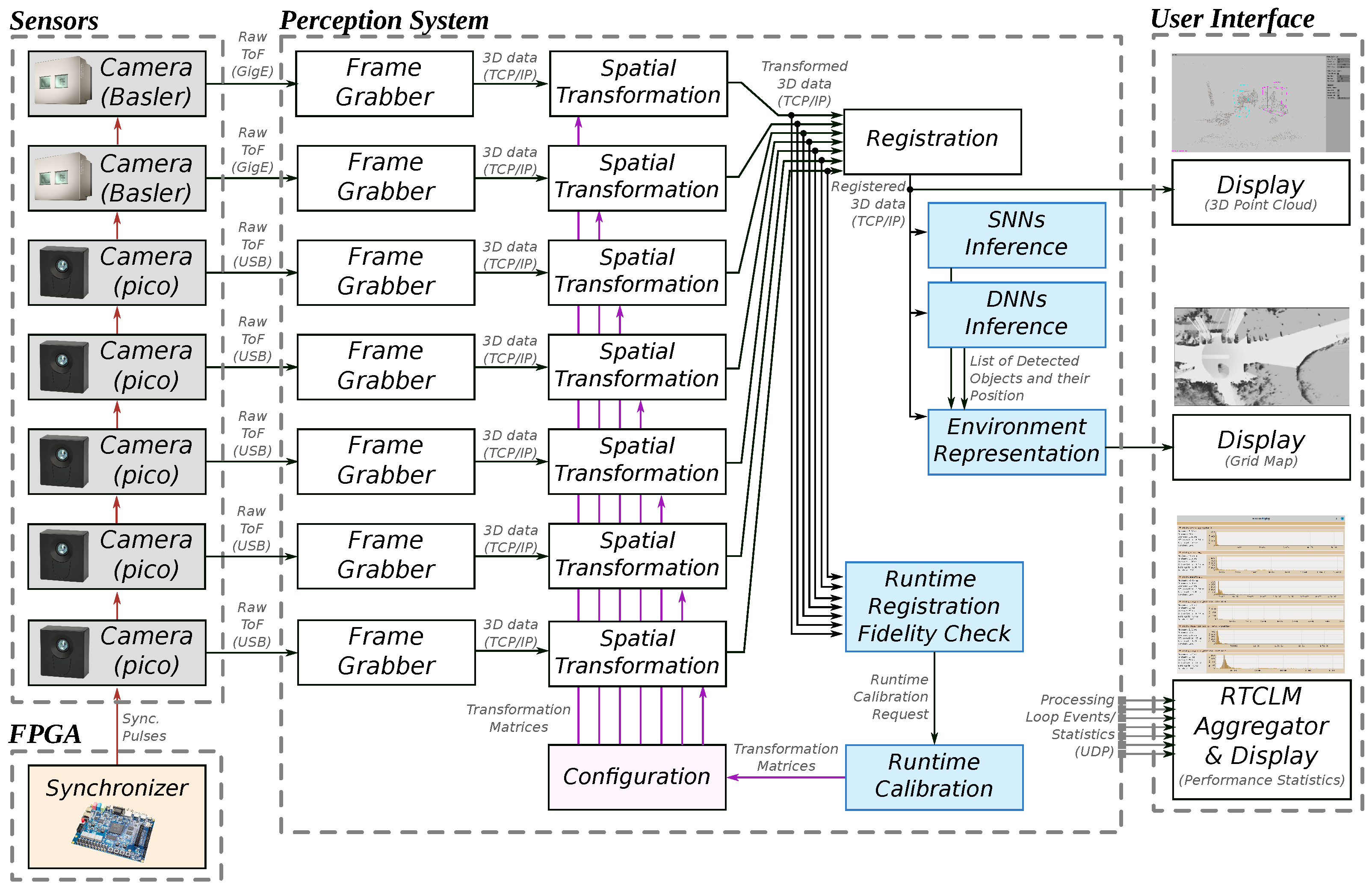
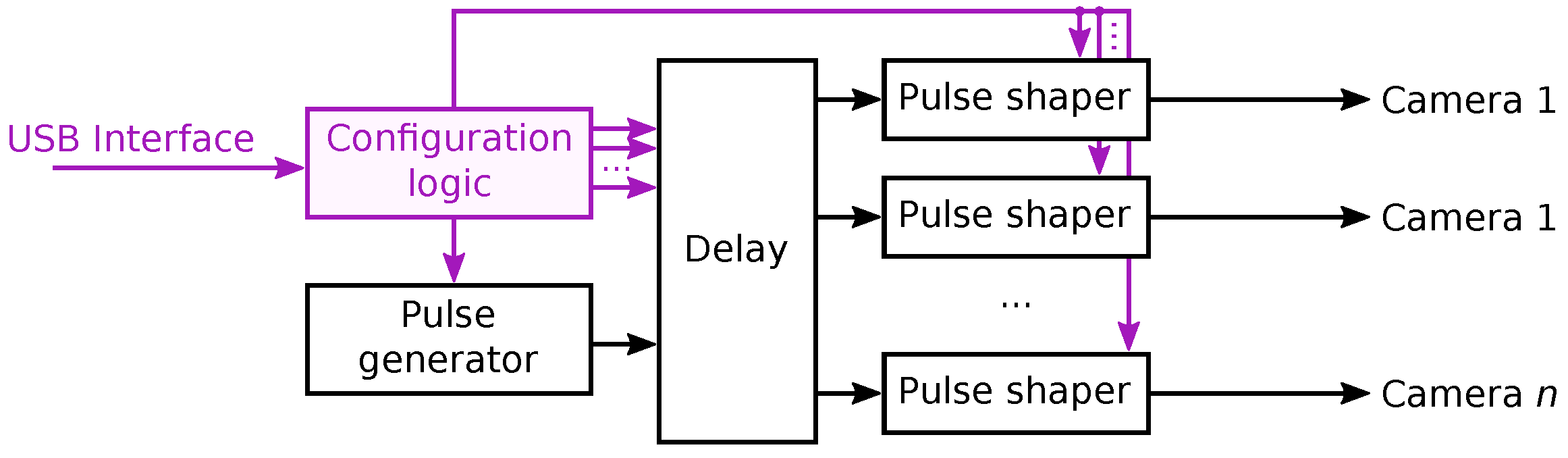
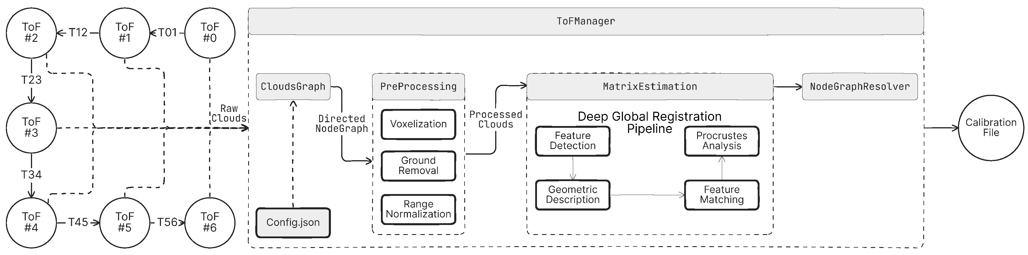
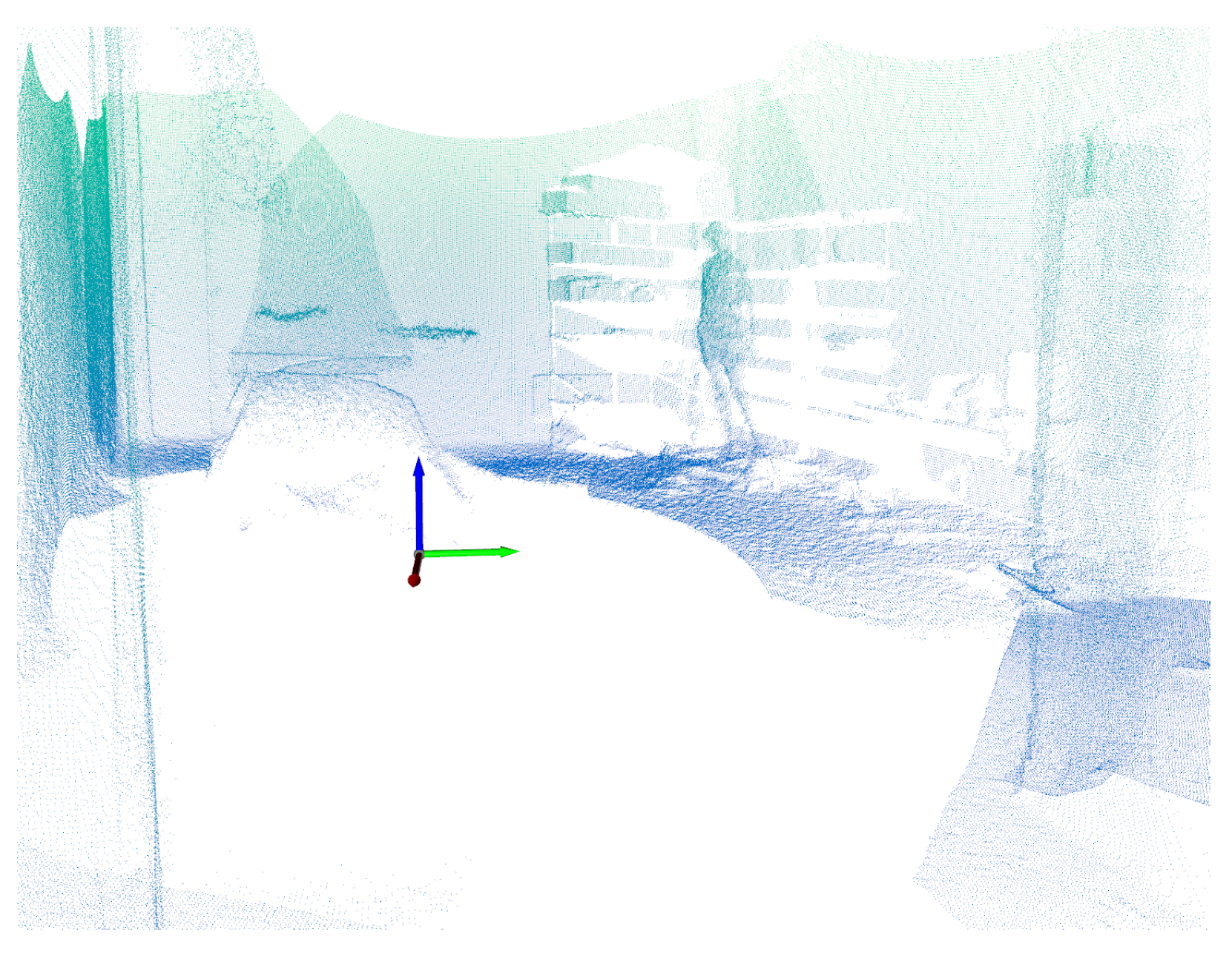
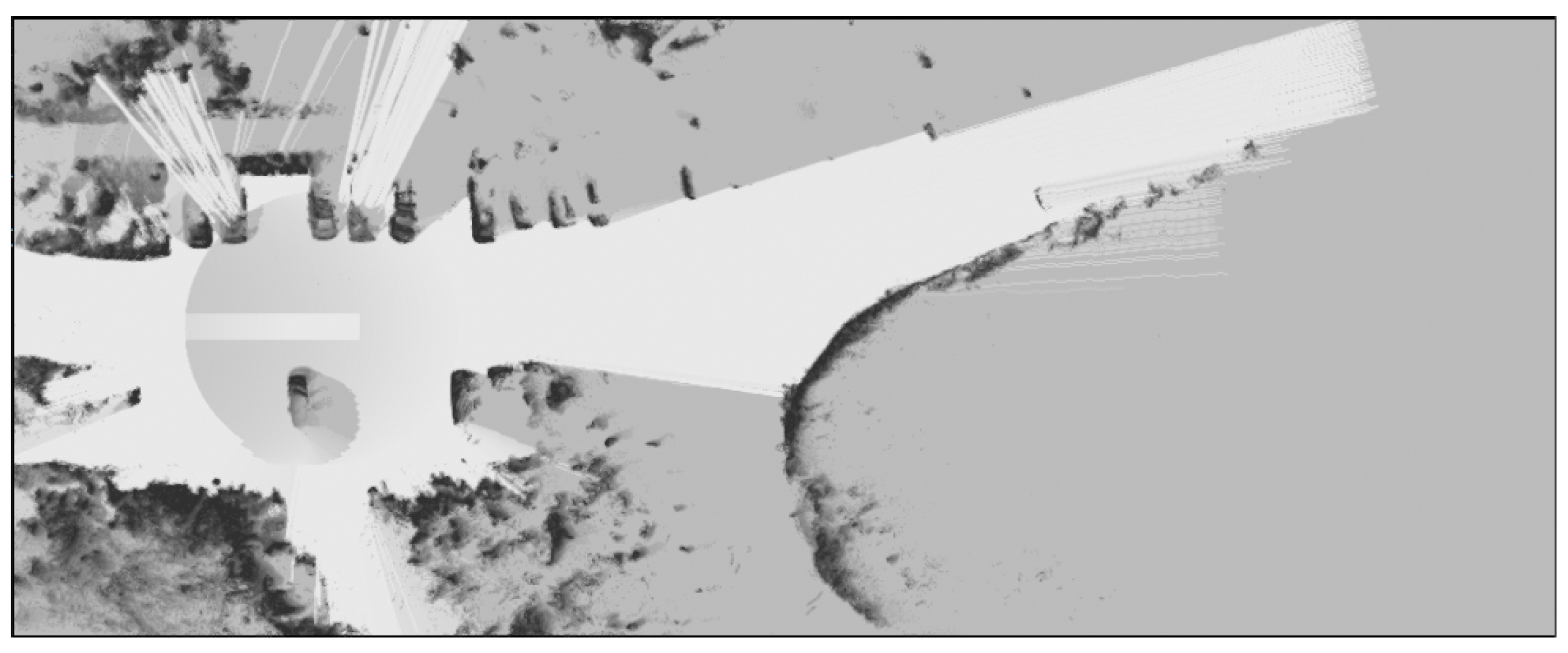
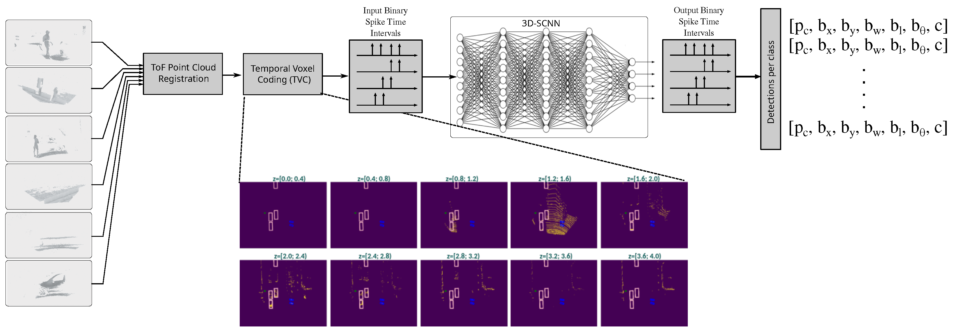
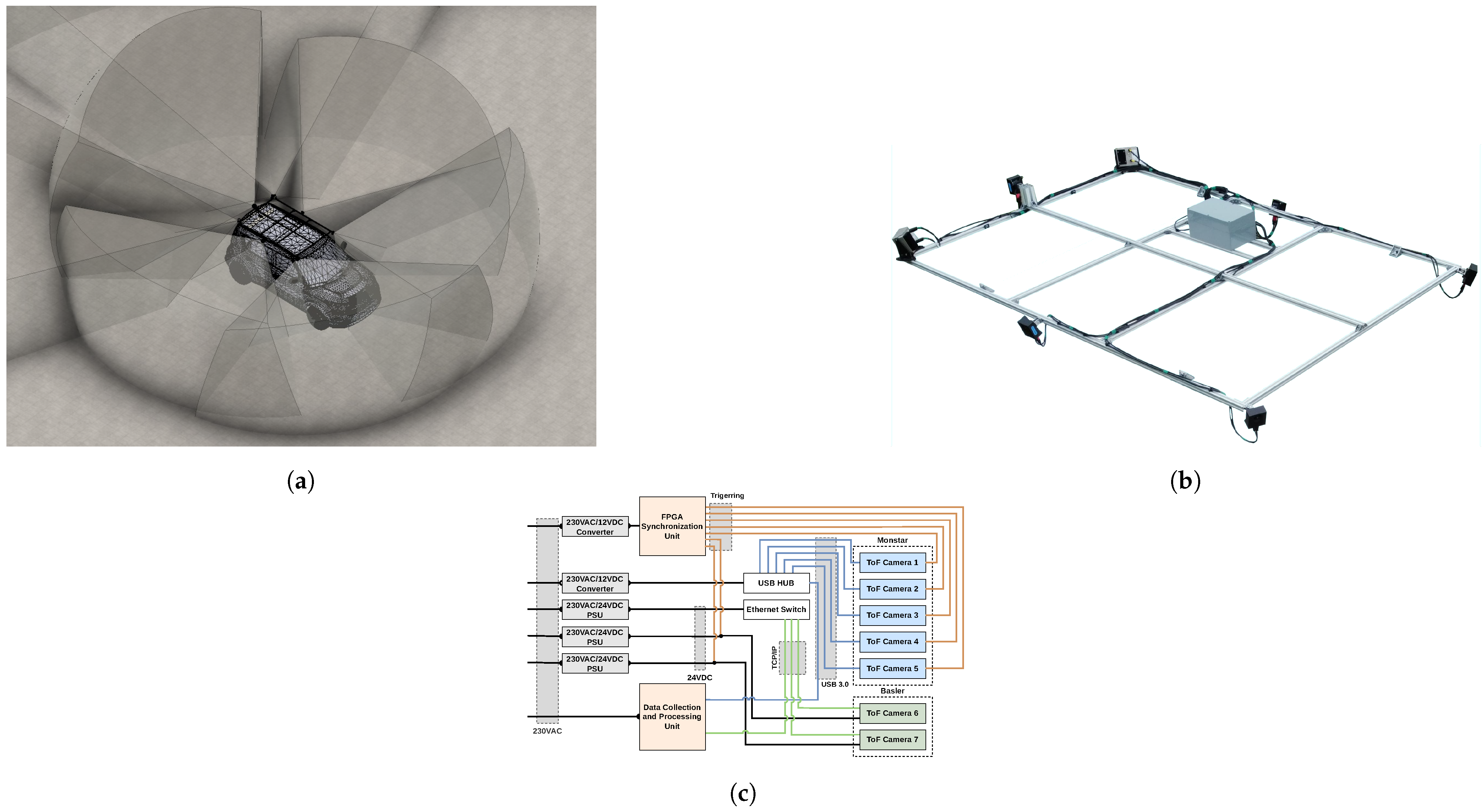
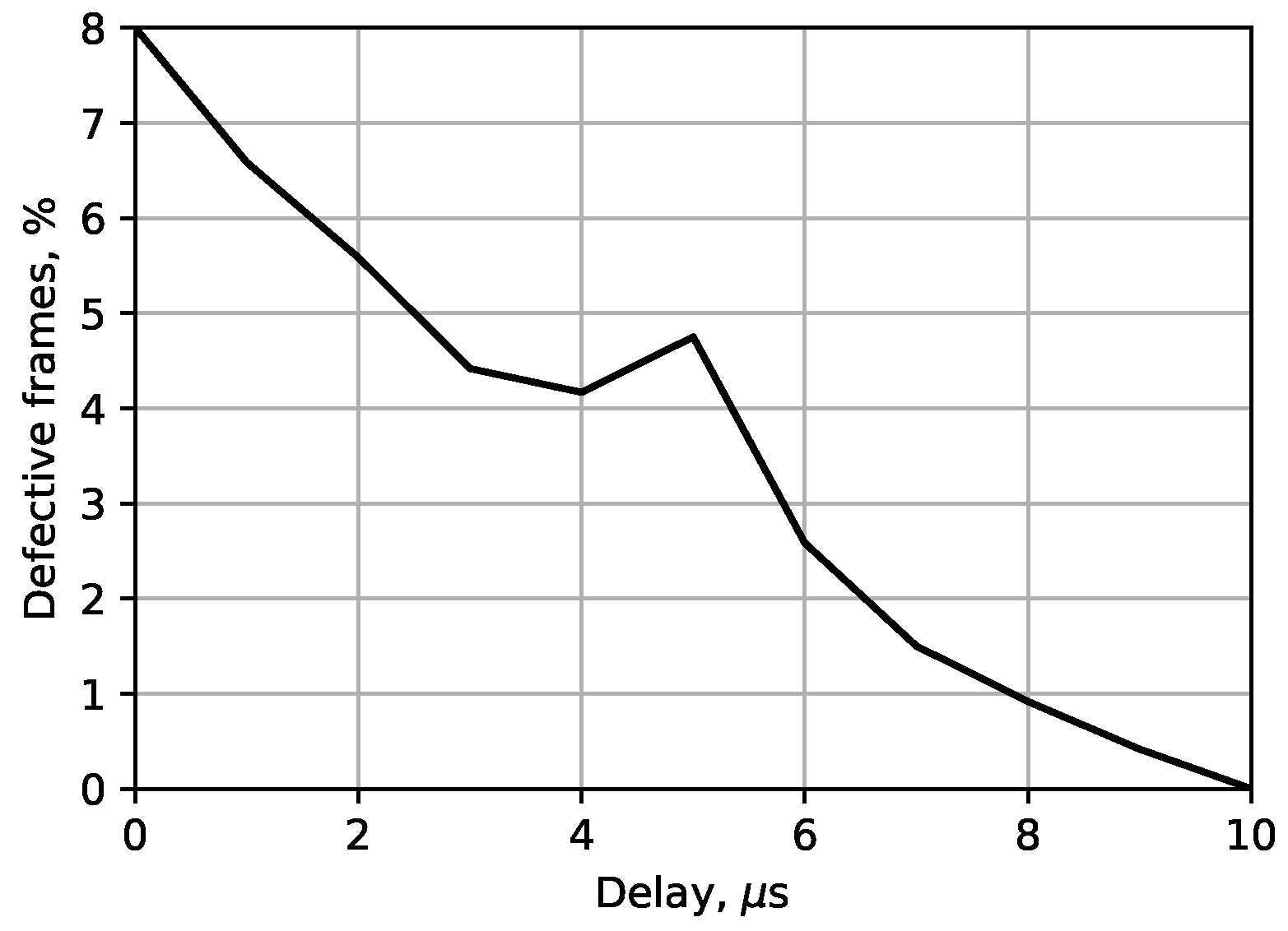
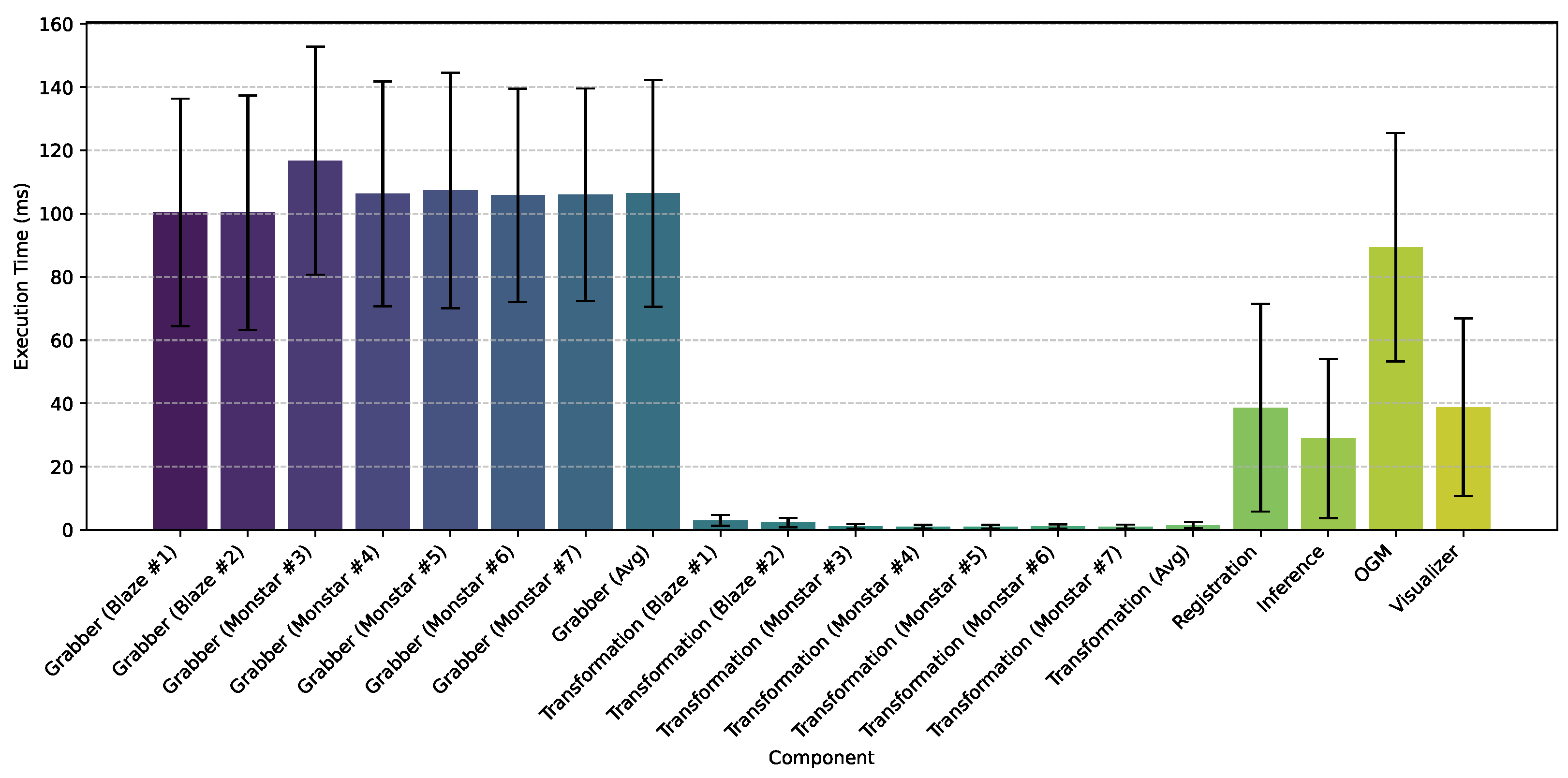
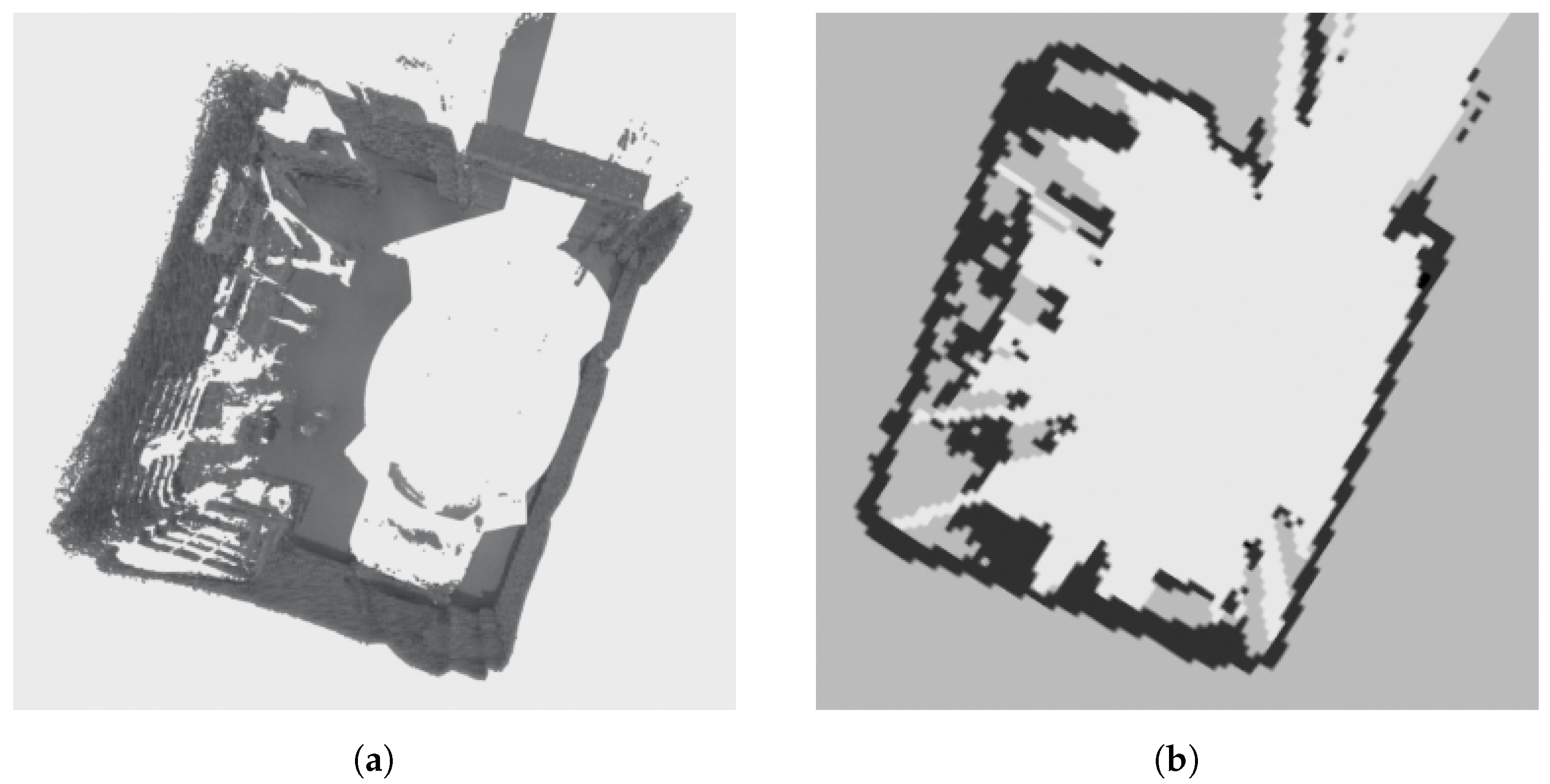
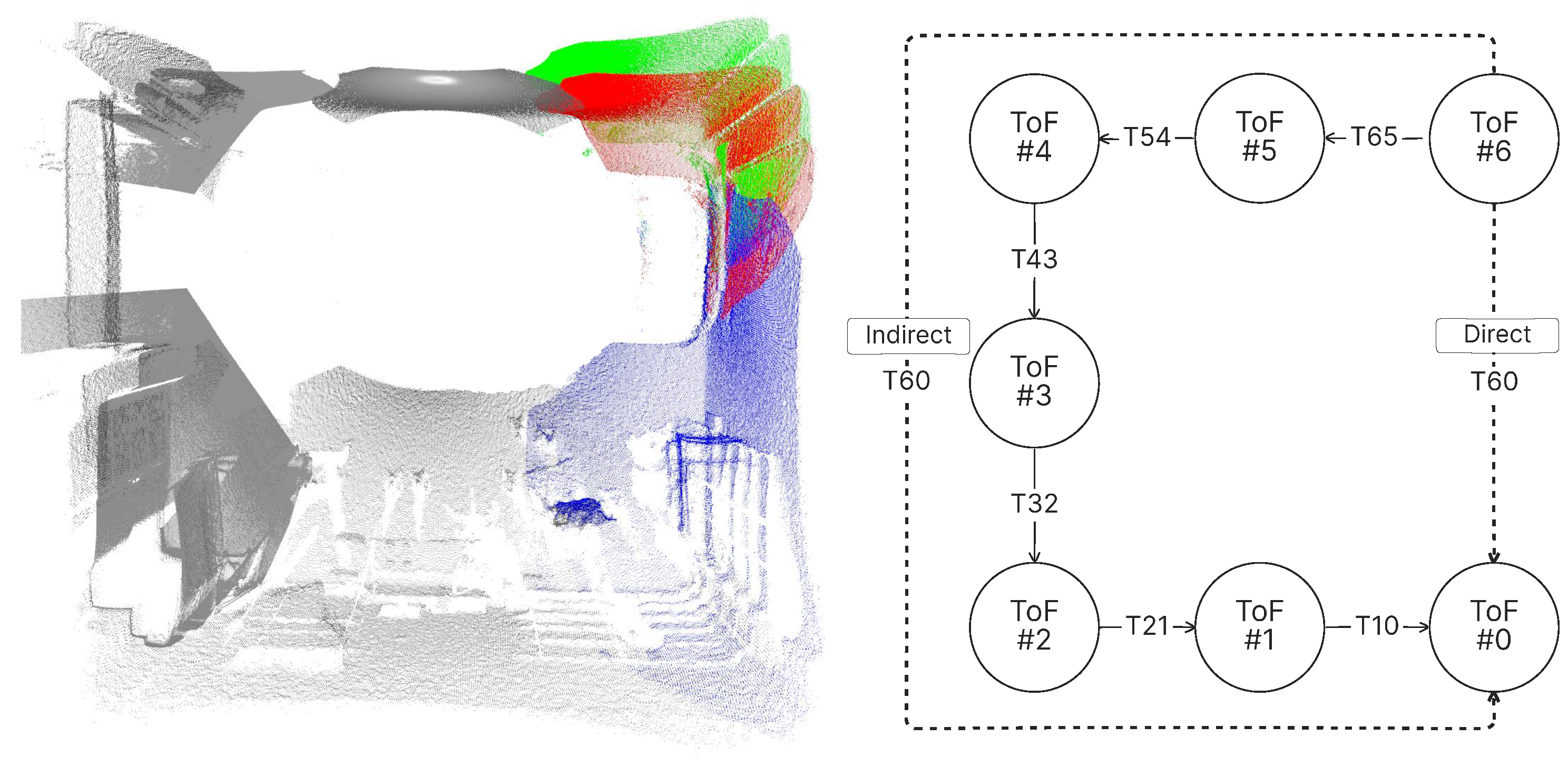
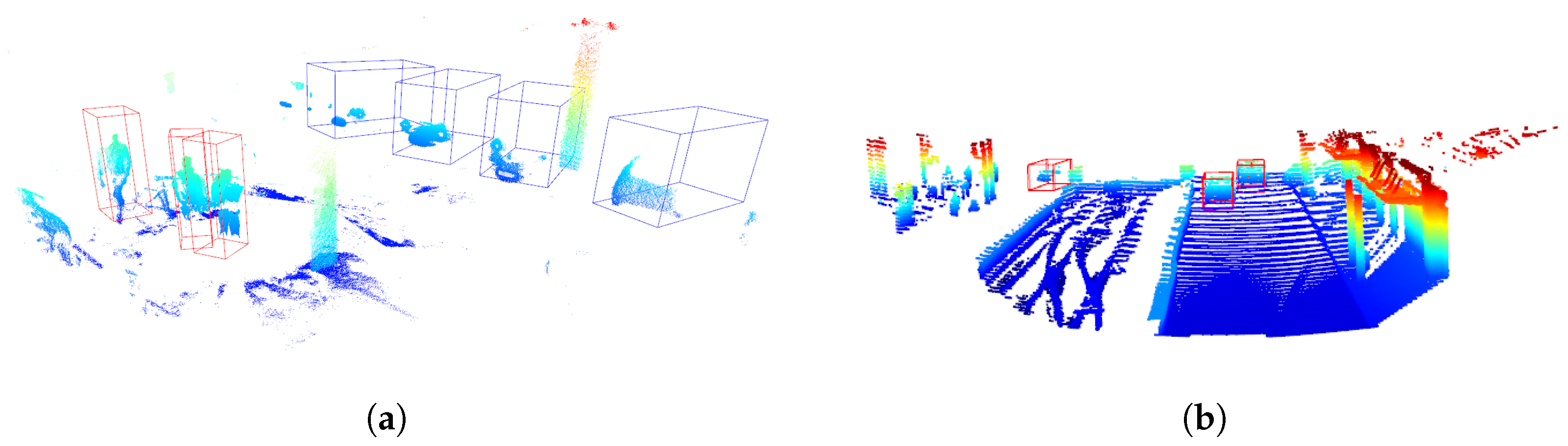
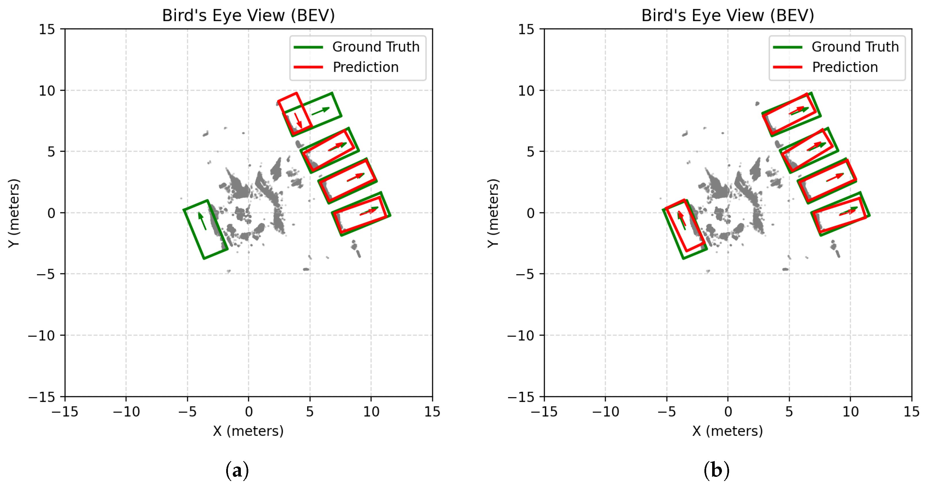

