Automatic Image Distillation with Wavelet Transform and Modified Principal Component Analysis

Abstract

Data distillation is an emerging research area, attracting the attention of machine learning (ML) and big data scientists and experts. The main goal of a distillation approach is to generate a compact dataset that preserves the essential characteristics of a larger one. In our study, we considered an initial large set of images and developed a novel method for distilling images from the initial set. The method combined discrete wavelet transform (DWT) and modified principal component analysis (M-PCA). Hence, our method first transforms images into vectors of low-band (LL) wavelet coefficients and then applies M-PCA to modify and reduce the number of vectors rather than their dimensionality. This distinguishes our approach from the traditional PCA method. We implemented the new method in Python 3.10 and validated it on public image databases, including Extended YaleB, digit-MNIST, and the ISIC2020. We demonstrated that creating a dictionary from a small set of distilled images and training a sparse representation wavelet-based classifier (SRWC) provides higher accuracy if compared to a classification when the SRWC method is trained with the entire initial training set of images.

1. Introduction

An important meta parameter in machine learning (ML) is the training set. For deep ML classifiers, extensive training datasets are required to achieve robust statistical results. If the large training sets also contain relatively high-resolution images, then the training process becomes extremely time-consuming. The training time could be significantly decreased if a smaller training dataset hosting the same features, qualities, statistical properties, and training abilities, is used.

Therefore, methods capable of generating or extracting, from a given large training set, a smaller one with the above abilities has become a subject of strong interest to the ML society. Early works in this field emerged around the middle of the last decade [1,2], with significant developments following in the subsequent years.

Methods for reducing training data while preserving data quality and model performance can be broadly categorized into two approaches: methods based on ML models [3,4,5] and data pruning (erasing) methods [6,7,8].

There is another concept gaining popularity among ML society, namely, transfer learning. It aims to develop methods and approaches that transfer knowledge across different tasks, for example, between image segmentation NN models and classification models [4]. Since knowledge transfer methods do not necessarily decrease the training time of the receiving model, we do not include them into the nomenclature of time reducing methods.

ML models for distillation use as a subject of their application knowledge and/or data. Knowledge distillation methods transfer meta parameters from teacher to student neural networks (NNs) [9,10,11]. Teacher NNs are generally large and complex, while student NNs are smaller and simpler as architecture. These teacher–student NN models significantly reduce the training time of student NNs, preserving the original training data and the statistical outcomes. They can solve problems in the fields of objects classification, detection, and segmentation in a variety of application areas in medicine and industry.

Data distillation methods keep the complexity and the architecture of the NN model the same but generate (distil) new data from the existing data. The distilled data has a smaller cardinality than the cardinality of the original training data, preserving its information quality and outcome statistics [5,12]. Note that in some cases, the newly distilled (generated) small-sized training set may contain images that do not visually resemble the original images at all [13]. Despite this dramatic change in the visual image features and the image theme, the distilled small image sets train the NN such that it provides the same or sometimes even better statistical measures. However, the visual form and the training ability of the ML distilled images depend on the number of epochs used in the process of distillation [14]. Note that this number could be high for some databases and may require more computer resources and longer run times, especially if the original images in the dataset are relatively sizable [14].

A comprehensive survey on the recent methods of data distillation, including the application of NNs, is given in [4]. The authors provide a detailed description of multiple data distillation techniques based on the concepts of “meta-model”, “gradient”, “distribution”, “trajectory”, and “factorization” matching.

On the other hand, data pruning methods are designed to remove less important and/or ill-defined samples from the original training set [6,7,15]. For the process of removal, pruning methods use optimization techniques to determine a sample’s importance [7]. Hence, optimization-based pruning methods can determine the smallest efficient training set from the original samples.

In 2024, ref. [8] published a new method capable of distilling vectors. This method was based on a modification of the principal components analysis (PCA) approach [16,17] and proved itself efficient for distilling vectors with relatively small dimensions. It improved the classification statistics of ML methods trained by sets augmented with distilled vectors. A disadvantage of the modified PCA distillation method is that training an ML classifier only with distilled vectors provides poor statistical outcomes.

In the present study, we developed a new method of image distillation that modifies training images and reduces the cardinality of the training set yet improves the classification accuracy of the ML classifier trained with this set. The new method does not apply ML techniques but was developed to reduce the training sample sets required in ML methods using, for example, sparse representation classification (SRC) [18,19]. These kinds of classifiers use a dictionary in the process of classification and the dictionary is designed by a set of atomic samples selected from the set of training samples.

The first part of the new distillation method consists of discrete wavelet transform (DWT) [20,21], which represents the image with the help of its low band (LL) wavelet coefficients. Further, we describe every image as a vector of LL wavelet coefficients and apply an adapted version of the modified PCA method [8] to generate a modified version of the vectors created by the image wavelet LL coefficients. Out of the modified vectors, we select the top m vectors from every modified class (matrix) and name them distilled vectors. They are used to build the distilled training dictionary of an SRC method. A block diagram that describes the new data distillation method is shown in Figure 1.

Note that m is a user-selected integer that should be smaller than the cardinality of the smallest class in the training image dataset. Even though we verified the new image distillation method by creating a distilled wavelet dictionary (DWD) for the sparse representation wavelet classification (SRWC) [19] method, the distilled images could be used for training in other ML methods including NNs.

The main contribution of the present study is the development of the DWD with the help of the new image distillation method, which implements the DWT, low-band wavelet (LL) coefficients (features), and a modified PCA method (M-PCA). The advantage one may obtain, if using our DWT-LL-M-PCA method, is a reduced set of training images that possess the same training capabilities as the entire original training set.

Further, this paper is organized as follows: Section 2 presents the DWT, shows an example of image wavelet decomposition, and describes the development of the training dictionary for the wavelet vectors of images; Section 3 describes the development of the new approach to modify the wavelet matrix of each training class with the help of the M-PCA method and the creation of the DWD; Section 4 comprises five subsections that describe the SRWC method, the public image databases YaleB [22] and MNIST (digit and fashion) [23,24], and ISIC2020 [25] used for the experiments, the metrics implemented to measure the effectiveness of the methods, the experimental scheme, and the results of image classification. This paper end with Section 5 and Section 6, which present the discussion and conclusions, where we comment on the comparisons between classifications with original and distilled training sets, list the contributions of the present study and its advantages, and outline the future work.

2. Wavelet-Based Training Dictionary Design

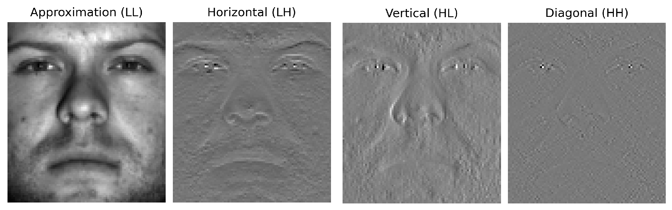
2.1. Image Decomposition to Wavelet Sub-Bands

In the context of two-dimensional signals, let I represent an image wherein $I\left(u,v\right)$ indicates the grey-level value at the pixel $(u,v)$. Implementing a single-level two-dimensional wavelet transformation for an image can be achieved utilizing the technique that employs the Haar kernels, introduced in [26]. Therefore, the half-band high-pass $G_H\left(k\right)$ and the half-band low-pass $G_L\left(k\right)$ filters can be characterized, in the spatial domain, by the Haar wavelet kerne, as shown below [26]:

$$G_H\left(k\right)=\left\{\begin{array}{cc}1,& 0⩽k<\raisebox{1ex}{$1$}\!\left/ \!\raisebox{-1ex}{$2$}\right.\\ -1,& \raisebox{1ex}{$1$}\!\left/ \!\raisebox{-1ex}{$2$}\right.⩽k<1\\ 0,& otherwise\end{array}\right.;G_L\left(k\right)=\left\{\begin{array}{cc}1,& 0⩽k<1\\ 0,& otherwise\end{array}\right..$$

(1)

Note that the high-pass filters $G_H\left(k\right)$ attenuate the low-band image features while passing the high-band image features. On the other hand, the low-pass filters $G_L\left(k\right)$ attenuate the high-band features while passing the low-band features. In the wavelet domain, the low-band features describe image overall properties, and structures as well as large-scale patterns. The high-band wavelet features describe details, like, corners, edges, and noise.

Further, 2D discrete wavelet transform (DWT) [20] decomposes an image into four distinct sub-bands: approximation (LL), vertical (HL), horizontal (LH), and diagonal (HH) components. Out of the four sub-bands, the following three are considered high-band features: LH, HL, and HH, while LL is considered as describing low-band features. An example of image decomposition to the four sub-bands is shown in Figure 2.

2.2. Training Wavelet Dictionary Design

Consider a set of total $N_k$ training images distributed in k different classes. Denote the i-th class of the training images with ${\xi }_i$ and the label of this class with $l_i$, for $i=1,\dots ,k$. The images in class ${\xi }_i$ we indicate with $I_{ij}$, where $I_{ij}\in R^{h_{ij}\times w_{ij}}$ and $h_{ij}$ denote the number of rows (height) in the image, while $w_{ij}$ denotes the number of columns (width) for $j=1,\dots ,n_i$, where $n_i$ denotes the number of images in class ${\xi }_i$. In connection with our further study, we resize the entire set of training images such that $I_{ij}\in R^{h\times w}$ for $i=1,\dots ,k$ and $j=1,\dots ,n_i$.

In the next step, using the 2D DWT, we decompose every image $I_{ij}\in {\xi }_i$ for $i=1,\dots ,k$ to the four wavelet coefficients LL, HL, LH, and HH. Following the idea introduced in [19], we flatten every image to a vector, where, for every image pixel, there is an LL wavelet value. Hence, we map every image $I_{ij}\in R^{h\times w}$ to a vector of the wavelet coefficient ${\mathbf{v}}_{\mathbf{ij}}\in R^{wh}$, which is a vector with $wh$ entries and the label $l_i$. Therefore, the class ${\xi }_i$ can be presented as the matrix ${\xi }_i={({\mathbf{v}}_{\mathbf{i}\mathbf{1}}\dots {\mathbf{v}}_{\mathbf{i}{\mathbf{n}}_{\mathbf{i}}})}^T\in R^{n_i\times hw}$, with its extended form being (${\xi }_i|{\mathbf{L}}_{\mathbf{i}}$), where ${\mathbf{L}}_{\mathbf{i}}={(l_i,l_i,\dots ,l_i)}^T\in R^{n_i}$, and $l_i\in R$ for $i=1,\dots ,k$.

If we vertically concatenate all training wavelet matrices ${\xi }_i$ we receive the matrix ${\mathbf{D}}_{\mathbf{t}}={({\xi }_1\dots {\xi }_k)}^T\in R^{N_k\times hw}$. Note that $N_k=n_1+n_2+\dots +n_k$, where $n_i$ for $i=1,\dots ,k$ is the cardinality of the i-th training class. We call matrix ${\mathbf{D}}_{\mathbf{t}}$ the training wavelet dictionary (TWD); its label’s extended form is $\left({\mathbf{D}}_{\mathbf{t}}\right|\mathbf{L})$, where the vector of labels $\mathbf{L}={({\mathbf{L}}_{\mathbf{1}},\dots ,{\mathbf{L}}_{\mathbf{k}})}^T\in R^{N_k}$.

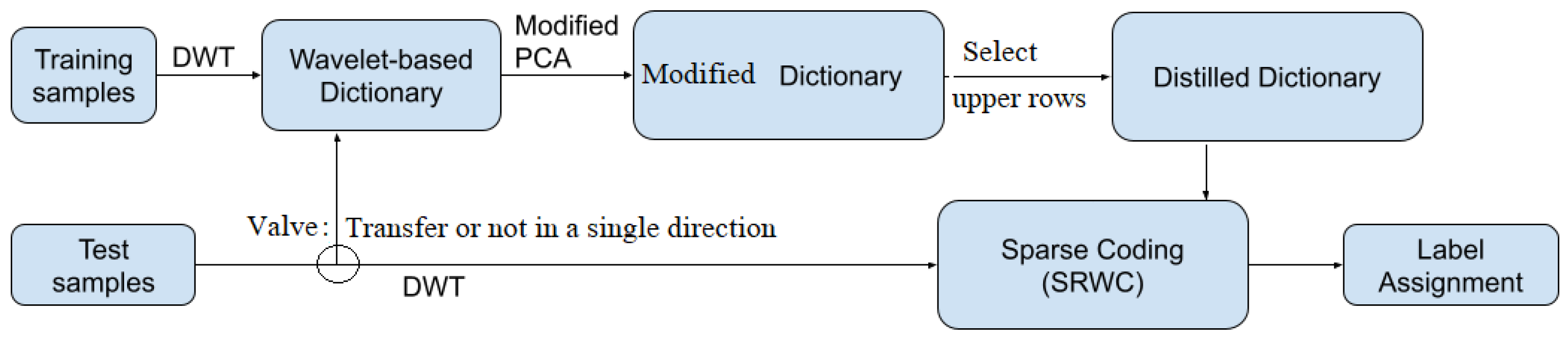
3. Distilling a Dictionary from the TWD

3.1. Modifying the Wavelet-Based Class Matrices

Consider TWD ${\mathbf{D}}_{\mathbf{t}}={({\xi }_1\dots {\xi }_k)}^T\in R^{N_k\times hw}$, constructed by the vectors of wavelet coefficients ${\mathbf{v}}_{\mathbf{ij}}\in R^{wh}$, $i=1,\dots ,k$ and $j=1,\dots ,n_i$. Denote ${\mathbf{v}}_{\mathbf{ij}}=(a_{ij}^1,\dots ,a_{ij}^{hw})$, where $a_{ij}^p\in R$ represents a wavelet coefficient, which we call a feature.

Analogously to [8], we construct the p-th feature vector of the i-th class with ${\mathbf{f}}_{\mathbf{i}}^{\mathbf{p}}=(a_{i1}^p,\dots ,a_{i{n}_i}^p)$, such that ${\mathbf{f}}_{\mathbf{i}}^{\mathbf{p}}\in {\mathbf{R}}^{{\mathbf{n}}_{\mathbf{i}}}$ and $p=1,\dots ,hw$. We then denote the mean of the feature vectors ${\mathbf{f}}_{\mathbf{i}}^{\mathbf{p}}$ with ${\mu }_i^p$ and the rank of the matrix ${\xi }_i$ with $r_i\le min\{n_i,hw\}$. Then, we normalize every wavelet coefficient LL as follows:

$$a_{iu}^p=a_{iu}^p-{\mu }_i^p,fori=1,\dots ,k,u=1,\dots ,n_i,andp=1,\dots ,hw.$$

(2)

Further, we calculate the covariance matrix, which measures the linear relationship between the features in the matrix (class) ${\xi }_i$ [17] for $i=1,\dots ,k$. For this purpose, we use the equation below and calculate every entry of the covariance matrix of the $i-th$ class, which we denote by ${\mathbf{F}}^{\mathbf{i}}=\left\{F_{qj}^i\right\},q=1,\dots ,hw,j=1,\dots ,hw$ [8]:

$$F_{qj}^i={\displaystyle \frac{1}{n_i-1}}\sum _{p=1}^{n_i}(a_{ij}^p-{\mu }_i^p)(a_{iq}^p-{\mu }_i^p).$$

(3)

In the next stage, we determine the Eigen vectors ${\mathbf{u}}_{\mathbf{j}}^{\mathbf{i}}\in R^{hw}$ and the Eigen values ${\lambda }_j^i$ of ${\mathbf{F}}^{\mathbf{i}}$ using the equation below, where $\mathbf{I}\in R^{hw\times hw}$ is the unit matrix:

$${\mathbf{F}}^{\mathbf{i}}{\mathbf{u}}_{\mathbf{j}}^{\mathbf{i}}={\lambda }_j^i{\mathbf{u}}_{\mathbf{j}}^{\mathbf{i}},|{\mathbf{F}}^{\mathbf{i}}-\lambda \mathbf{I}|=0,({\mathbf{F}}^{\mathbf{i}}-\lambda \mathbf{I}){\mathbf{u}}_{\mathbf{j}}^{\mathbf{i}}=\mathbf{0}.$$

(4)

Let us consider the pairs $({\lambda }_j^i,{\mathbf{u}}_{\mathbf{j}}^{\mathbf{i}})$, where $j=1,\dots ,hw$. Recall that $hw$ is the number of features in ${\xi }_i$, while $r_i\le min\{n_i,hw\}$ is its rank. Recall that the number of classes in ${\mathbf{D}}_{\mathbf{t}}$ is k. We now select the integer $m\le r_i$ and find the m largest Eigen values ${\lambda }_{j_1}^i\ge \dots \ge {\lambda }_{j_m}^i$ as well as their corresponding Eigen vectors ${\mathbf{u}}_{{\mathbf{j}}_{\mathbf{1}}}^{\mathbf{i}},\dots ,{\mathbf{u}}_{{\mathbf{j}}_{\mathbf{m}}}^{\mathbf{i}}$. Then, we construct the matrix ${\mathbf{T}}^{\mathbf{i}}\in {\mathbf{R}}^{\mathbf{hw}\times \mathbf{m}}$ according to decreasing Eigen values from right to left:

$${\mathbf{T}}^{\mathbf{i}}=[{\mathbf{u}}_{{\mathbf{j}}_{\mathbf{1}}}^{\mathbf{i}},{\mathbf{u}}_{{\mathbf{j}}_{\mathbf{2}}}^{\mathbf{i}},\dots ,{\mathbf{u}}_{{\mathbf{j}}_{\mathbf{m}}}^{\mathbf{i}}],$$

(5)

where every Eigen vector ${\mathbf{u}}_{{\mathbf{j}}_{\mathbf{l}}}^{\mathbf{i}}\in R^{hw}$ and m are the user-selected integer. The idea behind the construction of matrix ${\mathbf{T}}^{\mathbf{i}}$ is the concept that the larger the Eigen value, the stronger the influence of its Eigen vector.

Recall that the class matrix ${\xi }_i\in R^{n_i\times hw}$. Therefore, the matrix product below,

$${\xi }_i{\mathbf{T}}^{\mathbf{i}}={\mathcal{D}}^{\mathbf{i}},$$

(6)

maps the matrix of the $i-th$ class to a transformed one ${\mathcal{D}}^{\mathbf{i}}\in R^{n_i\times m}$ for $i=1,\dots ,k$. The next left product with the matrix ${\left({\mathbf{T}}^{\mathbf{i}}\right)}^{\mathbf{T}}\in {\mathbf{R}}^{\mathbf{m}\times \mathbf{hw}}$ maps the transformed matrix ${\mathcal{D}}^{\mathbf{i}}$,

$${\mathcal{D}}^{\mathbf{i}}{\left({\mathbf{T}}^{\mathbf{i}}\right)}^{\mathbf{T}}={\mathbf{\Delta }}^{\mathbf{i}},$$

(7)

into the original space such that ${\mathbf{\Delta }}^{\mathbf{i}}\in {\mathbf{R}}^{{\mathbf{n}}_{\mathbf{i}}\times \mathbf{hw}}$. Note that unless ${\mathbf{T}}^{\mathbf{i}}{\left({\mathbf{T}}^{\mathbf{i}}\right)}^{\mathbf{T}}=\mathbf{I}$, where $\mathbf{I}\in R^{hw\times hw}$ is the unit matrix, the new matrix ${\mathbf{\Delta }}^{\mathbf{i}}\ne {\xi }_i$. Hence, we call the matrix ${\mathbf{\Delta }}^{\mathbf{i}}$ the modified matrix of the i-th training class.

Please note that the modified version of the PCA method described above decreases the number of vectors in a set, while the original PCA decreases the dimension of the vectors in the set.

3.2. Creating a Distilled Wavelet Dictionary

Recall that we vertically concatenated the original classes of wavelet vectors to receive the training wavelet dictionary (TWD) ${\mathbf{D}}_{\mathbf{t}}={({\xi }_1,\dots ,{\xi }_k)}^T={({\mathbf{v}}_{\mathbf{11}},\dots ,{\mathbf{v}}_{\mathbf{1}{\mathbf{n}}_{\mathbf{1}}},\dots ,{\mathbf{v}}_{\mathbf{k}\mathbf{1}},\dots ,{\mathbf{v}}_{\mathbf{k}{\mathbf{n}}_{\mathbf{k}}})}^T\in R^{N_k\times hw}$. If we do the same with the modified training matrices (classes) ${\mathbf{\Delta }}^{\mathbf{i}}$ for $i=1,\dots ,k$, we receive the modified training wavelet dictionary

$${\mathbf{\Delta }}_{\mathbf{t}}={({\mathbf{\Delta }}^{\mathbf{1}},\dots ,{\mathbf{\Delta }}^{\mathbf{k}})}^T={({\mathbf{v}}_{\mathbf{11}}^{\mathbf{d}},\dots ,{\mathbf{v}}_{\mathbf{1}{\mathbf{n}}_{\mathbf{1}}}^{\mathbf{d}},\dots ,{\mathbf{v}}_{\mathbf{k}\mathbf{1}}^{\mathbf{d}},\dots ,{\mathbf{v}}_{\mathbf{k}{\mathbf{n}}_{\mathbf{k}}}^{\mathbf{d}})}^T\in R^{N_k\times hw}.$$

(8)

Note that in the present notation of vectors, the superscript $\mathbf{d}$ denotes that the vectors are modified.

Recall also that the modified training wavelet matrices ${\mathbf{\Delta }}^{\mathbf{i}}$ are obtained by two left multiplications (see Equations (6) and (7)) of the original training wavelet matrices ${\xi }_i$ for $i=1,\dots ,k$. Since the multiplication of matrices does not change the order of the rows, it follows that the rows in ${\mathbf{\Delta }}_{\mathbf{t}}$ are modified versions of the rows in ${\mathbf{D}}_{\mathbf{t}}$.

To create the training distilled wavelet dictionary (DWD), we select the upper m vector rows from every modified matrix (class) of training wavelet vectors ${\mathbf{\Delta }}^{\mathbf{i}}$ for $i=1,\dots ,k$. Concatenating the k selected sets of m modified vectors, we receive the distilled wavelet dictionary (DWD):

$${\mathbf{\Delta }}_{\mathbf{t}}^{\mathbf{d}}={({\mathbf{\Delta }}_{\mathbf{d}}^{\mathbf{1}},\dots ,{\mathbf{\Delta }}_{\mathbf{d}}^{\mathbf{k}})}^T={({\mathbf{v}}_{\mathbf{11}}^{\mathbf{d}},\dots ,{\mathbf{v}}_{\mathbf{1}\mathbf{m}}^{\mathbf{d}},\dots ,{\mathbf{v}}_{\mathbf{k}\mathbf{1}}^{\mathbf{d}},\dots ,{\mathbf{v}}_{\mathbf{k}\mathbf{m}}^{\mathbf{d}})}^T\in R^{km\times hw}.$$

(9)

Note that ${\mathbf{\Delta }}_{\mathbf{d}}^{\mathbf{i}}$ contains only the selected m upper rows (vectors) from the matrix of the modified training wavelet class ${\mathbf{\Delta }}^{\mathbf{i}}$. Thus, the number of training vectors (rows) in the DWD ${\mathbf{\Delta }}_{\mathbf{t}}^{\mathbf{d}}$ is $mk<<N_k$ and the number of vectors in the modified training wavelet dictionary is ${\mathbf{\Delta }}^{\mathbf{i}}$. Also, the selected vectors ${\mathbf{v}}_{\mathbf{ij}}^{\mathbf{d}}\in R^{h\times w}$, which complies with $I_{ij}\in R^{h\times w}$.

4. Experimental Validation

In the present section, we first introduce the classifier sparse representation wavelet-based classification (SRWC), which we used to measure statistics when conducting training with original and distilled sets of the training dictionary. Recall that the set of distilled training images is smaller than the set of original images.

Next, we introduce the image databases and metrics that were used for the purpose of measurement. In the last subsection, we describe the experimental procedure and the results obtained by the SRWC method when using original TWD and DWD.

4.1. Sparse Representation Wavelet-Based Classification

The sparse representation wavelet-based classification (SRWC) method [19] was implemented in the wavelet domain to construct a feature dictionary derived from training samples. Paper [19] demonstrates that utilizing features exclusively from low-pass sub-band (LL) wavelet coefficients can significantly enhance image classification performance. Hence, we used the low-pass sub-band coefficients LL to generate the TWD.

The preprocessing techniques for the TWD design applied several steps, including the following: labeling the k training classes and conducting principal component analysis (PCA) to reduce the dimensionality of each vectorized sample, named “atom”. As shown in Section 2.2, for each class i, the vectorized training atoms ${\mathbf{v}}_{\mathbf{i}\mathbf{j}},j=1,\dots ,n_i$, creating a sub-dictionary matrix ${\xi }_i={({\mathbf{v}}_{\mathbf{i}\mathbf{1}},\dots ,{\mathbf{v}}_{\mathbf{i}{\mathbf{n}}_{\mathbf{i}}})}^T\in R^{n_i\times hw}$, where $hw$ represents the dimension of each vectorized training atom and $n_i$ denotes the number of atoms within the class. Aggregating $N_k$ atoms from k categories (classes), the comprehensive walet training matrix of original vectors was constructed as ${\mathbf{D}}_{\mathbf{t}}={({\xi }_1,\dots ,{\xi }_k)}^T$ and modified to ${\mathbf{\Delta }}_{\mathbf{t}}$ with Equation (7), where every modified class ${\mathbf{\Delta }}^{\mathbf{i}}={({\mathbf{v}}_{\mathbf{i}\mathbf{1}}^{\mathbf{d}},\dots ,{\mathbf{v}}_{\mathbf{i}{\mathbf{n}}_{\mathbf{i}}}^{\mathbf{d}})}^T\in R^{n_i\times hw}$ was distilled to ${\mathbf{\Delta }}_{\mathbf{d}}^{\mathbf{i}}={({\mathbf{v}}_{\mathbf{i}\mathbf{1}}^{\mathbf{d}},\dots ,{\mathbf{v}}_{\mathbf{i}\mathbf{m}}^{\mathbf{d}})}^T\in R^{m\times hw}$.

Based on the assumption of sparse representation, a new unknown test atom ${\mathbf{x}}^{\mathbf{T}}={({\mathbf{x}}_{\mathbf{i},\mathbf{1}},\dots ,{\mathbf{x}}_{\mathbf{i},\mathbf{hw}})}^T\in {\mathbb{R}}^{hw\times 1}$ was associated with a specific class i if represented as a sparse linear combination of atoms associated with this class:

$$\mathbf{y}={\mathbf{x}}_{i,1}{\mathbf{v}}_{i,1}^d+{\mathbf{x}}_{i,2}{\mathbf{v}}_{i,2}^d+\dots +{\mathbf{x}}_{i,m}{\mathbf{v}}_{i,m}^d,$$

(10)

where ${\mathbf{x}}_{i,j}\in \mathbb{R},j=1,2,\dots ,m$ constitutes the sparse vector coefficients corresponding to class i. The sparse classification methodology centered on identifying the most appropriate set of training atoms for best approximation of $\mathbf{y}$. This was accomplished by determining a sparse approximation vector $\widehat{\mathbf{x}}$ with non-zero entries associated with the $i^{th}$ class, resolved through the following Lasso optimization formulation [19]:

$$\widehat{\mathbf{x}}=\underset{\mathbf{x}}{\min }{∥\mathbf{y}-{\mathbf{\Delta }}_{\mathbf{t}}^{\mathbf{d}}\mathbf{x}∥}_2^2+{\lambda }_0{∥\mathbf{x}∥}_1.$$

(11)

The classification of the unknown vector $\mathbf{x}$ was ultimately determined by analyzing the non-zero coefficients within $\widehat{\mathbf{x}}$. The final classification was executed by minimizing the discrepancy between the sparse sample and the original representation:

$$clas{s}_{pred}\left(\mathbf{y}\right)=\arg \underset{i}{\min }{∥\mathbf{y}-{\mathbf{\Delta }}_{\mathbf{t}}^{\mathbf{d}}{\delta }_i\left(\widehat{\mathbf{x}}\right)∥}_2,$$

(12)

where $\widehat{\mathbf{x}}\in {\mathbb{R}}^m$, ${\delta }_i$ is a characteristic function that selects elements in $\widehat{\mathbf{x}}$ that are associated with class i.

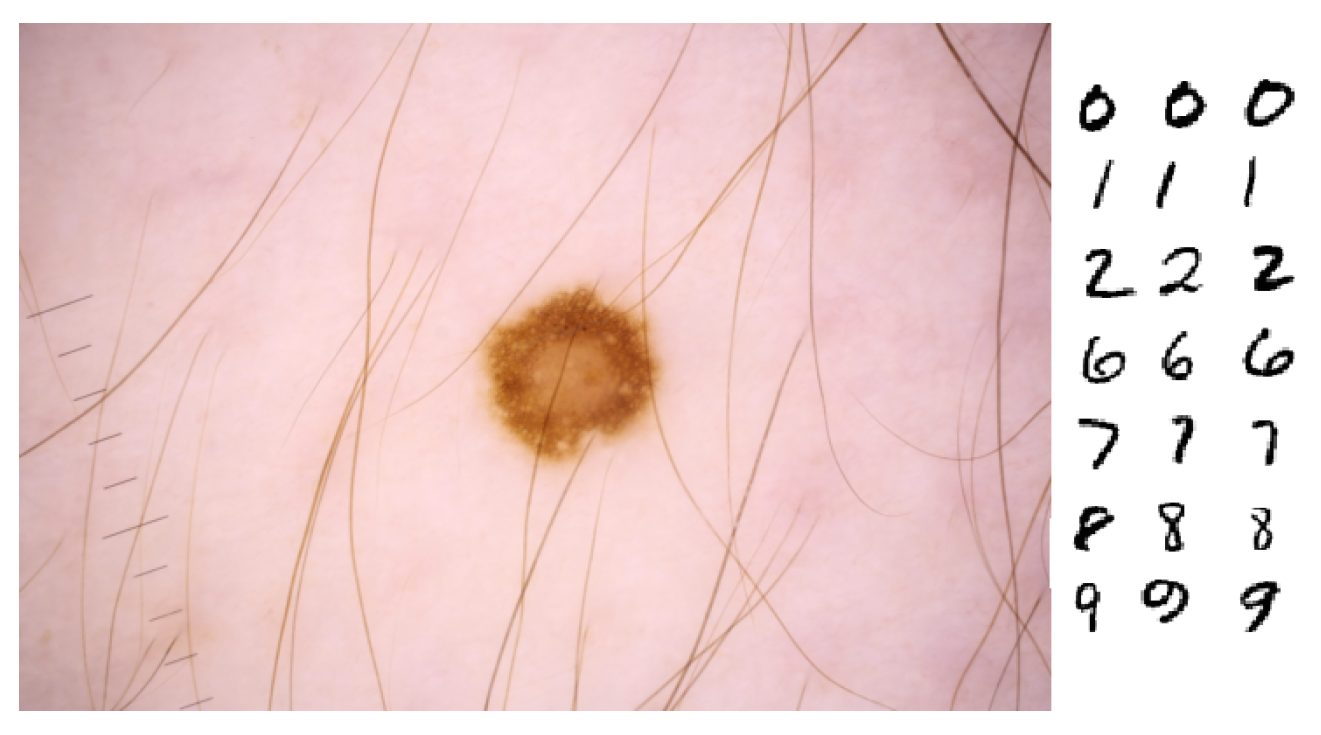
4.2. Original Datasets

To experimentally validate the new image distillation method based on the DWT, LL wavelet coefficients, and M-PCA methods, we used the public image databases YaleB [22], digit-MNIST [24], and ISIC2020 [25].

The YaleB [22] database contains 2414 frontal-face images of size $192\times 168$ taken from 38 faces. Therefore, the database consists of 38 classes and every class contains 64 pictures taken under different illumination conditions.

The public image database digit-MNIST [24] consists of 60,000 hand-written images of digits for training and 10,000 hand-written digit images for testing. Both the training and testing sets are split into 10 distinct classes. Every image has a size 28 × 28 pixels.

The most recent skin lesion image database is ISIC2020 [25]. It contains of 33,126 training images and 10,982 unlabeled benign and malignant images for testing. The training samples are split into 32,542 benign and 584 malignant. Experienced clinicians and dermatologists labeled the training images. The original image sizes vary between [480, 6000] for the number of rows and between [640, 6000] for the number of columns. To standardize the images, we resized them to $256\times 192$ and $332\times 590$ pixels. In Figure 3, we show an original training sample from ISIC2020, resized from $6000\times 4000$ to $590\times 332$ pixels. On the right side of the same figure, we show original training samples from digit-MNIST.

4.3. Classification Metrics

The notations TP = True Positives, TN = True Negatives, FP = False Positives, and FN = False Negatives usually describe the outcomes from a classification method. Also, they are implemented in the calculation of accuracy, the most often used metrics to evaluate the effectiveness of classification.

• Accuracy (AC): measures the overall correctness of a model’s predictions:

  $$\mathrm{AC}={\displaystyle \frac{\mathrm{TP}+\mathrm{TN}}{\mathrm{TP}+\mathrm{TN}+\mathrm{FP}+\mathrm{FN}}}.$$

4.4. Experimental Schemes

Our experimental scheme consisted of two major stages. In the first one, we distilled m number of images applying the DWT [20], LL, and M-PCA [8] methods. In the next stage, we trained the SRWC method with original images and classified original testing images. Afterward we train the same classifier under the same conditions and parameters but with distilled samples and classify distilled training images (Case 1) or original training images (Case 2 and Case 3, defined below).

If the training or testing was conducted with the entire original or distilled training/testing image dataset, a single classification was performed. But, if a smaller number of training or testing original or distilled images was used, we implemented the Monte Carlo scheme [27] to select the necessary set for conducting the experiments. This scheme increased the statistical objectivity of the classification results and consisted of n runs of the classifier under the same conditions and parameters but with different sets of training samples. At the end, the average of the experimental outcomes was calculated and used for comparisons. In most cases, $n=5$ or $n=10$ was named 5-fold or 10-fold cross-validation, respectively.

4.5. Experimental Results

To validate our new method for training image dataset distillation, based on the DWT [20], LL wavelet coefficients, and M-PCA [8], we implemented it in Python alongside the SRWC method [19]. Employing the code, we conducted three kinds of experiments with the public image databases described in Section 4.2.

In the first kind of experiment, namely, Case 1, we distilled images from the union of the training and testing vectors (recall that every image was presented as a vector of LL wavelet coefficients) of every class. Then, we split the distilled vectors (images) into training and testing sets for every class. Further, we created the DWD by concatenating the distilled training vectors from all classes. Similarly, we merged the distilled testing vectors from all classes to form the test set for each experiment. The experimental results, which provide four different number of distilled vectors (images) from the image database YaleB, are presented in

Table 1. Accuracy (Ac) results obtained by the SRWC method [19] applied to the original YaleB image database and classifications results with distilled images from each of the 38 classes of YaleB implementing Case 1 and Case 2. In the Ac column the highest value is in bold.

	Training per Class	Total for 38 Classes	Train/Test per Class	Ac%
Original images YaleB-38 classes	64	2432	30/34	98.06% [28]
Case 1 setup for YaleB-38 classes
Distilled images 1st experiment	57	2166	30/27	98.9%
Distilled images 2nd experiment	44	1672	30/14	98.72%
Distilled images 3rd experiment	38	1444	30/8	$\mathbf{99}.\mathbf{29}\%$
Distilled images 3rd experiment	32	1216	30/2	98.7%
Case 2 setup for YaleB-38 classes
Distilled images	18	684	18/26	91.5%

. An image from this database and a sample from its DWD ${\Delta }_t^d$ are shown in Figure 4.

In the second kind of experiment, named Case 2, we distilled training vectors (images) from the original training and testing sets of every class. Further, we used the distilled vectors to construct the DWD, which we applied to train the SRWC [19] method and classify a randomly selected subset of original testing vectors (images). The selection was conducted with the Monte Carlo scheme [27]. The experimental results obtained with distilled images when applying the present distillation Case 2 are presented at the bottom of Table 1, where we show the classification results when training with distilled images from Yale B.

In the distillation Case 3, we distilled training (images) only from the original training set of every class. Then, we created the DWD, trained the SRWC method, and classified the original testing vectors (images). The experimental results with the present setup and the image databases digit-MNIST and ISIC2020 are shown in

Table 2. Accuracy (Ac) results obtained by SRWC [19] for the images distilled from digit-MNIST implementing the distillation described in Case 3. In the Ac column the highest value is in bold.

	Training per Class	Total for 38 Classes	Train/Test per Class	Ac %
Original images digit-MNIST-10 classes	600	6000	600/1000	11%
Original images digit-MNIST-10 classes	1000	10,000	1000/1000	14.19%
Case 3 setup for digit-MNIST-10 classes
Distilled images 1st experiment	157	1570	157/1000	95.25%
Distilled images 2nd experiment	94	940	94/1000	$93.84\%$

and

Table 3. The 2nd and most left columns show results of classifying, by the SRWC method, the 10,982 original testing ISIC2020 images. The 3rd column shows results when the original training and testing images are sharpened by Laplace operator. All results are in "score" metric evaluated in the ISIC2020 web page [25]. The highest value is in bold.

Training Samples (Malignant/Benign)	Original Images	Sharpened with Laplacian	Distilled Under Case 3 Setup
292/584	score = 0.7734 [28]	score = 0.7804 [28]	score = 0.7336
523/7704	-	-	score = 0.8115

.

5. Discussion

Examining the results in Table 1 for the Case 1 distillation and classification, we observe that the accuracy (Ac) achieved with the four distilled sets was higher than the Ac obtained with the original dataset. Note that the number of distilled training images for all experiments was the same (30), while the set of distilled testing images decreased. The largest Ac = $99.29\%$ was achieved in the 3rd experiment, when we distilled 1444 images out of the 2432 original images.

These results suggest that distilling from the combined training and testing sets improved classification accuracy, even when the total number of images used was reduced. However, this approach was feasible only if the distilled training images could be identified, as demonstrated with the SRWC method.

Recall that in Case 2, we distilled both training and testing images. Then, we used the distilled images for training and tested a set of original images. The experiment in this case with the Yale B dataset is presented at the bottom of Table 1. Please note that the 18 training images per class were distilled from the 64 original images in the same class. Then, 26 original images for testing per class were selected, with the Monte Carlo scheme [27], from the original images in the class of consideration. The obtained $Ac=91.5\%$ was lower than the accuracies in Table 1 achieved for Case 1. The reason for this drop is that we used $40\%$ less distilled images for training and trained the SRWC method with distilled images but classified originals.

In Case 3, we conducted two classifications with distilled images from digit-MNIST. In the first experiment, we distilled 157 training images per class from the 6000 original images in the same class. Further, applying the Monte Carlo scheme [27], we selected 1000 original images from the digit-MNIST testing set and classified them employing the $DWD$ dictionary. Hence, we obtained Ac = $95.25\%$. In the second experiment, we repeated the above but distilled 94 images per class and obtained an Ac = $93.84\%$.

The above two results are many times greater than the results obtained when 600 and 1000 original images per class were used for training. The poor SRWC classification performance with the original digit-MNIST images was likely due to the small size of the original images ($28\times 28$), which did not exhibit sufficient image features. The distilled images were of the same sizes but were “filled up” with more and condensed information, which led to higher classification accuracy.

Further, we conducted additional experiments distilling images from the training set of ISIC2020 [25] under the conditions of Case 3, described in Section 4.5. In the first experiment, we distilled 584 benign and 292 malignant skin lesion images from the original 32,542 benign and 584 malignant training images, respectively. In the second experiment, we distilled 7704 benign and 523 malignant images from the ISIC2020 training set. In the two experiments, we trained the SRWC method with the DWDs, created with the distilled sets, and classified the 10,000 original images in the ISIC2020 testing set. The classification “scores” are present in Table 3.

The measure score was provided by the International Skin Imaging Collaboration (ISIC) in [25]. It calculated the area under the ROC (receiver operating characteristic) after we uploaded our classification results to the ISIC [25] web page.

Comparing, using the digit-MNIST image database, the new DWT-LL-M-PCA distillation method with the ML-based distillation methods presented in [4,5], one may see that the latter methods provide higher accuracy than the former one. For example, the Kip ScatterNet from [4] has an Ac = 99% if trained with 10 images distilled from every digit-MNIST class and an Ac = 99.4% if trained with 50 images distilled from every class.

At the same time, the SRWC [19] gives an Ac = 95.25% and Ac = 93.24% if trained with 157 and 94 images distilled by the DWT-LL-M-PCA method from every class, respectively. Note that the latter method takes a single pass through the original data to create the DWD and a single pass through the training data to conduct the classification with the DWD.

Please note, the Kip ScatterNet takes up to 2000 epochs (passes through the data 2000 times) to distill 50 images from every digit-MNIST class [14]. This is a time-consuming procedure and requires large computer resources, even if the image sizes are very small ($28\times 28$ pixels in digit-MNIST). But, if the images to distill from are large, as in the case of ISIC2020 [25], the needed computer resources may increase exponentially. In [29], the authors used V100 GPUs. Later, this number was reduced with the method presented in [14]. However, the latter reference does not provide details regarding the computational complexity or the run time for distillation, while our new method distilled 157 images per class, from a total of 1570 images, in about 600 seconds using a regular desktop.

6. Conclusions

The main novelty of this study consists in the development of a new image distillation method that utilizes discrete wavelet transform (DWT), low-band wavelets (LL) coefficients, and a modified principal component analysis method (M-PCA). The DWT-LL-M-PCA method generates the DWD, which trains the SRWC method and can be used for training with any other machine learning (ML) method. Thus, from a larger original training image dataset, a smaller one is distilled, which provides the advantage of increasing the classification accuracy.

Compared to the method presented in [8], which distills vectors, the newly proposed DWT-LL-MPCA method distills images. Also, the images distilled by the new method are used alone for training and produce the DWD, which provides an accuracy higher than the accuracy achieved if the entire original training set is used. On the other hand, the method published in [8] distills vectors that are not efficient if used alone for training in ML methods. They provide high and competitive classification accuracy only if they are augmented to the original set of vectors.

Studying the classification results in Table 1, Table 2 and Table 3, one may observe that the user-selected number m of vectors (images) to be distilled affects the classification statistics. Finding the optimal m is the subject of a full-length investigation and will be developed in a new publication. Other future avenues of research are to integrate k-means or another ML technique to enhance the distillation from the modified training wavelet dictionary ${\Delta }_{\mathbf{t}}$ and investigate the distillation behavior of our method when applied to databases with noisy, degraded, blurred, or sharp images and/or images with distorted or sheared objects.

References

1. Zhou, L.; Pan, S.; Wang, J.; Vasilakos, A.V. Machine learning on big data: Opportunities and challenges. Neurocomputing 2017, 237, 350–361. [Google Scholar]
2. Leevy, J.L.; Khoshgoftaar, T.M.; Bauder, R.A.; Naeem, S. A survey on addressing high-class imbalance in big data. J. Big Data 2018, 5, 1–30. [Google Scholar] [CrossRef]
3. Nguyen, T.; Chen, Z.; Lee, J. Dataset meta-learning from kernel ridge-regression. In Proceedings of the International Conference on Learning Representations, ICLR, Vienna, Austria, 4 May 2024. [Google Scholar]
4. Sachdeva, N.; McAuley, J. Data Distillation: A Survey. Trans. Mach. Learn. Res. 2023, 7, 1–21. [Google Scholar]
5. Radosavovic, I.; Dollár, P.; Girshick, R.; Gkioxari, G.; He, K. Data Distillation: Towards Omni-Supervised Learning. In Proceedings of the IEEE Conference on Computer Vision and Pattern Recognition (CVPR), Salt Lake City, UT, USA, 18–23 June 2018; pp. 4119–4128. [Google Scholar]
6. Yang, Z.; Yang, H.; Majumder, S.; Cardoso, J.; Gallego, G. Data Pruning Can Do More: A Comprehensive Data Pruning Approach for Object Re-identification. Trans. Mach. Learn. Res. 2024, 2835–8856. Available online: https://openreview.net/forum?id=vxxi7xzzn7 (accessed on 27 December 2024).
7. Yang, S.; Xie, Z.; Peng, H.; Xu, M.; Sun, M.; Li, P. Dataset Pruning: Reducing Training Data by Examining Generalization Influence. In Proceedings of the 2023 International Conference on Learning Representations, ICLR, Kigali, Rwanda, 1–5 May 2023. [Google Scholar]
8. Sirakov, N.M.; Shahnewaz, T.; Nakhmani, A. Training Data Augmentation with Data Distilled by the Principal Component Analysis. Electronics 2024, 13, 282. [Google Scholar] [CrossRef]
9. Yu, X.; Teng, L.; Zhang, D.; Zheng, J.; Chen, H. Attention correction feature and boundary constraint knowledge distillation for efficient 3D medical image segmentation. Expert Syst. Appl. 2025, 262, 125670. [Google Scholar] [CrossRef]
10. Zhang, W.; Zhang, Y.; Huang, F.; Qi, X.; Wang, L.; Liu, X. Negative-Core Sample Knowledge Distillation for Oriented Object Detection in Remote Sensing Image. IEEE Trans. Geosci. Remote Sens. 2024, 62, 56486182. [Google Scholar] [CrossRef]
11. Li, X.; Huang, G.; Cheng, L.; Zhong, G.; Liu, W.; Chen, X.; Cai, M. Cross-domain visual prompting with spatial proximity knowledge distillation for histological image classification. J. Biomed. Inform. 2024, 158, 104728. [Google Scholar] [CrossRef]
12. Zhao, B.; Mopuri, K.R.; Bilen, H. Dataset Condensation with Gradient Matching. In Proceedings of the International Conference on Learning Representations-ICLR, Vienna, Austria, 4 May 2021. [Google Scholar]
13. Wang, T.; Zhu, J.-Y.; Torralba, A.; Efros, A. Dataset Distillation. arXiv 2020, arXiv:1811.10959v3. [Google Scholar]
14. Vinaroz, M.; Park, M. Differentially private kernel inducing points using features from scatternets (DP-KIP-scatternet) for privacy preserving data distillation. arXiv 2024, arXiv:2301.13389. Available online: https://arxiv.org/pdf/2301.13389v2 (accessed on 15 January 2025).
15. Cazenavette, G.; Wang, T.; Torralba, A.; Efros, A.A.; Zhu, J.Y. Dataset distillation by matching training trajectories. In Proceedings of the IEEE/CVF Conference on Computer Vision and Pattern Recognition, New Orleans, LA, USA, 18–24 June 2022; pp. 4750–4759. [Google Scholar]
16. Hotelling, H. Analysis of a complex of statistical variables into principa. J. Educ. Psychol. 1933, 24, 417. [Google Scholar] [CrossRef]
17. Abdi, H.; Williams, L.J. Principal component analysis. Wires Comput. Stat. 2010, 2, 433–459. [Google Scholar] [CrossRef]
18. Ngo, L.H.; Luong, M.; Sirakov, N.M.; Viennet, E.; Le-Tien, T. Skin lesion image classification using sparse representation in quaternion wavelet domain. Signal Image Video Process. 2022, 16, 1721–1729. [Google Scholar]
19. Ngo, L.H.; Luong, M.; Sirakov, N.M.; Le-Tien, T.; Guerif, S.; Viennet, E. Sparse Representation Wavelet Based Classification. In Proceedings of the International Conference in Image Processing, ICIP2018, Athens, Greece, 7–10 October 2018; IEEE XPlore: Piscataway, NJ, USA, 2018; pp. 2974–2978. [Google Scholar] [CrossRef]
20. Mallat, S. Wavelet Tour of Signal Processing: The Sparse Way; Academic Press: Cambridge, MA, USA, 2008. [Google Scholar]
21. Zou, W.; Li, Y. Image classification using wavelet coefficients in low-pass bands. In Proceedings of the International Joint Conference on Neural Networks, IJCNN, Orlando, FL, USA, 12–17 August 2007; IEEE Xplore: Piscataway, NJ, USA, 2007; pp. 114–118. [Google Scholar]
22. Georghiades, A.S.; Belhumeur, P.N.; Kriegman, D. From few tomany: Illumination cone models for face recognition under variable lighting and pose. IEEE Trans. Pattern Anal. Mach. Intell. 2001, 23, 643–660. [Google Scholar] [CrossRef]
23. Kadam, S.S.; Adamuthe, A.C.; Patil, A.B. CNN model for image classification on MNIST and fashion-MNIST dataset. J. Sci. Res. 2020, 64, 374–384. [Google Scholar] [CrossRef]
24. General Site for the MNIST Database. Available online: http://yann.lecun.com/exdb/mnist (accessed on 12 September 2024).
25. International Skin Imaging Collaboration. SIIM-ISIC 2020 Challenge Dataset. Internat. Skin Imaging Collaboration. Available online: https://challenge2020.isic-archive.com/ (accessed on 17 May 2023).
26. Guo, T.; Mousavi, H.S.; Vu, T.H.; Monga, V. Deep wavelet prediction for image super-resolution. In Proceedings of the IEEE Conference on Computer Vision and Pattern Recognition (CVPR), Workshops, Honolulu, HI, USA, 21–26 July 2017. [Google Scholar]
27. Dubitzky, D.; Granzow, M.; Berrar, D.P. Fundamentals Data Mining Genomics Proteomics; Springer: Boston, MA, USA, 2007. [Google Scholar]
28. Sirakov, N.M.; Bowden, A.; Chen, M.; Ngo, L.H.; Luong, M. Embedding vector field into image features to enhance classification. J. Comput. Appl. Math. 2024, 44, 115685. [Google Scholar]
29. Nguyen, T.; Novak, R.; Xiao, L.; Lee, J. Dataset distillation with infinitely wide convolutional networks. In Proceedings of the NeurIPS 2021, 35 Annual Conference on Neural Information Processing Systems, Virtual Conference, 7–10 December 2021; Ranzato, M., Beygelzimer, A., Dauphin, Y., Liang, P.S., Vaughan, J.W., Eds.; Curran Associates Inc.: Red Hook, NY, USA; Volume 34, pp. 5186–5198. [Google Scholar]
Figure 1. The main components of our data distillation method and the flow of its image classification.
Electronics 14 01357 g001
Figure 2. Decomposition of a grey-level image from YaleB [22] to four wavelet sub-band images.
Electronics 14 01357 g002
Figure 3. On the left side of the figure, we show resized, original training skin lesion image from ISIC2020 [25]. On the right side, we show original training samples from digit-MNIST [24].
Electronics 14 01357 g003
Figure 4. (a) Image from YaleB [22]; (b) distilled image in DWD Δ t d of the image database YaleB.
Electronics 14 01357 g004