A Complex Network Node Clustering Algorithm Based on Graph Contrastive Learning

Abstract

With the rapid development of complex network science, exploring the characteristics of nodes and their interrelationships in networks has emerged as a topical issue which has been extensively applied in a variety of scenarios, such as market analysis, social networks, and recommendation systems. In this paper, a complex network node clustering method based on graph contrastive learning is proposed in combination with a topology of the network and a behavioral analysis of the network nodes, which is used to deeply mine the preferences and behavioral patterns of the network nodes in order to formulate a differentiated recommendation strategy. The model automatically learns the deep feature representation of data by optimizing the distance relationship between positive and negative sample pairs, especially when dealing with complex and heterogeneous data, and is able to capture the underlying structure that is difficult to discover using traditional methods. Meanwhile, the model captures the global structure of the data by utilizing the correlation between data points and mapping the high-dimensional data to the low-dimensional space, which provides strong robustness and high clustering accuracy when dealing with non-linearly differentiable data. The research in this paper not only provides new ideas for clustering research in complex networks but also promotes the application of related methods of complex networks in multiple fields, which has important theoretical significance and practical value.

1. Introduction

Complex networks, as a kind of system composed of a large number of interconnected nodes and edges, widely exist in various scenarios in real life, such as financial markets, social networks, recommender systems, and biological networks. The unique topology of complex networks enables them to effectively describe and model interactions and information transfer in various types of complex systems [1,2,3]. For example, in the financial field, complex networks can be used to analyze the correlation between stocks, the propagation effect of investor behavior, and the risk of propagation mechanisms; in social networks, complex networks can reveal the role connection between individuals, information transfer, and their potential community structure; in recommender systems, studying the interaction between users and commodities, complex networks can help to achieve more accurate personalized recommendations; in biology, complex networks are used to reveal the interactions between genes, proteins, and other biomolecules, as well as their impact on life activities. Since these networks are often highly non-linear, heterogeneous and dynamic, using traditional analytical methods to address their complexity can prove difficult. Therefore, effectively modeling, analyzing, and mining complex networks has become one of the key challenges in current scientific research and practical applications.

Among them, how to effectively mine the features of nodes in complex networks, identify potential connections between nodes, and perform effective clustering based on them has become a hot topic in current research [4]. In particular, in network environments with huge amounts of data, complex structures, and strong heterogeneity, traditional clustering methods face a significant challenge, as they can only deal with more simple or linearly divisible cases, making it difficult to fully utilize the global information in the network and the deep interrelationships between nodes. With the rise of graph neural networks and contrastive learning, deep graph-based learning methods have gradually shown their great potential in complex network analysis. These methods can automatically learn the low-dimensional representations of nodes from data, and by optimizing the relationship between positive and negative sample pairs, they capture the underlying structures that cannot be discovered by traditional methods, which provides new solution ideas for node clustering in complex networks [5,6].

Probiotics and traditional fast-moving consumer goods (FMCG) share closely similar consumption logic: they both drive higher repurchase rates through perceived effectiveness and habit formation, create a decision-making loop where purchase frequency acts as a mediator, shaped by price sensitivity and consumption context construction. Moreover, in the areas such as channel layout, consumer education, and value enhancement, the competitive experience of the probiotics market provides practical guidance for the FMCG industry to adapt to health consumption trends. Therefore, the research on repurchase rates in the probiotics market has domain-specific applicability within the FMCG industry, providing a scalable foundational logic to guide daily FMCG sectors which is conditional on product habit formation potential and health claims transparency.

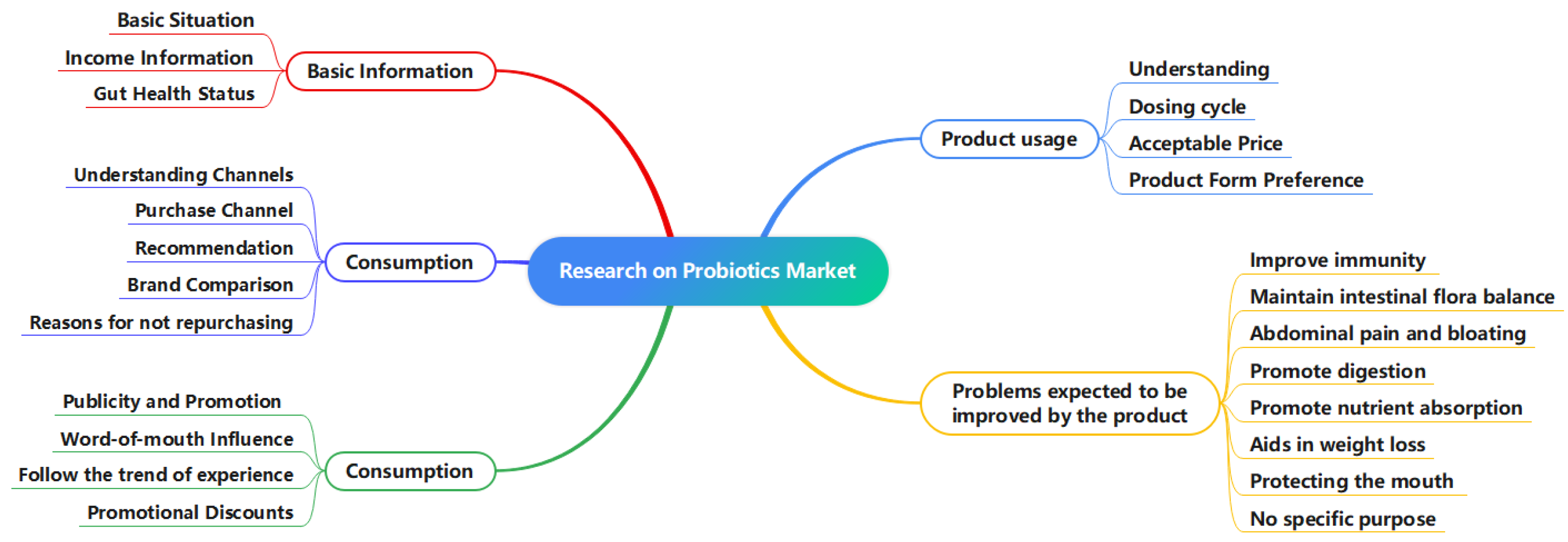
In this paper, we take probiotic products in marketing as an example by exploring the different preferences and behavioral patterns of consumers and clustering them in order to develop personalized marketing strategies. Through multi-dimensional analysis of consumers’ purchase history, preferences, needs, and other data, the designed spectral clustering algorithm based on graph comparison learning divides consumers into four categories: quality inspection communicator, pragmatists, healthy lifestyle consumers, and image ambassadors. On this basis, the customer profile is constructed to reveal the demand characteristics, preferences, and behavioral patterns of different consumer groups to help enterprises accurately grasp the target customer groups, so as to implement more targeted marketing measures. This not only helps companies optimize the allocation of marketing resources but also improves customer stickiness and promotes sales growth. In addition, building customer profiles would reveal the multi-method of consumer motivations in impulse repurchasing behavior.

This study provides an innovative solution for the node clustering problem in complex networks. As a practical application of complex network methods in marketing analysis, the main innovations of this paper are as follows:

• Optimizing the distance relationship between pairs of positive and negative samples in complex networks through contrastive learning, and automatically learning the deep-level feature representation of the data, so as to effectively improve the robustness of the model.
• When dealing with non-linearly divisible data, the similarity matrix between data points is utilized to map the high-dimensional data to the low-dimensional space to capture the global structure of the data, thus improving the accuracy of clustering.
• The model in this paper is especially capable of capturing the underlying structure that is difficult to discover by traditional methods when dealing with complex and heterogeneous data.

2. Related Works

With the rapid development of big data and artificial intelligence technology, research of clustering algorithms has been deepening, and clustering methods can be divided into various types according to their basic principles and applicable scenarios, such as clustering based on division, clustering based on density, and clustering based on deep learning.

2.1. Clustering Based on Division

Partition-based methods play an important role in clustering algorithms. In recent years, researchers have continuously explored new improvements and extensions to the traditional K-means algorithm in order to optimize clustering performance. Among them, Ran et al. proposed a novel K-means clustering algorithm based on a noise algorithm, in which the number of clusters is determined by randomly enhancing the attributes of the data points and the cluster centers are automatically initialized, thereby improving the accuracy and stability of clustering results [7]. Nie et al. reformulated the clustering objective function as a trace maximization problem, effectively addressing the issues of repeated calculation of cluster centers and slow convergence speed in the traditional K-means clustering algorithm [8].

Furthermore, with the development of deep learning technology, researchers have begun to combine deep learning methods with traditional partition-based approaches. For example, Yang et al. proposed an algorithm that combines autoencoders with K-means. This method pre-trains an autoencoder to map the input data into a low-dimensional space, and clustering is then performed in this space [9]. This hybrid clustering method, incorporating deep learning techniques, not only retains the simplicity and effectiveness of the traditional K-means algorithm but also improves clustering accuracy and generalization ability through deep learning. Seyed et al. proposed an improved fuzzy clustering algorithm based on the whale optimization algorithm, which addresses the issues of slow convergence and poor accuracy in traditional clustering methods when applied to large datasets by optimizing the initialization of cluster centers [10]. Huang et al. introduced a robust deep K-means model, which learns hidden representations related to different low-level attributes. This model uses deep structures to overcome the shortcomings of previous clustering methods in handling complex hierarchical information, thus enhancing clustering performance [11].

In summary, these methods form clusters by iteratively optimizing the distance between data points and cluster centers, making them suitable for most datasets with distinct cluster structures. With the integration of deep learning techniques, their clustering accuracy and generalization ability have been further improved, giving partition-based methods a greater advantage when dealing with high-dimensional and complex structured data.

2.2. Clustering Based on Density

Density-based methods cluster data points by calculating their local density and grouping them based on density values. The density peak clustering (DPC) algorithm, a representative example, assumes that cluster centers have high local density and are far apart, identifying them quickly through a decision graph [12]. Cheng et al. extended this by proposing an approximate spectral clustering algorithm based on dense cores and density peaks, using geographic distance and decision graphs to identify cluster centers, enabling the detection of complex structures and noisy data [13]. To address the performance limitations of traditional DPC when clusters with significant density differences are close, Fan et al. introduced an improved mutual density k-nearest neighbor graph [14]. Additionally, Chen et al. enhanced clustering efficiency by replacing traditional density calculations with a fast k-nearest neighbor algorithm [15]. Ding et al. proposed a density peak clustering algorithm based on a natural neighbor merging strategy (IDPC-NNMS), which adaptively calculates local density by identifying the natural neighbor set of each data point, effectively eliminating the impact of truncation parameters on the final results [16]. Rasool et al. introduced a similarity measure based on probabilistic mass and incorporated it into DPC, forming a data-dependent clustering algorithm [17]. Zhang et al. proposed an improved DPC algorithm based on balanced density and connectivity (BC-DPC), which introduced the concept of balanced density to eliminate density differences between clusters, accurately identify cluster centers, and ensure connectivity between data points and their nearest high-density points through mutual neighbor relationships, thus avoiding persistent clustering errors [18].

Guan et al. regarded clustering as a graph partitioning problem and proposed the main density peak clustering algorithm (MDPC+), which clusters by quickly detecting main density peaks in the peak graph and designing specific graph structures for non-peak and density peak points, enabling the reconstruction of clusters with complex shapes [19]. Yang et al. addressed the shortcomings of traditional DPC in similarity measurement, parameter selection, and local density calculation by defining divergence distance to evaluate data point similarity and determining key parameters based on an adjusted box plot theory, effectively identifying clusters of various shapes and spatial dimensions with minimal manual intervention [20]. Li et al. introduced a density peak clustering method based on fuzzy semantic units, converting each data point into a fuzzy semantic unit to define and estimate local density, addressing the challenge of accurately estimating local density in practical DPC applications [21]. Guo et al. tackled difficulties in center recognition and the “chaining effect” in DPC when handling non-spherical and non-uniform density clusters by incorporating connectivity estimation and a distance penalty mechanism [22]. Wang et al. proposed a pseudo-label guided density peak clustering algorithm (PLDPC), employing a pseudo-label generation method designed based on co-occurrence theory and avoiding manual parameter tuning through a mutual information maximization approach, achieving improved clustering results [23].

Overall, density-based methods can automatically identify clusters of any shape and exhibit good robustness to noisy data. These methods perform clustering by calculating the local density of data points and grouping them based on density values, effectively overcoming the limitations of traditional distance-based methods when dealing with non-spherical and unevenly distributed data. In recent years, various improvements have been introduced, which not only enhance the clustering accuracy and stability of density-based methods but also enable them to be applied to more complex and diverse datasets.

2.3. Clustering Based on Kernel

Kernel methods utilize kernel functions to map data to higher dimensional spaces and then perform linear clustering in these higher dimensional spaces. Xu et al. proposed the DKLM method, which designs a data-driven adaptive kernel learning mechanism to directly learn a kernel matrix satisfying the multiplicative triangle inequality constraint from data self-representation. This method addresses the limitations of traditional kernel methods, which rely on predefined kernels, struggle to preserve non-linear manifold structures, and assume an idealized affinity matrix. By maintaining local manifold structures in non-linear spaces and promoting block-diagonal affinity matrix generation, DKLM significantly enhances the robustness of clustering for complex data [24]. Xu et al. constructed a self-representation model for classification sequences, transforming clustering tasks in noisy environments into subspace clustering problems. This approach tackles the challenges of lacking effective similarity measures for sequence data and the interference of noise. By leveraging subspace methods to separate noise and extract latent structures, it achieves high-quality clustering for real-world data [25]. Wang et al. designed the LFMKC-PGR method based on multi-kernel clustering, which jointly learns kernel-based partitions and the subsequent fusion process. This approach addresses the issue of suboptimal solutions caused by the separation of kernel partitioning and fusion in multi-kernel clustering. By utilizing graph structures to capture complex relationships between kernels and optimizing partition consistency, the method further improves clustering performance [26]. These methods are very effective when dealing with non-linearly structured data.

2.4. Clustering Based on Deep Learning

In recent years, with the rapid development of deep learning technologies, methods based on deep learning have increasingly been proposed in the field of clustering algorithms. For instance, Caron et al. integrated deep learning with unsupervised clustering, employing an iterative approach to optimize feature learning and clustering simultaneously [27]. This approach not only enhances clustering accuracy and generalization capabilities but also provides new insights into the application of deep networks in unlabeled data scenarios. Hsu et al. addressed the clustering problem for large-scale unlabeled image datasets by proposing a CNN-based joint clustering and representation learning framework [28]. Yang et al. addressed the issue of reduced robustness in deep clustering methods under adversarial attacks by proposing a robust deep clustering method based on adversarial learning (ALRDC). This method defines adversarial samples in the embedding space and designs attack strategies, making it applicable to various existing clustering frameworks and significantly improving clustering performance [29]. Yang et al. proposed a recursive framework that jointly optimizes deep representation learning and image clustering. Through a recursive process, the framework integrates clustering algorithms with CNN output representations and employs a weighted triplet loss function to achieve end-to-end optimization. This significantly improves both the accuracy of image clustering and the generalization ability of the representations [30]. Yang et al. addressed the limitations of generative methods in clustering performance by proposing a model that combines hierarchical generative adversarial networks with mutual information maximization. Through theoretical analysis, it was demonstrated that mutual information maximization aids in the separation of clustering distributions in the data space. Various techniques were also employed to enhance the model’s stability and performance [31].

Recently, researchers have gradually introduced contrastive learning into graph data clustering tasks. Hassani et al. proposed the MVGRL method [32], a cross-view contrastive learning framework. This method extends the original adjacency matrix into a diffusion matrix, which is then used as both the local structural view and the global diffusion view of the graph. By optimizing the contrastive learning loss, MVGRL maximizes the cross-view mutual information between local node representations and global graph representations. This dual-view mutual information maximization strategy not only captures local neighborhood relationships at the node level but also integrates global topological features at the graph level. As a result, the learned node embeddings preserve local structural consistency while implicitly encoding global cluster distribution patterns, ultimately improving performance in node clustering tasks.

In addition to the aforementioned methods, researchers have also explored other deep learning-based clustering algorithms, such as structured deep clustering networks (SDCN) [33], deep robust clustering (DRC) methods [34], ClusterGAN [35], and adversarial graph autoencoders (AGAE) [36]. These deep learning-based methods automatically learn the latent representations of data through deep neural networks and apply them to clustering tasks, significantly improving clustering performance and generalization ability.

Deep learning-based methods can handle high-dimensional, non-linear, and complex data structures, and through iterative optimization of feature representations and clustering results, they achieve end-to-end clustering optimization. With the continuous advancement of deep learning technologies, these methods will demonstrate their powerful clustering capabilities in more fields. They not only improve clustering accuracy and stability but also enable applicability to more complex and diverse datasets, providing new solutions for data analysis and machine learning.

3. Materials

3.1. Data Collection and Analysis

This paper takes probiotic products in marketing as an example, and conducts data collection in the form of online and offline questionnaires for different consumer groups. A total of 1205 questionnaires were distributed in the formal survey of this study, and 1193 valid questionnaires were recovered, with a total recovery rate of 99%. The questionnaire was set up in five parts: basic information, use of probiotic products, problems expected to be improved by probiotics, consumption of probiotic series products, and influencing factors of purchase intention, with a total of 83 options. The structure of the questionnaire is shown in Figure 1.

Figure 1. The framework of the questionnaire for probiotic products.

In order to prevent questionnaire fatigue in respondents, we designed the scale questions in a variety of presentation formats to increase the interest of the questionnaire filling process. In order to exclude the influence of respondents’ lack of seriousness in answering on the data, we regarded the following two types of questionnaires as invalid questionnaires and excluded them:

• The questionnaire sets a lie detector question in the middle position, and those who answer this question incorrectly are regarded as invalid questionnaires;
• Questionnaires with a repetition rate of 85% or more for scale questions were considered invalid.

In this paper, we adopted the “Questionnaire Star” online questionnaire research method, which effectively avoided the problems of respondents’ missing answers and irregular answers. During the research process, we marked the questionnaires with low cooperation, fast filling speed, casual attitude, and giving up in the middle of the survey to ensure that the recovered valid samples are of high quality and that there are no missing or incomplete data. At the end of questionnaire distribution, the data were exported directly from the backend of the Questionnaire Star software, eliminating the need for manual entry, reducing the risk of error, and shortening the project implementation period.

Since the main purpose of the study is to improve the repurchase rate of probiotic products, this paper only focuses on the data analysis of the people who have used it—i.e., 547 out of 1193—to carry out the research.

3.2. Analysis of Factors for Consumer Persistence in Purchasing

The questionnaire selected 15 factors that may influence consumers’ purchasing decisions (as shown in Table 1), and classified the factors affecting consumers’ repurchase into four major categories, which are publicity and promotion factors, word-of-mouth influence factors, followers’ experience factors, and promotional discount factors.

Table 1. Statistical classification of goods that consumers continue to purchase.

Influencing Factors by Category	Subcategory
Publicity and Promotion Factor	Celebrities are using it
	Advertisement meets the demand
	Packaging design is clean and beautiful
Word-of-mouth Influence Factor	Main product, sales champion
	Recommended by sales staff
	Recommended by friends and family
	Recommended by bloggers, red books, etc.
Follower the Experience Factor	You should treat yourself better
	Peers are taking it
	Within your means
	Comparison
Promotional Discount Factor	Free Trial
	Specials
	Great Activities
	Reduced price and free gifts

• Factor 1: “Publicity and Promotion Factor”. This factor includes the use of celebrities and internet celebrities, the fit of the advertising campaign, and the aesthetics of the package design. These factors play a key role in customers’ continued purchase of the product. Recommendations from celebrities and Internet celebrities significantly increase brand awareness and consumer trust; while effective matching of advertising campaigns with consumer needs can trigger empathy and promote purchase decisions. In addition, clean and beautiful product packaging conveys the brand’s quality and professionalism. Together, these elements form a powerful promotional strategy that drives consumers’ continued purchasing behavior.
• Factor 2: “Word-of-Mouth Influence Factor”. This factor includes the attention generated by the main products and sales champions, recommendations from bloggers and social platforms such as Xiaohongshu, as well as recommendations from salespeople and friends and family. Main products and sales champions enhance consumers’ purchasing confidence by virtue of their market performance and recognition, while recommendations from bloggers and Xiaohongshu can quickly spread product information and profoundly influence potential consumers’ perceptions. In addition, recommendations from salespeople and friends and family often increase consumer trust due to their authority, and consumers tend to refer to real feedback from people around them. These factors together constitute the word-of-mouth influence factor, reflecting the degree of guidance and influence consumers receive when choosing and continuing to purchase a product.
• Factor 3: “Follow the Experience Factor”. This factor includes subcategories such as “you should be kinder to yourself”, “peers are taking it”, “within your means”, and “comparison” shopping. This factor is related to the environment around the consumer and reflects the extent to which the consumer will be influenced by their surroundings.
• Factor 4: “Promotional Discount Factor”. This factor covers factors such as free trials, special offers, discounts on various activities in various forms, and offers such as full price discounts and freebies. These factors reflect consumers’ sensitivity to product pricing and the impact of promotional activities on purchasing decisions.

4. Methodology

This study aims to detect potential user groups based on consumption characteristics in the probiotic market, gaining deep insights into consumers’ diverse preferences and behavioral patterns to formulate differentiated marketing strategies. The research found that user clusters generated by traditional clustering methods exhibit insufficient intra-cluster compactness and ambiguous inter-cluster separation. Contrastive learning, which maximizes similarity between positive sample pairs while minimizing similarity between negative sample pairs, aligns well with clustering objectives. Therefore, this paper employs a graph contrastive learning-based approach for user group clustering. The method first constructs a graph structure for discrete data using the KNN method, then performs pre-training through contrastive learning, and finally utilizes the trained representations for spectral clustering. This approach effectively enhances intra-cluster compactness and inter-cluster separation, enabling better identification of latent groups within sample data. The overall design framework of the algorithm is illustrated in the Figure 2.

Figure 2. The general design framework of the algorithm.

4.1. Construction of Users’ Graph

In many practical applications, there are inherent similarities or correlations between network nodes. KNN (K-nearest neighbor)-based graphs are able to capture these local similarities and provide the necessary structural information for graph-based learning algorithms. This graph structure can effectively capture the intrinsic geometric relationships of the data and provide important information about the similarity of the data points, which provides the necessary graph structure foundation for the subsequent graph convolutional network (GCN) and contrastive learning, and facilitates the subsequent deep learning models to perform more accurate clustering and analysis.

In this paper, the original user data collected are defined as $X\in R^{N\times d}$, where $x_i$ denotes the vector of attributes i of the user sample, N is the number of samples, and d is the dimension of the questionnaire. For each user sample, its top-K similar neighbors are first found to be similar to each other, and the edges are set to connect it to its neighbors, thus forming a complete graph structure G.

There are many ways to compute the sample similarity matrix $S\in R^{N\times N}$. This paper lists three methods commonly used to construct KNN graphs.

• Euclidean distance. The similarity between samples i and j is calculated as:

  $$S_{ij}={∥-x_i-x_j∥}^2$$

  (1)
  The method uses negative Euclidean distance as a similarity measure; the smaller the distance, the higher the similarity, and is suitable for use on data with consistent dimensional scales.
• Cosine similarity. The similarity between samples i and j is calculated as follows:

  $$S_{ij}={\displaystyle \frac{x_i·x_j}{∥x_i∥∥x_j∥}}$$

  (2)
  This method determines the similarity of two vectors by measuring their similarity in direction without considering their magnitude and is suitable for vector data.
• Dot product. The similarity between samples i and j is calculated as follows:

  $$S_{ij}=x_j^T{x}_i$$

  (3)
  The larger the dot product result calculated by this method, the more similar the two samples are, and it is applicable to any type of data.

After computing the obtained similarity matrix S, this paper selects the top-K similarities of each sample with its neighbors to construct an undirected k-nearest neighbor graph, which in turn obtains the adjacency matrix A from the non-graph data.The final obtained graph can be defined as $G=(A,X)$.

4.2. Data Augmentation and Encoding

After obtaining the graph G, in order to obtain richer sample node representations, this paper designs a self-supervised learning framework based on graph contrastive learning to train the data as a way to provide more reliable data support for formulating personalized marketing strategies. Among them, data augmentation is a key component of self-supervised learning, which is capable of generating samples with different features by performing various transformations on the original sample data, thus greatly enriching the diversity of the dataset.

Next, this paper utilizes an edge perturbation method to randomly add or subtract a certain percentage of edges to perturb the connectivity of the graph G, as a way of generating the two augmented views $G_1^{\prime }$ and $G_2^{\prime }$ needed for contrastive learning. This step is an effective graph data augmentation technique that can help the model learn a more generalized representation of the features, and improve its performance in the face of incomplete or noisy data.

After obtaining the two augmented views, in order to synthesize the sample data and the relationship between them during the training process, the encoder can adopt various network frameworks for encoding the data such as a graph neural network (GNN), graph attention network (GAT), etc. In this paper, we input two augmented views into the GCN to extract the node representations of the samples. The process of extracting node representations by the GCN can be defined as follows:

$$Z^{(k+1)}=\sigma \left(D^{-{\displaystyle \frac{1}{2}}}\widehat{A}{D}^{{\displaystyle \frac{1}{2}}}{Z}^{\left(k\right)}{W}^{\left(k\right)}\right)$$

(4)

where D is the degree matrix, $\widehat{A}=A+I$, I are the unit matrices, $Z^{\left(k\right)}$ is the node representation of the node of the kth layer, $W^k$ is the weight matrix of the kth layer, and $\sigma$ is the non-linear activation function.

For the node representations $Z_1$ and $Z_2$ obtained from the two augmented views, in order to improve the efficiency during the comparison learning training, this paper normalizes the two representations before performing the comparison loss in the following way:

$$Z_1^{\prime }={{\displaystyle \frac{Z_1}{∥Z_1∥}}}_2,Z_2^{\prime }={{\displaystyle \frac{Z_2}{∥Z_2∥}}}_2$$

(5)

Finally, the normalized node representations are fed into the contrastive learning framework for training.

4.3. Node Representation Based on Contrastive Learning

In traditional clustering methods, such as K-means or hierarchical clustering, these algorithms operate directly on the raw data in an attempt to group the inherent clusters found therein. However, these methods typically assume that the raw data used are divisible in feature space, which does not hold true in many real-world datasets. In addition, they do not utilize deep structural information between the data, which may result in clustering results that are not optimal. Contrastive learning, on the other hand, is able to learn richer and more discriminative feature representation by maximizing the similarity between positive sample pairs and minimizing the difference between negative sample pairs. This feature representation contains the deep structure and relationship between the sample data, which helps to improve the quality of the clustering.

Therefore, considering the limitations of traditional clustering methods, this paper does not directly use the node representations encoded by the GCN for clustering analysis, but first conducts training by using contrastive learning methods, so as to bring similar sample nodes closer and dissimilar sample nodes farther away, in preparation for the subsequent use of clustering methods. Specifically, in this paper, the nodes corresponding to each other in the two augmented views are regarded as a positive sample pair (e.g., $Z_{1i}^{\prime }$ and $Z_{2i}^{\prime }$ are positive sample pairs), with the remaining nodes regarded as negative sample pairs (e.g., $Z_{1i}^{\prime }$ and $Z_{2j}^{\prime }$ are negative sample pairs). The loss function for contrastive learning optimization can be expressed as follows:

$$\mathrm{L}=-log{\displaystyle \frac{exp\left(sim\left(z_{1\mathrm{i}}^{\prime }·z_{2i}^{\prime }\right)/\tau \right)}{exp\left(sim\left(z_{1i}^{\prime }·z_{2i}^{\prime }\right)/\tau \right)+{\sum }_{j\ne i}exp\left(sim\left(z_{1i}^{\prime }·z_{2j}^{\prime }\right)/\tau \right)}}$$

(6)

where $\tau$ is the temperature parameter. After these operations, the model is finally optimized by comparing the loss functions to train an encoder for subsequent clustering analysis.

4.4. Clustering of Users Based on Spectral Clustering

After training on the sample data, this paper uses spectral clustering to cluster the samples. The spectral clustering algorithm is based on graph theory, which considers the sample data points as the vertices of the graph and constructs the edges between the vertices by the similarity matrix. The algorithm achieves clustering by analyzing the eigenvectors of the Laplace matrix of the graph, which reveal the low-dimensional structure of the data.

Before performing spectral clustering, we use a trained encoder to obtain the final sample node representation. In this paper, the KNN is used to construct the similarity matrix S utilizing the new sample node representations:

$$S_{ij}=S_{ji}=\left\{\begin{array}{cc}0\hfill & x_i\notin \mathrm{KNN}\left(x_j\right)\mathrm{and}{x}_j\notin \mathrm{KNN}\left(x_i\right)\hfill \\ exp\left(-{\displaystyle \frac{\parallel x_i-x_j\parallel }{2{\sigma }^2}}\right)\hfill & x_i\in \mathrm{KNN}\left(x_j\right)\mathrm{or}{x}_j\in \mathrm{KNN}\left(x_i\right)\hfill \end{array}\right.$$

(7)

Afterwards, the similarity matrix S is used to approximate the adjacency matrix W of the graph, and then the Laplacian matrix L of the graph is computed from the obtained adjacency matrix:

$$L=D-W$$

(8)

where D is a degree matrix and the values on the diagonal are satisfied: $d_i={\sum }_{j=1}^N{w}_{ij}$.

Spectral clustering aims to find the eigenvectors $F\in R^{N\times k}$ corresponding to the first k eigenvalues of the smallest Laplacian matrix L, since these eigenvectors contain information about the clustering structure of the data and constitute a new feature space. The corresponding objective function is as follows:

$$mintr\left(F^{T}LF\right)s.t.F^{T}F=I$$

(9)

Finally, the sample data are clustered in these feature spaces using clustering algorithms such as K-means to obtain the final results. The clustering results not only reflect consumer preferences and behavioral patterns, but also provide an intuitive and actionable grouping basis for the development of personalized marketing strategies.

In summary, this paper synergistically optimizes representation learning with graph structure, thereby integrating contrastive learning with spectral clustering. Specifically, the contrastive loss function enforces the embedding space to exhibit a distribution characteristic of intra-class compactness and inter-class orthogonality by maximizing the similarity of positive sample pairs (augmented views of the same node) and minimizing the similarity of negative sample pairs (augmented views of different nodes). This aligns theoretically with the assumption of spectral clustering that the similarity matrix should have high intra-cluster connectivity and low inter-cluster connectivity. Furthermore, the introduction of local structural priors through KNN graph construction in the contrastive learning module effectively constrains the geometric properties of the embedding space. This ensures that the learned similarity matrix, when used to construct the Laplacian matrix in the spectral clustering stage, naturally carries clear cluster structure information in its top k smallest eigenvectors, thereby avoiding the eigenvector oscillation problem caused by the distortion of the original feature metrics in traditional spectral clustering.

5. Results and Discussions

5.1. Analysis of Clustering Results

The personalized clustering algorithm for probiotic users based on contrastive learning proposed in this paper takes the GCN model, which is commonly used in graph data networks, as the base network, combines it with the contrastive learning method to train on the sample dataset, and finally realizes the efficient clustering of the sample data. According to the results of the clustering analysis, the people who buy probiotics are divided into four categories, and we make a contrastive analysis of the influence factors corresponding to each category that affect repurchase. The experimental results are shown in Table 2, Figure 3 and the last row of Table 3:

Table 2. Clustering results of the algorithm in this paper.

Cluster Category	Frequency	Percentage (%)
cluster_1	68	12.43
cluster_2	345	63.07
cluster_3	45	8.23
cluster_4	89	16.27
Total	547	100

Figure 3. Distribution of different users in the four clusters. Among them, 1 corresponds to male and 2 corresponds to female in gender. Age is divided into six levels, corresponding to below 18 years old, 18–25, 26–30, 31–40, 41–50, and above 50 years old. Income is divided into six levels, corresponding to less than 3000 RMB, 3001–5000 RMB, 5001–10,000 RMB, 1001–20,000 RMB, 20,001–30,000 RMB, and more than 30,000 RMB. Occupations are divided into 10 categories: students, freelancers, teachers, business administrators, employees, service workers, worker laborers, retirees, state agencies/institutions, and other.

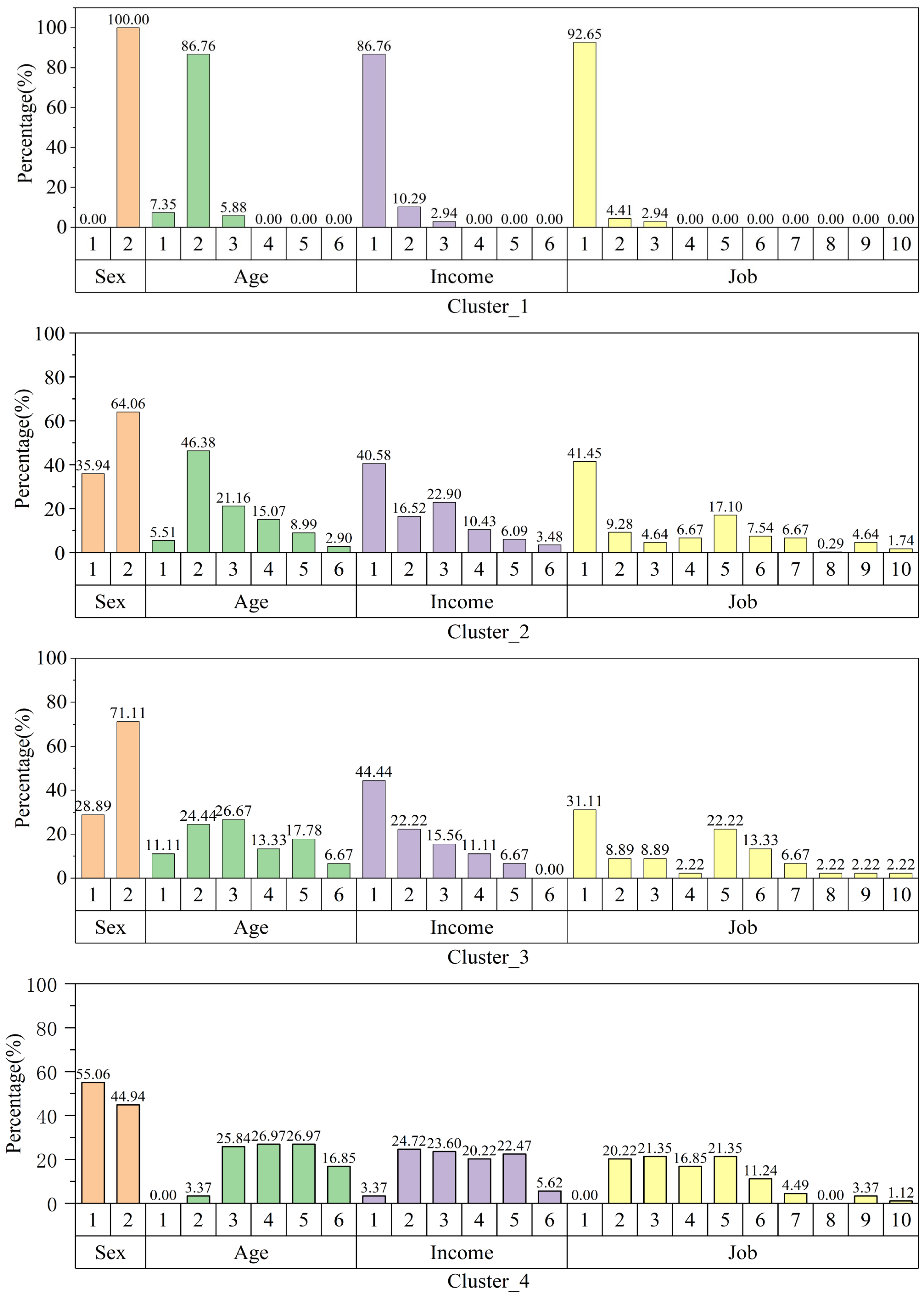
Based on the clustering results, we categorized the users into four groups as follows:

Cluster_1 accounts for 12.43% of the total sample, with a repurchase rate of 17.65%. They are mainly female students with low income, and their repurchase rate is the lowest in the total. The characteristics of this group of users are that they are sensitive to price, and perceive probiotics as a means to improve their perceived poor intestinal health. Their purchasing behavior is easily affected by external factors such as celebrity endorsements, advertising, and product promotions. They are more sensitive to price and pay more attention to product experience, such as the unique packaging appearance, carrying method, and eating method. In terms of probiotics efficacy, the speed of the efficacy will be a key factor influencing their purchasing behavior.

Cluster_2 accounts for 63.07% of the total sample, with a repurchase rate of 36.23%. The male-female ratio of this group is about 1:2. In terms of income, this group of users is significantly higher than cluster_1 and significantly lower than the other two groups of users. cluster_2 has the same sensitivity as cluster_1 to product prices. They are concerned about the medical effects of probiotics, hoping that probiotics could solve symptoms such as constipation, abdominal pain, and imbalance of flora. The external factors such as celebrity endorsements, advertising, and product promotions had no effect on the purchase decisions. However, the recommendations from relatives, friends, and technical bloggers would enhance their repurchasing rate.

Cluster_3 accounts for 8.22% of the total sample, with a repurchase rate of 55.56%. The ratio of men to women in this group is about 3:7, and the income level is similar to that of pragmatists. Although the two types of users are similar in terms of income level, this type of user is not sensitive to price. This type of user has the highest level of self-perception of intestinal health. In their opinion, probiotics should be an ordinary daily health diet product and represent a regular healthy lifestyle supplement that should be taken regularly. In addition, this type of user was also less affected by external factors such as celebrity endorsements, advertising, and product promotions. Friends, relatives, and technical bloggers recommending such light marketing methods would affect their purchasing behavior.

Cluster_4 accounts for 16.27% of the total sample, with a repurchase rate of 97.75%. The ratio of men to women in this group is about 5:4. The main occupations are freelancers, teachers, and business managers. The level of their income was the highest among the total sample. Similar to that of cluster_1, the purchasing behavior of this group was easily affected by external factors such as celebrity endorsements, advertising, and product promotions. Unlike the other groups, cluster_4 was not sensitive to price. In terms of product efficacy, this group has a strong sense of health and strongly agrees that probiotics are only taken as daily health products without a clear purpose. In terms of intake frequency, this type of user also has the highest intake frequency.

5.2. Comparative Analysis of Different Models

In order to compare the advantages of this model over other network models, this experiment is compared with the commonly used clustering algorithms—K-means, GMM (Gaussian mixture model), and SC (spectral clustering)—and the clustering effects of these methods after pre-training of contrastive learning are compared, respectively. In this experiment, 300 epochs are set uniformly when training the contrastive learning model, the k value is set to 6 or 10 when KNN constructs the graph structure, the learning rate is set to $5\times {10}^{-5}$ when the model is trained, and the weight_decay is set to $5\times {10}^{-4}$ by default. The experimental results are shown in Table 3:

Table 3. The clustering effect of different methods, where the values in the table are the repurchase rate of users in that cluster.

Methods	Cluster_1	Cluster_2	Cluster_3	Cluster_4
K-means	26.23%	29.46%	54.72%	73.63%
CL + K-means	30.47%	33.46%	53.45%	87.85%
GMM	23.35%	37.78%	64.13%	70.27%
CL + GMM	30.36%	32.52%	52.54%	87.29%
SC	12.64%	55.77%	69.05%	99.00%
CL + SC	17.65%	36.23%	55.56%	97.75%

Table 3. The clustering effect of different methods, where the values in the table are the repurchase rate of users in that cluster.

Methods	Cluster_1	Cluster_2	Cluster_3	Cluster_4
K-means	26.23%	29.46%	54.72%	73.63%
CL + K-means	30.47%	33.46%	53.45%	87.85%
GMM	23.35%	37.78%	64.13%	70.27%
CL + GMM	30.36%	32.52%	52.54%	87.29%
SC	12.64%	55.77%	69.05%	99.00%
CL + SC	17.65%	36.23%	55.56%	97.75%

As can be seen from Table 3, the modeling framework proposed in this paper enables the effectiveness of various commonly used clustering algorithms to be improved, even though there is a significant difference in the differentiation between clusters. For the K-means algorithm, the repurchase rate of Cluster_4 rises from 73.63% to 87.85%, further widening the differentiation from Cluster_3. For the GMM algorithm, on the other hand, after combining with the contrastive learning framework, the repurchase rate of Cluster_4 rises from 70.27% to 87.29%, which also makes the repurchase rate between the clusters significantly different. Although the SC algorithm obtains a higher repurchase rate for Cluster_4, there is little differentiation between Cluster_2 and Cluster_3. After training with contrastive learning, although the repurchase rate of Cluster_4 decreases, the differentiation between clusters is greatly improved. From the table, it can be seen that the clustering effect of the method of contrastive learning combined with spectral clustering is optimal, and the differentiation between each category is more significant.

To enhance the objectivity of performance evaluation, we introduce three internal clustering validation metrics: the silhouette coefficient (SC), the Calinski–Harabasz index (CHI), and the Davies–Bouldin index (DBI). These metrics can be calculated without the need for true labels, aligning with the unsupervised framework of this study. A detailed introduction is provided below:

The silhouette coefficient (SC) quantifies cluster separation by comparing each object’s similarity to its own cluster versus other clusters. |It is defined as follows:

$$SC={\displaystyle \frac{b\left(i\right)-a\left(i\right)}{max\left\{a\left(i\right),b\left(i\right)\right\}}}$$

(10)

where $a\left(i\right)$ is the average intra-cluster distance and $b\left(i\right)$ is the nearest inter-cluster distance. The SC ranges from [−1, 1], with higher values indicating stronger cluster cohesion and separation.

The Calinski–Harabasz index (CHI) evaluates cluster validity through the ratio of between-cluster dispersion to within-cluster variance. It is defined as follows:

$$CHI={\displaystyle \frac{tr\left(B_k\right)/\left(k-1\right)}{tr\left(W_k\right)/\left(n-k\right)}}$$

(11)

where $B\left(k\right)$ and $W\left(k\right)$ denote between-/within-cluster covariance matrices, k is the cluster count, and n is the sample size. Higher CHI values reflect better-defined clusters with maximized inter-cluster divergence.

The Davies–Bouldin index (DBI) measures cluster compactness by averaging maximal similarity between clusters. It is defined as follows:

$$DBI={\displaystyle \frac{1}{k}}\sum _{i=1}^k\underset{j\ne i}{max}\left({\displaystyle \frac{{\overline{d}}_i+{\overline{d}}_j}{d\left(c_i,c_j\right)}}\right)$$

(12)

where ${\overline{d}}_i$ is the average intra-cluster distance of cluster i, and $d\left(c_i,c_j\right)$ is the inter-cluster centroid distance. Lower DBI values (minimally 0) indicate optimal compactness and separation.

From Table 4, it can be observed that the proposed method demonstrates comprehensive advantages across three clustering metrics: it achieves the highest SC value, significantly outperforms most methods in CHI, and has the lowest DBI value among all methods. This indicates that the proposed model achieves an optimal balance in terms of intra-cluster compactness (SC), inter-cluster separation (CHI), and cluster structure clarity (DBI). Traditional graph autoencoder methods (such as GAE and VGAE) perform well in inter-cluster separation but slightly underperform in intra-cluster compactness and cluster structure clarity. Deep clustering methods (such as DAEGC and SDCN) perform poorly in inter-cluster separation. Contrastive learning methods (such as MVGRL) perform poorly across all three metrics, suggesting that using contrastive learning alone for clustering cannot clearly distinguish data categories. In contrast, the proposed method, through a joint optimization mechanism combining contrastive learning and spectral clustering, retains the ability of graph enhancement strategies to learn local neighborhood structures while reinforcing inter-cluster separability through global orthogonal constraints in the embedding space. This integrated strategy allows the model to simultaneously learn local features and global structures of data under complex data distributions, thereby achieving superior results in the metrics.

Table 4. Clustering effect of different methods.

Methods	SC	CHI	DBI
GAE [37]	0.62	4134.67	0.54
VGAE [37]	0.63	4326.37	0.48
SDNE [38]	0.56	2189.09	0.50
DAEGC [39]	0.59	1004.04	0.60
SDCN [33]	0.63	1030.09	0.50
MVGRL [32]	0.44	1549.79	0.67
Our	0.65	2886.88	0.42

Overall, it seems that the model proposed in this paper will be more accurate in analyzing the individual populations after clustering, can capture the nonlinear structure of the data, and is suitable for clusters with irregular shapes.

5.3. Parameter Sensitivity Analysis

In order to select the best value of k when constructing KNN graph, this paper has analyzed and compared the selection of k value of three methods, CL + K-means, CL + GMM, and CL + SC, and the results are shown in Figure 4.

Figure 4. Clustering effect of each method at different k values.

Overall, all three methods show some sensitivity to the choice of k. Among them, the repurchase rate from the clustering of CL + K-means shows a fluctuating upward trend with the increase in k and reaches the highest value at k = 3. The repurchase rate of CL + GMM shows a lower performance at k = 2 and k = 4, but gradually improves with the increase of k, and reaches the optimal value at k = 10. The repurchase rate of CL + SC shows a significant volatility for the change of k, especially in the vicinity of k = 6, where the repurchase rate rises dramatically and then levels off. This suggests that appropriately increasing the value of k usually helps to improve clustering performance, but the optimal choice of k may differ between methods and needs to be adjusted for specific applications.

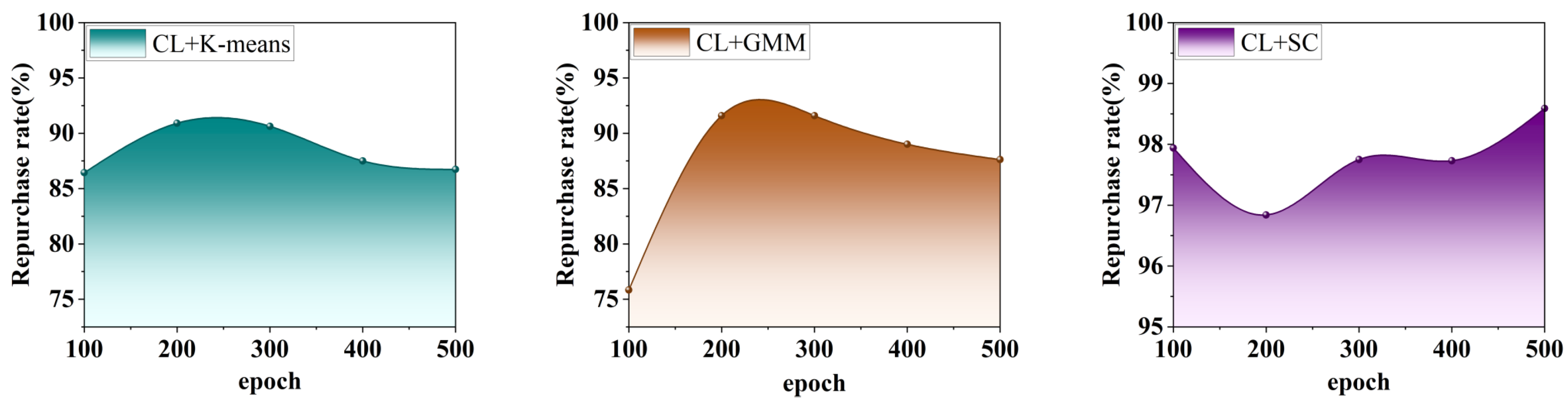
In addition, this paper also analyzes the trend in the repurchase rate in the clusters of the three methods under different numbers of training rounds (epoch = 100, 200, 300, 400, 500), and the experimental results are shown in Figure 5.

Figure 5. Clustering effect of each method at different epoch values.

As can be seen in Figure 5: At the initial stage (at epoch = 100), both CL + K-means and CL + GMM have relatively low repo rates. However, their performance rises rapidly as the number of training rounds increases, and begins to decline and stabilize after reaching the peak (around 300 epochs), suggesting that too much training may lead to performance degradation or overfitting. In contrast, CL + SC’s performance is more stable, maintaining high accuracy throughout all training rounds and improving slightly at a later stage (epoch = 500), suggesting that it is more robust to changes in training rounds. This result suggests that different methods should choose the number of training rounds appropriately to balance the convergence and performance of the model, where CL + SC is more suitable to maintain stable and higher performance in long-term training.

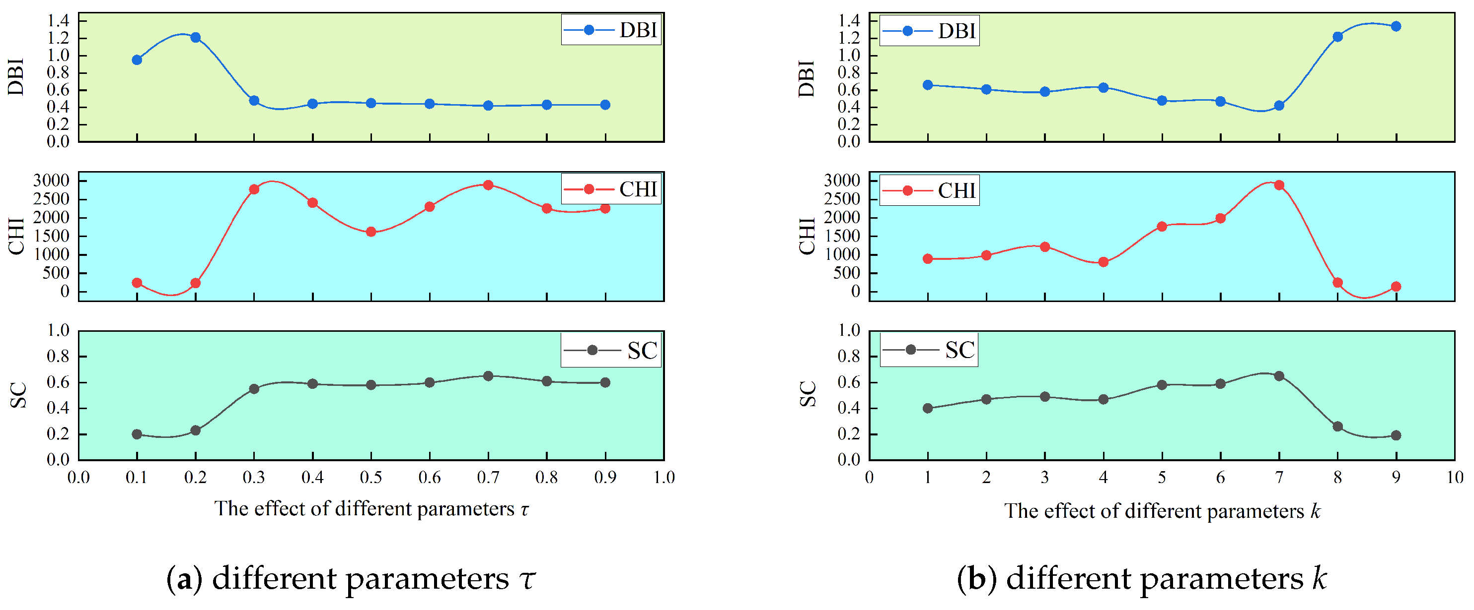
Through systematic adjustment of the temperature parameter $\tau$ in the contrastive learning loss function, we investigate its impact on node embedding quality and downstream spectral clustering performance. As shown in Figure 6a, as $\tau$ increases from 0.1 to 0.9, the silhouette coefficient (SC), the Calinski–Harabasz index (CHI), and the Davies–Bouldin index (DBI) exhibit distinct dynamic patterns.

Figure 6. The effect of different parameters.

In the low-temperature regime ($\tau =0.1$–$0.3$), model performance is severely constrained, indicating significant intra-class dispersion and inter-class overlap in the embedding space. A marked performance leap occurs at $\tau =0.3$, suggesting that moderate $\tau$ elevation effectively mitigates the contrastive loss sensitivity to hard negative samples. Within the intermediate temperature range ($\tau =0.4$–$0.6$), the model enters a stable optimization phase. Notably, all metrics simultaneously peak at $\tau =0.7$, demonstrating that this temperature setting optimally balances intra-class compactness and inter-class separability. Beyond $\tau =0.7$, performance marginally declines, indicating that excessive temperatures weaken the effectiveness of negative sample contrast.

Furthermore, we investigate the impact of the KNN graph construction parameter k on model performance. The k-value was selected from [1–9], with clustering quality comprehensively evaluated using the SC, CHI, and DBI, as detailed in Figure 6b.

At $k=1$, the model exhibits suboptimal performance due to graph fragmentation caused by sparse connections, which hinders effective neighborhood relationship capture. As k increases to 3, performance gradually improves, indicating that moderate neighborhood expansion enhances local structural awareness. Within the $k=5$–7 range, a substantial performance boost emerges, where enhanced graph connectivity facilitates global structural pattern discovery while suppressing noise interference. All metrics simultaneously peak at $k=7$, demonstrating that the KNN graph achieves an optimal equilibrium between local topology preservation and global structure representation, thereby providing an ideal foundation for subsequent contrastive learning.

However, performance degrades catastrophically when k exceeds 7. This collapse likely stems from over-densification of the graph structure, which forcibly connects dissimilar samples, blurs inter-class boundaries, and introduces spurious correlations. Our experiments conclusively establish that both excessively high and low k-values disrupt the model’s clustering compatibility, with $k=7$ identified as the optimal parameter.

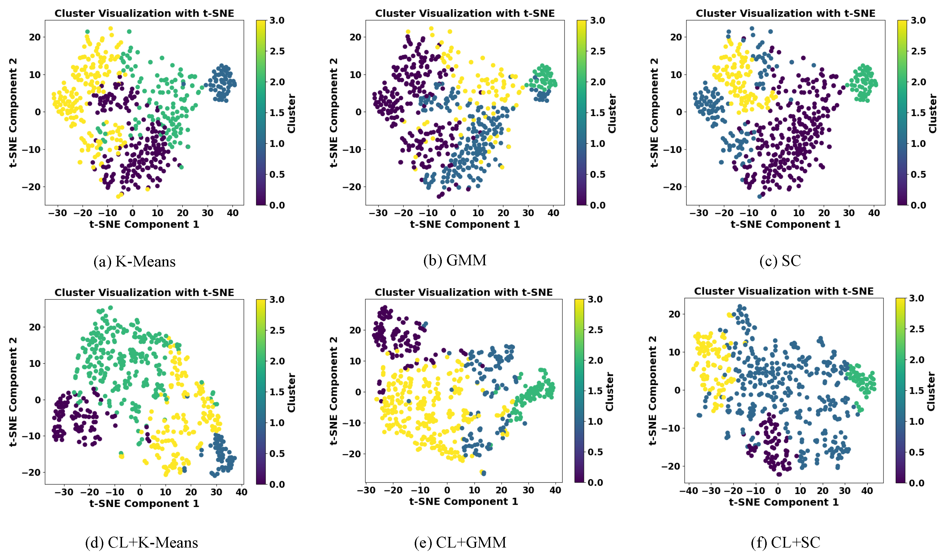
5.4. Visual Analysis of Clustering Results

Finally, this paper also visualizes and analyzes the clustering results of each method before and after adding contrastive learning, and the results are shown in Figure 7.

Figure 7. Clustering visualization of each method before and after adding contrastive learning.

From Figure 7, it can be clearly observed that after the dimensionality reduction processing of high-dimensional data, contrastive learning has a significant enhancement effect on the clustering effect of different methods. From Figure 7a, it can be seen that the clustering effect of K-means without adding contrastive learning is poor, the distribution of sample points is mixed, and the boundaries between the classes are not clear, while after adding contrastive learning (Figure 7d), CL + K-means significantly improves the clustering effect, and the separation between the classes is significantly improved. Figure 7b,e demonstrate the clustering results of GMM and CL + GMM, respectively. Among them, the GMM without adding contrastive learning has some class confusion, especially at the class boundaries, and the transition between classes is blurred; after adding contrastive learning, CL + GMM significantly improves the distribution of classes, with a higher degree of clustering of sample points in each class, and a clearer demarcation. Figure 7c,f then show the clustering comparison results of SC and CL + SC. Similar to the previous two methods, there is a partial overlap between the SC categories without adding contrastive learning, while after adding contrastive learning, CL + SC effectively enhances the intra-class compactness and inter-class separation, presenting an optimal clustering effect.

In summary, adding the contrastive learning module can make the data more clearly distributed in the space after dimensionality reduction and the boundaries between the categories more explicit, which can significantly enhance the effectiveness of different clustering methods.

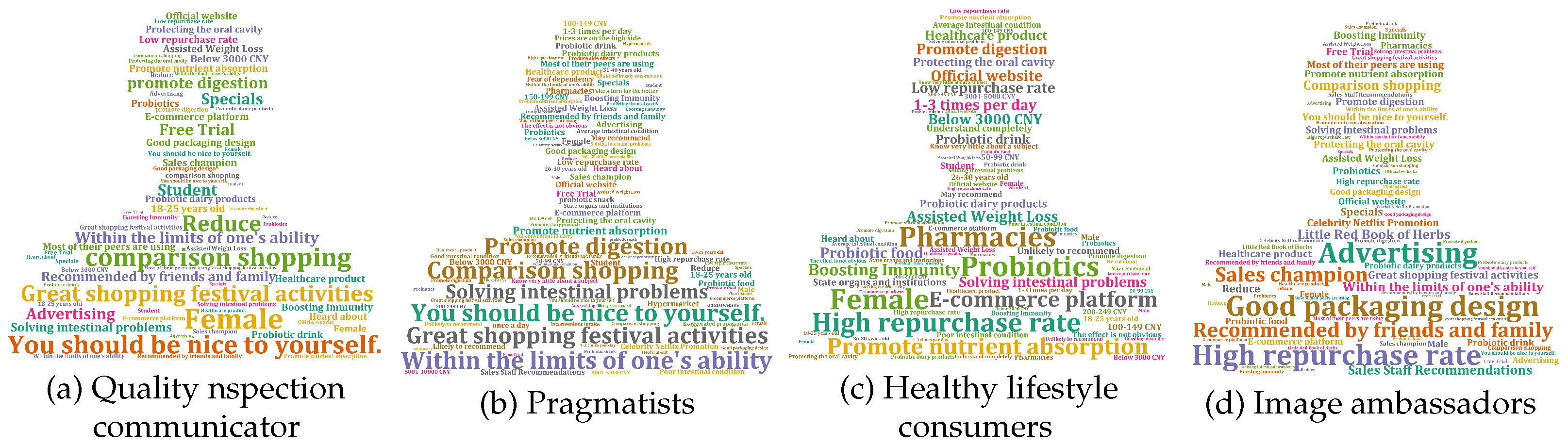
5.5. Visualization of User Profiling Results

In this paper, visualization tools were used to form a tag cloud of user profiles for purchasing probiotics and user profiles (e.g., Figure 8). Combining user’s purchasing intentions analysis matrix, the characteristics and interests of the consumer groups are intuitively described.

Figure 8. User profile tag cloud for Probiotics.

• Quality inspection communicator

Although purchase behavior of this type is influenced by brand marketing, product efficacy, product packaging, and product cost-effectiveness, which will compress the profit margin of the product, these users are the easiest to win over and their brand communication willingness is also the strongest compared with the other users. Quality inspection communicators are willing to share their own experience, thereby driving purchases among surrounding users. Without brand beliefs, this group possess an excellent ability to justify the quality of the probiotics and popularize them. Enterprises can accurately launch new products with high cost performance, seize the market, and expand the scope of their brand communication.

• Pragmatists

The repurchase behavior of this type of user was greatly affected by the efficacy and cost-effectiveness, and heavy marketing would not work for this type of user. In the cognition of this type of user, probiotics should have certain medicinal effects, can soothe the intestines, and need more technical product descriptions. Practical effects are what they care about most. This group accounts for the largest proportion of the overall sample, and its pragmatic attitude just shows that for most consumers, a good product is in itself a good advertisement.

• Healthy lifestyle consumers

The repurchase behavior of this type of user is affected by health habits. Compared with medicinal value, natural health status and healthy lifestyle are the core values they pursue. Therefore, advocating healthy life, green products, food safety, enhancing immunity, and high-quality life essentials are key to promoting consumption behavior in this type of user. Therefore, enterprises can target the characteristics of such users and build a joint brand and healthy ecosystem in daily home, kitchenware, fitness, and other scenarios by focusing on the essentials of healthy life and having international and domestic third-party food safety inspection certificates.

• Image ambassadors

Compared with other groups, the remarkable feature of this group of users is that they hope to improve their self-image through probiotics, such as taking probiotics to assist in weight loss and remove bad breath. In addition, as the group with the highest income level, this type of user has high requirements for the brand’s after-sale service and the speed of the product’s effectiveness. This type of user also has the highest repurchase rate among the overall group. For this type of user, brand image and periodic return visits are the focus of product marketing, and green weight loss and fresh breath should be the main features.

6. Conclusions

In complex network research, clustering analysis, as an effective exploratory tool for identifying different groups in a network and mining the interaction patterns among groups, can effectively reveal the potential relationship between nodes and the group structure in the network, so as to better understand the overall characteristics and local patterns of the system. In this paper, taking the market economy network as an example, combined with the analysis of consumer behavior, we propose a complex network node clustering model based on graph contrastive learning, which is used to deeply excavate user preferences and behavioral patterns. On this basis, a data-driven approach is used to build user profiles and formulate personalized market strategies. The model optimizes the distance relationship between pairs of positive and negative samples in a complex network by means of contrastive learning to automatically learn the deep feature representation of the data. At the same time, the similarity matrix between data points is utilized to capture the global structure of the data by mapping the high-dimensional data to the low-dimensional space, thus effectively improving the robustness of the model and the accuracy of clustering. The clustering model proposed in this paper is capable of identifying the underlying structure that is difficult to reveal by traditional methods when dealing with complex and heterogeneous data, providing profound theoretical support for optimizing decision-making, predicting behaviors, and formulating personalized strategies.

The methodology of this paper also has its limitations. The current implementation decouples contrastive learning and spectral clustering into sequential stages rather than a synergistic integration, and future research is planned to incorporate a new clustering loss that optimizes the node features along with the clustering objective. In addition, this paper uses a static KNN method to construct the graph, and in the future, we are ready to explore the method of adaptively adjusting the connection threshold according to the node density.