A Co-Optimization Method for Analog IC Placement and Routing Based on Sequence Pairs and Random Forests

Abstract

In the physical design of integrated circuits (ICs), conventional methodologies treat placement and routing as two sequential and independent steps, resulting in placement adjustments that do not sufficiently account for routing requirements. Such decoupled optimization leads to various routing challenges, including congestion and excessive wirelength. To address these limitations, we propose a novel iterative co-optimization framework that simultaneously considers placement and routing. Our methodology establishes an interdependent relationship between placement and routing, where routing is guided by the placement results and placement is adaptively adjusted based on the routing feedback. The proposed framework comprises two key components. First, we introduce an efficient gridless routing algorithm based on line exploration, which rapidly generates routing results by leveraging the placement state and netlist connectivity. The routing connectivity ratio and wirelength are then incorporated as the primary optimization metrics for placement refinement. Second, we develop an advanced placement optimization algorithm that integrates random forest techniques with Monte Carlo-based optimization. This algorithm systematically integrates routing information to guide iterative placement refinement, with the goal of achieving a higher routing connectivity ratio and a reduction in wirelength. We evaluated our approach on a dataset provided by Empyrean. Compared to the baseline placements in the dataset, the algorithm proposed in this work achieved an average improvement of 8.03% in terms of routing connectivity ratio and an average reduction of 18.33% in wirelength. Additionally, a comparative analysis of four optimization algorithms under the proposed co-optimization framework and the traditional half-perimeter wirelength (HPWL) method reveals achieved improvements of 12.41%, 14.16%, 13.87%, and 14.02% in the routing connectivity ratio, respectively, significantly outperforming the HPWL-based method. These results substantiate the efficacy of our co-optimization approach in enhancing IC physical design outcomes.

1. Introduction

With the rapid advancement in integrated circuit (IC) technology, the integration density of chips has been increasing significantly, imposing increasingly stringent demands on physical design. Placement and routing, as the core steps of physical design, critically influence chip performance, power consumption, area, and reliability. In the current IC physical design flow, placement and routing are typically performed separately: device placement is completed first, followed by routing. During the placement phase, the primary objectives are to optimize the chip area and half-perimeter wirelength (HPWL), aiming to reduce interconnect delay and power consumption.

To achieve these objectives, two main categories of methods are commonly employed: 1. Heuristic Algorithm Optimization: These methods draw inspiration from natural physical processes or biological evolution to perform stochastic searches within the design space, seeking optimal solutions that minimize area and HPWL. The common heuristic algorithms include simulated annealing [1], genetic algorithms [2], particle swarm optimization [3], and hybrid optimization [4]. 2. Reinforcement-Learning-Based Optimization [5,6]: This approach trains an intelligent agent to iteratively adjust device positions based on the current placement state and a reward function.

Area minimization aims to reduce chip costs, while HPWL minimization serves as an indirect metric for routing the connectivity ratio as a shorter HPWL typically implies lower routing congestion risk and helps to reduce the final wirelength. However, this separated design flow reveals significant limitations when applied to increasingly complex very large-scale integration (VLSI) designs. HPWL, as an estimate of wirelength, cannot accurately reflect actual routing paths or congestion conditions. Solely pursuing HPWL minimization often leads to severe congestion issues during the routing phase, resulting in a low routing connectivity ratio or excessive detours. The separation of placement and routing leads to frequent design iterations as issues identified during routing often require backtracking to the placement phase for adjustments. Such iterative processes are not only time-consuming and labor-intensive but can also lead to deviations from the optimal solution, ultimately impacting the performance and reliability of the chip.

To address these issues, this paper proposes a co-optimization method for placement and routing. This method recognizes the close interdependence between placement and routing, enabling the two steps to work collaboratively by optimizing placement based on routing feedback. We generate placements using a placement optimization algorithm and then perform routing using a line-exploration-based routing algorithm. The routing connectivity ratio and wirelength from the routing results are used as optimization objectives for iterative refinement. Additionally, we train a routability prediction model to filter out suboptimal placements, avoiding unnecessary routing and improving the optimization efficiency.

The main contributions of this paper are as follows:

1. We propose a placement and routing co-optimization method. By using a line-exploration-based routing algorithm for fast routing, the routing results are incorporated into the placement optimization objective function. This allows the placement phase to promptly incorporate routing feasibility information, ensuring that placement adjustments better align with the routing requirements and reducing the subsequent routing iteration time.

2. We propose a placement optimization algorithm that combines random forest and Monte Carlo optimization. First, a random forest algorithm is used to construct a routability prediction model to estimate the routing connectivity ratio of placement solutions. This model is then integrated with Monte Carlo optimization to guide placement refinement, effectively improving the routing connectivity ratio, reducing wirelength, and accelerating the optimization process.

3. The effectiveness of the proposed method has been experimentally validated. We evaluated our approach on a dataset provided by Empyrean. Compared to the baseline placements in the dataset, the algorithm proposed in this work achieved an average improvement of 8.03% in routing connectivity ratio and an average reduction of 18.33% in wirelength. Furthermore, we compared the performance of four optimization algorithms under the proposed co-optimization method and the traditional HPWL-based method. The results demonstrate that the four algorithms under the co-optimization framework outperformed the HPWL-based approach, achieving improvements of 12.41%, 14.16%, 13.87%, and 14.02% in terms of the routing connectivity ratio, respectively.

2. Related Work

As the technology nodes of very large-scale integration (VLSI) continue to shrink, placement optimization has become a critical step in the VLSI design flow. Efficient placement strategies not only reduce signal wirelength and routing congestion but also enhance the overall performance of chips. Therefore, designing efficient placement optimization algorithms has always been a research focus in the field of VLSI design. Traditional VLSI design flows separate placement and routing into two independent stages. During the placement stage, the primary goal is to optimize the positions of cells to minimize the chip area and the half-perimeter wirelength (HPWL) of signal interconnects. To address this complex optimization problem, researchers have proposed various heuristic algorithms, such as simulated annealing [7], genetic algorithms [8], parallel particle swarm optimization [9], and hybrid optimization [10]. These heuristic algorithms often rely on manually designed heuristic rules and, while achieving good results in specific scenarios, struggle to adapt flexibly to evolving design requirements and complex constraints.

2.1. Placement Methods

With the rise of artificial intelligence (AI) technologies, reinforcement learning (RL) has gradually been introduced into VLSI placement optimization. Azalia M et al. [11] proposed a deep-reinforcement-learning-based method for chip floorplan design, which generates floorplans that outperform or match manually designed ones in key metrics such as power consumption, performance, and chip area. Lai et al. [12] proposed an innovative deep reinforcement learning method called MaskPlace, which transforms the chip placement problem into a pixel-level visual representation learning task and solves it using convolutional neural networks (CNNs). Yu, S et al. [13] proposed a sequence-pair-based deep reinforcement learning placement algorithm where an RL agent explores the search space within sequence pairs and iteratively selects candidate neighbor solutions to optimize placement. RL learns optimal policies through interaction with the environment, automatically adjusting cell placements to optimize the objective function. However, applying RL to VLSI placement still faces numerous challenges, including the enormous scale of state and action spaces, the complexity of reward function design, and training efficiency issues.

2.2. Placement and Routing Co-Optimization Methods

In recent years, the co-optimization of placement and routing has gradually become a research hotspot. Huang et al. [14] proposed a co-optimization algorithm that leverages R-tree-based fast preprocessing and incorporates global routing information after global placement, combined with a breadth-first search (BFS)-based three-dimensional approximate addressing algorithm to optimize detailed placement. This method aims to select optimal cell movement positions to reduce total wirelength and improve routing connectivity ratios while further optimizing routing paths through partial rerouting techniques. Wang et al. [15] proposed that the Starfish engine achieves co-optimization of placement and routing by integrating cell movement and A*-algorithm-based partial rerouting strategies. This approach effectively bridges the gap between the traditionally separated placement and routing stages, reducing global routing wirelength. However, such methods typically consider routing information only after completing global placement, failing to fully utilize routing information early in the placement stage.

Unlike previous work, the algorithm proposed in this work innovatively introduces global routing information during the global placement stage, guiding global placement optimization through feedback from global routing. By employing this co-optimization approach, placement and routing information are effectively integrated at the early design stage, enabling simultaneous optimization of key metrics such as wirelength and routing connectivity ratio during global placement. Compared to traditional placement-routing separation methods, this strategy can identify and address potential routing congestion issues earlier, further enhancing the performance and manufacturability of IC chips.

3. Problem Formulation

Given a placement L, a netlist N, a set of pins P, and a multi-layer Analog IC of the placement region M, where the placement $L=\{m_1,m_2,\cdots ,m_n\}$ consists of n device modules, each module $m_i$ ($0\le i\le n$) has a corresponding shape and size; the netlist information $N=\{n_1,n_2,\cdots ,n_k\}$, where each net contains two or more pins to be connected; i.e., $\forall n_i\in N$ ($0\le i\le k$), $n_i=\{p_1,p_2,\cdots ,p_j\}$ ($j\ge 2$, $p_j\in P$). The goal of placement and routing co-optimization is to place device modules reasonably within the placement region M while performing routing, using the routing results as objectives for placement optimization, to maximize the routing connectivity ratio (RCR) and minimize the total wirelength, thereby generating an excellent placement.

The placement constraints C consist of two aspects: boundary constraints and non-overlap constraints, Specifically, the boundary constraints guarantee that all modules remain within the placement region, while the non-overlap constraints prevent any two modules from occupying the same space. Together, these constraints define the feasible solution space for the optimization problem.

Boundary Constraints: Each module $m_i$ must be entirely located within the placement region. Let the width of the placement region be $w_X$, the height be $h_Y$, and the bottom-left corner coordinates of module $m_i$ be $(x_i,y_i)$, with length $l_i$ and width $w_i$. The boundary constraints can be expressed as

$$\forall m_i\in L:\left\{\begin{array}{cc}{x}_i+l_i\le w_X,\hfill & 0\le x_i\hfill \\ y_i+w_i\le h_Y,\hfill & 0\le y_i\hfill \end{array}\right.$$

(1)

Non-Overlap Constraints: Any two distinct modules $m_i$ and $m_j$ must not overlap. This can be expressed as

$$\forall i,j(i\ne j):\left\{\begin{array}{c}(x_i+l_i\le x_j)\vee (x_j+l_j\le x_i)\hfill \\ (y_i+w_i\le y_j)\vee (y_j+w_j\le y_i)\hfill \end{array}\right.$$

(2)

The routing connectivity ratio (RCR) is generally defined as the ratio of the number of successfully routed connections to the total number of connections. A higher RCR implies greater reliability in circuit functionality. The RCR is calculated as shown in the following equation:

$$RCR\left(L\right)={\displaystyle \frac{p^{\prime }}{p}}\times 100\%$$

(3)

where p is the total number of pin pairs, and $p^{\prime }$ is the number of successfully connected pin pairs.

The total wirelength is another important metric for evaluating routing quality, reflecting signal transmission delay and power consumption. The total wirelength is calculated by summing the lengths of all segments in each net. The formula is as follows:

$$WL\left(L\right)=\sum _{i=1}^k\sum _{e\in E\left(n_i\right)}length\left(e\right)$$

(4)

where $E\left(n_i\right)$ represents the set of segments in the routing path of net $n_i$, and $length\left(e\right)$ represents the length of segment e.

Our objective function is to maximize the routing connectivity ratio and minimize the wirelength under the constraints C, as shown in the following formula:

$$\left\{\begin{array}{cc}\mathrm{Maximize}\hfill & RCR\left(L\right)\hfill \\ \mathrm{Minimize}\hfill & WL\left(L\right)\hfill \\ \mathrm{s}.\mathrm{t}.\hfill & \mathrm{C}\hfill \end{array}\right.$$

(5)

4. Placement and Routing Co-Optimization Method Based on Routability Prediction

This paper proposes a placement and routing co-optimization method that tightly integrates placement and routing algorithms to iteratively improve placement quality. Specifically, during the placement phase, the sequence pair algorithm is used to generate multiple placement solutions, ensuring that they satisfy placement constraints. During the routing phase, these placement solutions are routed, and the routing results are fed back. To improve efficiency, this paper employs a random forest algorithm to train a routability prediction model based on placement features, which is used to pre-filter placements with poor routing connectivity ratios. In the co-optimization process, the placement algorithm continuously adjusts the sequence pairs based on feedback from the routing results. In each iteration, multiple new placement solutions are generated, and the routability prediction model filters out placements with poor routing connectivity ratios. The remaining new placement solutions are compared with the current optimal placement in terms of routing results. If a new placement outperforms the current solution in routing metrics, the system updates the optimal solution. Through this multi-round iterative process, the placement quality is gradually improved, ultimately yielding high-quality placement and routing results. The overall co-optimization framework is illustrated in Figure 1.

4.1. Placement and Routing Co-Optimization

To fully leverage the advantages of placement and routing co-optimization, this paper designs an iterative co-optimization method based on the Monte Carlo algorithm and a routability prediction model. This method starts with an initial Analog IC placement and constructs an action search space by defining a series of placement transformation actions. Additionally, we design an evaluation function that comprehensively considers routing connectivity ratio (RCR) and wirelength to quantify the quality of placements. Unlike traditional methods, after each placement adjustment, we use a pre-trained random forest model to evaluate the routability of the routed placement, filtering out inferior placements. Simultaneously, the Monte Carlo algorithm probabilistically selects placements for routing attempts, and the placement is optimized based on feedback from the routing results. This paper employs the sequence pair algorithm for global search, exploring the solution space by adjusting module positions to find the optimal solution. To enhance optimization efficiency, we introduce a routability prediction model based on random forests, which filters out layouts with low routing connectivity ratios, thereby focusing resources on exploring high-quality solution regions and achieving local search. However, overly strict filtering may cause the algorithm to converge prematurely to a local optimum. To address this, we incorporate the Monte Carlo algorithm, which probabilistically selects layouts with lower routing connectivity ratios for exploration, ensuring that the algorithm can search within a broader solution space and avoid becoming trapped in local optima.

The connectivity between modules in the Analog IC layout is determined by netlist information. As a result, any changes in placement directly influence routing outcomes. To address this, we conduct a routing evaluation after each placement adjustment and integrate the routing results into the placement optimization process. The current placement is updated only if the evaluation function of the routed placement is superior to that of the current placement. This approach ensures that each optimization step leads to measurable improvements in routing performance. The iterative cycle of placement, routing, evaluation, and optimization allows the placement optimization process to comprehensively account for the impact of routing, thereby avoiding the suboptimal solutions frequently observed in traditional methods due to the decoupling of placement and routing. The algorithm iterates until convergence criteria are satisfied (reaching the maximum number of iterations), ultimately producing an Analog IC layout that adheres to design constraints and demonstrates optimal routing performance.

To achieve the dual objectives defined in Equation (5) (maximizing RCR and minimizing wirelength) while prioritizing the optimization of the routing connectivity ratio, we treat the minimization of wirelength as a secondary objective to the maximization of the routing connectivity ratio. By transforming the multi-objective optimization problem into a single-objective function, we have designed the following unified objective function:

$$F\left(L\right)=RCR\left(L\right)+{\displaystyle \frac{\partial }{WL\left(L\right)}}$$

(6)

where $RCR\left(L\right)$ represents the routing connectivity ratio of placement L, ranging from 0 to 1; $WL\left(L\right)$ represents the total wirelength of placement L; and ∂ is a weighting coefficient that adjusts the relative importance of RCR and wirelength in the objective function. In this formula, we prioritize optimizing RCR while also considering wirelength as a secondary objective. A smaller $WL\left(L\right)$ results in a larger ${\displaystyle \frac{1}{WL\left(L\right)}}$, which, when combined with $RCR\left(L\right)$, allows for simultaneous optimization of routing connectivity ratio and wirelength.

Since the placement algorithm we use is the sequence pair algorithm (which encodes the relative positional relationships between all modules by defining two linear sequences), we need to extract module information (length and width of each module) from the initial placement and initialize the sequence pairs (generated by randomly permuting module indices). This information is then passed to the placement algorithm, which generates placements based on the sequence pairs and module information.

To improve the efficiency of placement optimization, we introduce a routability prediction model. This model, based on the random forest algorithm, is trained using placement features and can predict the routing connectivity ratio of a given placement, filtering out placements with poor routability. We set the threshold of the routability prediction model to $\gamma$. Placements with predicted RCR below $\gamma$ are labeled as 0 (unroutable), while those above $\gamma$ are labeled as 1 (routable). To prevent situations where all new placements are labeled as unroutable due to the threshold $\gamma$ (causing the objective function values of both the current and new placements to fall below the threshold), we introduce the Monte Carlo algorithm. During placement selection, the probability formula $P\left(L\right)$ determines whether routing is performed. The formula for $P\left(L\right)$ is as follows:

$$P\left(L\right)=\left\{\begin{array}{cc}1-{\displaystyle \frac{1}{1+e^{k\left(F\right(L)-\gamma )}}},\hfill & H\left(L\right)=0\hfill \\ 1,\hfill & H\left(L\right)=1\hfill \end{array}\right.$$

(7)

where $\gamma$ is the classification threshold, k is a tuning parameter, and $H\left(L\right)$ is the prediction result. Since $H\left(L\right)$ is either 0 or 1, if $H\left(L\right)=1$, the placement is directly routed; if $H\left(L\right)=0$, the probability formula $P\left(L\right)$ determines whether routing is performed. The value of $P\left(L\right)$ depends on the relationship between the objective function value $F\left(L\right)$ of the current placement L and the threshold $\gamma$. The lower the objective function value relative to the threshold, the greater the need to find optimizable targets from candidate placements, making it more likely to accept new candidate placements for routing.

Placement and Routing Co-Optimization Flow

• Initial Placement Generation: Since the initial placement significantly impacts subsequent placements, we initialize n sequence pairs, route the n placements returned by the placement algorithm, and select the placement with the maximum $F\left(L_i\right)$ as the initial placement $L_{\mathrm{initial}}$.

  $$L_{\mathrm{initial}}=arg\underset{L_i}{max}F\left(L_i\right),i=1,2,\cdots ,n$$

  (8)
• Candidate Placement Generation: Based on the initial placement $L_{\mathrm{initial}}$, generate N new candidate placements $L_1,L_2,\cdots ,L_N$ by adjusting the placement using the placement algorithm.
• Feature Extraction and Prediction: For the generated N candidate placements, extract their placement features, construct a feature matrix, and input it into the prediction model. Features include module dimensions, positions, and pin locations. The prediction model, based on the random forest algorithm, outputs the prediction result $H\left(L_i\right)$ for each placement.
• Routing Decision: Use the probability formula $P\left(L_i\right)$ to determine whether routing is needed for placement $L_i$. Generate a random number r ($0<r<1$). If $r>P\left(L_i\right)$, perform routing, and calculate the routing connectivity ratio and wirelength to generate the objective function value.
• Placement Evaluation and Update: To improve efficiency, introduce an early stopping strategy. For each generated candidate placement $L_{\mathrm{new}}$, if $F\left(L_{\mathrm{new}}\right)\le F\left(L_{\mathrm{initial}}\right)$, continue evaluating the next candidate placement. If $F\left(L_{\mathrm{new}}\right)>F\left(L_{\mathrm{initial}}\right)$, stop evaluating subsequent candidate placements with probability $P_{\mathrm{stop}}\left(L_{\mathrm{new}}\right)$ and update the initial placement $L_{\mathrm{initial}}=L_{\mathrm{new}}$, proceeding to the next iteration. The formula is as follows:

  $$P_{\mathrm{stop}}\left(L_{\mathrm{new}}\right)={\displaystyle \frac{1}{1+e^{k(F\left(L_{\mathrm{new}}\right)-\gamma )}}}$$

  (9)

  where $\gamma$ is the classification threshold, and k is a tuning parameter.
• Iteration: Repeat steps 2–5 until the maximum number of iterations T is reached.

The overall algorithm is shown in Algorithm 1.

Algorithm 1 Placement Optimization Algorithm

1: Initialize placement L 2: Load routability model P 3: Set maximum number of iterations T 4: Set batch size N 5: Randomly select actions to initialize multiple placements and update L with the best placement 6: for $t\in T$ do 7:     Initialize the current batch placement list $L_{\mathrm{list}}$ 8:     for $n\in N$ do 9:         Apply placement transformation to L to generate a new placement $L^{\prime }$ 10:       Extract placement features and store them in $L_{\mathrm{list}}$ 11:   end for 12:   Use the routability model P to predict $L_{\mathrm{list}}$ and obtain $y_{\mathrm{pred}}$ 13:   for $n\in N$ do 14:         if $\mathrm{Random}(0,1)>P\left(L\right)$ then 15:            if $F\left(L_{\mathrm{list}}\left[n\right]\right)>F\left(L\right)$ then 16:                Update placement L 17:                if $\mathrm{Random}(0,1)>P_{\mathrm{stop}}\left(L\right)$ then 18:                    Break 19:                end if 20:            end if 21:         end if 22:    end for 23: end for

This study constrains the global search scope by defining a maximum iteration count T, thereby avoiding excessive computational overhead. To refine local search efficiency, a routability prediction model filters out placement solutions with low routing connectivity ratios, narrowing the optimization space. The time complexity of the random forest prediction is $O(d·k)$, where d represents the depth of each decision tree and k is the number of trees in the forest. This ensures efficient filtering while maintaining high accuracy.

To enhance robustness, a Monte Carlo-based probabilistic mechanism (Equation (7)) is introduced, allowing partially filtered layouts to participate in routing attempts with probability $P\left(L_i\right)$, mitigating the risk of discarding high-quality solutions due to overly strict model thresholds. The line-exploration-based routing algorithm is then applied to evaluate the routing feasibility of the remaining placements. The time complexity of this routing algorithm is $O(p·m)$, where p is the number of pin pairs and m is the number of modules. This approach avoids the grid mapping process, significantly reducing the search space and improving efficiency.

The sequence pair algorithm is used to generate and adjust candidate placements, with a time complexity of $O\left(n^2\right)$, where n is the number of modules. This complexity arises from the longest common subsequence (LCS) computation during the decoding process.

By combining these components, the overall time complexity of the co-optimization framework can be expressed as $O(T·N·(O\left(n^2\right)+O(d·k)+O(p·m)))$, where T is the maximum number of iterations, N is the number of adjustments per iteration, $O\left(n^2\right)$ corresponds to the sequence pair generation and adjustment, $O(d·k)$ reflects the random forest prediction, and $O(p·m)$ accounts for the line-exploration-based routing. This structured approach ensures efficient exploration of the solution space while balancing computational cost and optimization quality.

Concurrently, an early stopping strategy (Equation (9)) dynamically evaluates local optimization progress: when the objective function value increases, terminate the current search batch in advance with probability $P_{\mathrm{stop}}\left(L_{\mathrm{new}}\right)$ to further improve optimization efficiency.

4.2. Placement Algorithm

The core objective of this chapter is to generate new placement solutions by adjusting module positions, thereby exploring the solution space and identifying high-quality design outcomes. Among the various placement algorithms, such as the Sequence Pair algorithm, O-Tree algorithm [16], and B*-Tree algorithm [17], the sequence pair algorithm is widely adopted for solving integrated circuit placement problems due to its flexibility and efficiency. By encoding the relative positional relationships between modules, this algorithm can rapidly generate legal placement solutions within a constrained search space. Therefore, this paper selects the sequence pair algorithm as the primary method for modifying placements, leveraging its capability to efficiently explore the solution space and produce high-quality placement solutions that satisfy design constraints.

The sequence pair algorithm is a highly flexible method for describing placement structures. It is a topological representation that is independent of the sizes of circuit modules and only reflects the relative positional relationships between them. The core idea of the sequence pair representation is to use two sequences, positive and negative, composed of module indices to represent their geometric relationships. Given a sequence pair, we can derive the positional relationship graph between modules, thereby obtaining a specific placement.

Murata et al. [18] revealed the properties of relative positions between modules in a sequence pair. For any two modules $a_i$ and $a_j$ in a sequence pair $\langle T^{+},T^{-}\rangle$, there are four possible relationships:

• If $a_j$ appears after $a_i$ in both $T^{+}$ and $T^{-}$, then $a_i$ is to the left of $a_j$.
• If $a_j$ appears before $a_i$ in both $T^{+}$ and $T^{-}$, then $a_j$ is to the right of $a_i$.
• If $a_j$ appears before $a_i$ in $T^{+}$ but after $a_i$ in $T^{-}$, then $a_j$ is below $a_i$.
• If $a_j$ appears after $a_i$ in $T^{+}$ but before $a_i$ in $T^{-}$, then $a_i$ is above $a_j$.

Tang et al. [19] proposed a fast longest common subsequence (fast LCS) algorithm to convert a sequence pair into a placement. The algorithm uses the weight of each module on the x-axis (i.e., the module’s length) and the weight on the y-axis (i.e., the module’s width), along with the sequence pair, to determine the x and y coordinates of each module.

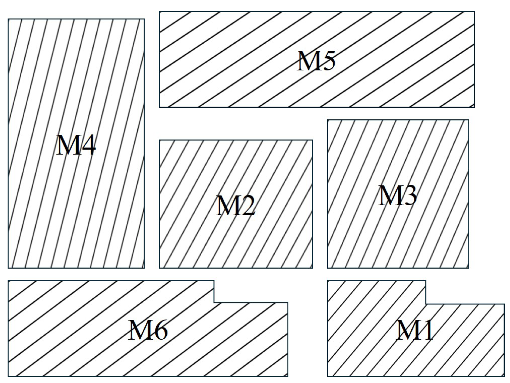
For any module a in the sequence pair $(X,Y)$, if its arrangement in the sequence pair is $(X_{1}a{X}_2,Y_{1}a{Y}_2)$, then the x-coordinate of module a is the sum of the lengths of the modules corresponding to the longest common subsequence of $(X_1,Y_1)$, and the y-coordinate is the sum of the widths of the modules corresponding to the longest common subsequence of $(X_2^R,Y_1)$. Here, $X_2^R$ is the reverse sequence of $X_2$. To facilitate subsequent routing, this paper sets the module spacing to 10 units and selects 6 modules to generate a sequence pair for demonstration. The placement result is shown in Figure 2.

The core idea of the sequence pair lies in using two sequences to encode the relative positions of modules, where each sequence is a permutation of all module indices. In the co-optimization method, the initial sequence pair is generated by randomly permuting the module indices of the placement, and then the LCS algorithm is used to decode it into a placement. After initialization, the placement is adjusted by incrementally selecting actions. Since changes in module positions within the sequence pair affect the overall placement, adjustments to module dimensions (length and width) will correspondingly alter the placement, and flipping a module will change its pin positions. Given that the netlist connectivity is fixed, changes in placement and pin positions will impact the routing connectivity ratio. Therefore, in the proposed algorithm, we define the following four actions for adjusting the sequence pair:

• Randomly swap two modules in the positive sequence.
• Randomly swap two modules in the negative sequence.
• Randomly swap the length and width of a module.
• Randomly flip a module.

In layout constraints, all modules must satisfy two basic conditions: modules must not overlap, and they must not exceed the layout boundary. The sequence pair avoids module overlaps by defining relative positions to determine coordinate information. However, random adjustments to the sequence pair may cause modules to exceed the layout boundary. Therefore, we need to filter these sequence pairs to ensure the legality of the layout. Illegal sequence pair filtering focuses on the construction of the initial sequence pair and adjustments to the sequence pair during layout modifications. The specific implementation steps are as follows:

Coordinate Calculation: Compute the minimum coordinates of each module using the longest common subsequence algorithm based on the horizontal and vertical constraint graphs.

Boundary Check: For each module, calculate its coordinate range after adding its own length and width in both horizontal and vertical directions, and check whether it exceeds the layout boundary.

Feedback and Adjustment: If a module is found to exceed the boundary or violate other design constraints, mark the sequence pair as illegal and provide feedback to the adjustment algorithm to regenerate or adjust the sequence pair.

Iterative Validation: Repeat the above process until the generated sequence pairs meet all design requirements.

This addition ensures that the content is concise yet comprehensive while clearly highlighting the new section.

4.3. Predictability of Random Forest Routing

4.3.1. Feature Extraction

Each module in the dataset consists of four parts: the “Boundary” line representing the size and position information of the module and the three “Port” lines describing the pin information on the module. Pins can be divided into SD layer and GATE layer during the routing process. The SD layer connects the source and drain, which is the main path for current flow; the GATE layer connects the gate, used to control the current between the source and drain. In this study, we generate new layouts by changing the sequence pairs. A sequence pair is the serialization of the position sequence of modules in a layout. The LCS algorithm restores the coordinate position of each module by calculating the longest common subsequence of two sequences. Then, based on the length and width information of each module, the coordinates of the modules in the layout can be restored. After extensive experiments, we found that extracting the minimum bounding rectangle (i.e., the minimum coordinates and maximum length and width) of each module in the layout as features can improve the accuracy of the predictability model for layout routing connectivity ratio. Considering that the pin position also has a certain impact on the success rate and, under the condition that the minimum bounding rectangle is determined, the pins still have two transformation ways of left and right, we introduce a binary feature to represent the pin position: when the pin is close to the minimum coordinate, the value is 1, and it is 0 otherwise. Therefore, the final feature vector is composed of the coordinate information of all modules in the layout, including the minimum coordinates, length and width of the minimum bounding rectangle, and the binary feature representing the pin position.

4.3.2. Routability Prediction Model

For each placement, we employ a gridless fast routing method based on line exploration, combined with the netlist information of the corresponding placement and routing design case, to perform routing operations on the generated placement result data. The routing connectivity ratio from the routing results is used to label the placement samples. Using a threshold $\gamma$, placement results with a routing connectivity ratio below the threshold are considered to be poor placements (0), while those above the threshold are defined as good placements (1). Finally, based on the routing connectivity ratio from the corresponding routing results, the generated placement sample data are categorized into two classes, transforming the routability prediction problem into a binary classification problem. To train the routability prediction model, we first randomly perturb the sequence pairs of the placements to generate new placement samples. Then, features are extracted from these placement samples, and each sample is assigned a corresponding routing connectivity ratio label. The random forest algorithm is used to train these labeled placement samples to build the routability prediction model. The training flowchart is shown in Figure 3.

The random forest algorithm is a core method in the field of ensemble learning, aiming to improve the accuracy and stability of the overall model by combining the predictions of multiple decision trees. It demonstrates excellent performance in classification, regression, and other tasks, particularly when handling high-dimensional feature datasets, maintaining good prediction accuracy. This paper adopts the random forest algorithm to train a model for predicting placement routability.

As a representative ensemble learning method, the random forest algorithm employs the bagging strategy. Its powerful predictive capability stems from the collaborative work of multiple decision trees and the random selection mechanism for samples and features. The construction steps are as follows:

• Randomly select N samples from the original dataset using the bootstrap sampling method.
• During the training process of each decision tree, instead of selecting all features, randomly select m features ($m\ll M$, where M is the total number of features) at each node split.
• Each tree is fully grown without pruning to ensure the model learns as much information as possible from each subsample.
• Forest construction: Repeat the above steps to generate a large number of decision trees, forming the random forest.

In binary classification tasks, the random forest algorithm uses the bootstrap sampling method to randomly select k samples from the original training sample set N and builds decision tree models for these samples. Finally, the majority vote of the predictions from these k models determines the final classification result. The decision rule for binary classification can be expressed as

$$H\left(x\right)=\left\{\begin{array}{cc}1\hfill & \mathrm{if}\sum _{i=1}^{k}I[h_i\left(x\right)=1]>{\displaystyle \frac{k}{2}}\hfill \\ 0\hfill & \mathrm{otherwise}\hfill \end{array}\right.$$

(10)

where $H\left(x\right)$ represents the prediction result of the random forest model for input x; $h_i\left(x\right)$ is the prediction result of the i-th decision tree for input x; and $I[h_i\left(x\right)=1]$ is an indicator function that equals 1 when $h_i\left(x\right)$ predicts 1 and 0 otherwise.

4.4. Line-Search-Based Routing Algorithm

The performance of mainstream grid-based routing algorithms in routing tasks is significantly influenced by the grid size. To achieve the highest possible accuracy, the Analog IC must be divided into a very fine grid map. However, this leads to a rapid expansion of the solution space, greatly impacting the efficiency of routing. This is fundamentally different from the concept of the routing method as an auxiliary tool in the proposed Analog IC placement and routing co-optimization method, which requires rapid routing results for routability evaluation. Therefore, this section employs a gridless fast routing method based on line exploration, which overcomes the grid mapping process and significantly reduces the search space of the routing process.

The line-search-based routing algorithm is a gridless routing algorithm that does not require grid mapping or storing grid node information. Instead, it stores information about various lines, greatly reducing spatial complexity. In the line-search-based routing algorithm, polygonal obstacles and routed wires are represented as collections of line segments. Each line segment has corresponding start and end points, line width, spacing to other lines, and the layer it resides on. The routing algorithm uses these data to determine the relationships between lines or between points and lines, thereby completing the routing. The most notable advantage of using the improved line-search-based routing algorithm is its enhanced search capability, which addresses the issue of traditional line-search-based algorithms failing to find feasible solutions in complex scenarios.

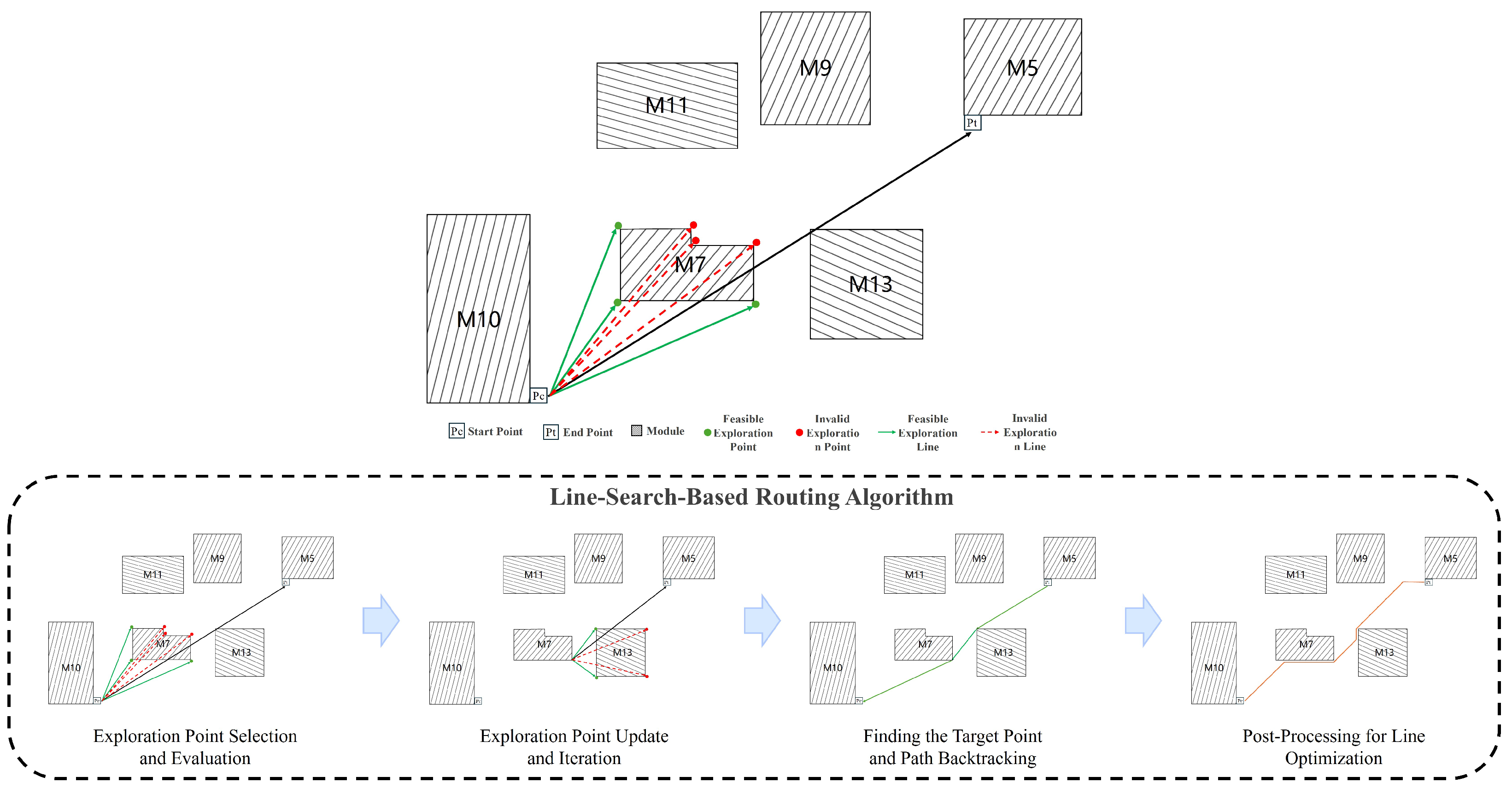
Our routing process consists of four steps: exploration point selection and evaluation, exploration point update and iteration, finding the endpoint/path backtracking, and post-processing of the line type. The routing process is illustrated in Figure 4. To complete the routing of a placement using the line-search algorithm, we first determine the start and end points of the connections based on the given netlist data and then use the line-search algorithm to connect the start and end points.

In the integrated circuit (IC) routing process, the nets in the netlist can be divided into two-terminal nets and multi-terminal nets. For two-terminal nets, since their connection relationships are clear, the pins of the two endpoints can be directly used as the start and end points for routing.

For multi-terminal nets, the connection relationships are not yet determined. To minimize the total wirelength, we employ the Minimum Spanning Tree (MST) algorithm to determine the connection relationships between the endpoints. The MST algorithm ensures a tree-structured network where the total weight of the edges (the distance between pins) is minimized. Let the set of endpoints for a multi-terminal net be $P=\{P_1,P_2,\cdots ,P_n\}$, where n is the number of endpoints. The goal of the MST algorithm is to find a tree connecting all endpoints such that the total weight of the edges (the distance between pins) is minimized. We use Kruskal’s algorithm, which sorts all edges in ascending order of weight and adds them to the tree one by one, ensuring no cycles are formed, until the tree includes all endpoints.

To ensure that the connection points are located outside the module where the pin resides, an out-routing strategy is applied to the pins as follows (Figure 5):

• Module Expansion: Expand the module by a distance equal to the module’s space plus half the wire width, resulting in expandModule. The out-routing points must lie on or outside its boundary.
• Calculate Minimum Distance: Calculate the minimum distance $minDis$ from each side of the pin to expandModule.
• Select Feasible Edges: Select edges whose distance to expandModule is less than $k·minDis$ as feasible edges, where $k\ge 2$.
• Determine Feasible Out-Routing Points: Compute the projection points from the pin’s center to the feasible edges, obtaining the feasible out-routing point set $P_{feasible}$.
• Filter Conflicts: Filter out points located inside obstacles or where the out-routing segment is blocked, resulting in $P_{feasible}^{\prime }$.
• Select Optimal Point: Choose the point with the shortest distance to the target point as the optimal out-routing point $P_{optimal}$:

  $$P_{optimal}=arg\underset{P_i\in P_{feasible}^{\prime }}{min}d(P_i,P_{target})$$

  (11)
• Candidate Out-Routing Points: Add the points in $P_{feasible}^{\prime }$ (excluding the optimal out-routing point) as candidate points to the openlist.

4.4.1. Routing Process

The line-search-based routing algorithm aims to solve the path planning problem from the start pin ($P_c$) to the target pin ($P_t$). By selecting exploration points and evaluating their costs, the algorithm gradually approaches and ultimately determines the shortest path.

Algorithm Initialization

First, define the start and target points. The start point $P_c$ is the beginning of the routing, typically the optimal out-routing point of a pin. The target point $P_t$ is the destination of the routing, usually the optimal out-routing point of another pin or a point on an already routed segment.

Next, initialize the open list by adding the feasible out-routing points of the start point. The open list is used to store points to be explored. Simultaneously, initialize the closed list as an empty set, which records the points that have already been explored.

Finally, define the cost function $f\left(n\right)$, expressed as

$$f\left(n\right)=g\left(n\right)+h\left(n\right)$$

(12)

where $g\left(n\right)$ represents the cumulative path cost from the start point $P_c$ to the current exploration point n, and $h\left(n\right)$ represents the heuristic estimated cost from the current exploration point n to the target point $P_t$:

$$h\left(n\right)=|n_x-P_{t_x}|+|n_y-P_{t_y}|$$

(13)

Exploration Point Selection and Evaluation

From the current exploration point $P_c$, a ray is projected toward the target point $P_t$ until it encounters the first obstacle. The endpoints of the first obstacle are considered to be potential exploration points.

For each obstacle endpoint $P_e$, check whether the line connecting the current exploration point $P_c$ to the endpoint $P_e$ intersects with the obstacle. If the line passes through the obstacle, the endpoint is excluded. If the line does not pass through this obstacle but intersects with other obstacles, the endpoints of the new obstacles are added to the feasibility check. If the line does not intersect any obstacles, the endpoint $P_e$ is considered to be a feasible exploration point.

All feasible exploration points are added to the open list, and their cost $f\left(P_e\right)$ and parent node (the current point $P_c$) are recorded.

Exploration Point Update and Iteration

Sort the points in the open list based on their cost $f\left(n\right)$, and select the point with the minimum cost as the next exploration point. This is typically implemented using a min-heap or priority queue for fast access to the point with the lowest cost.

Select the point with the minimum cost $P_{best}$, remove it from the open list, and add it to the closed list. Set $P_{best}$ as the new current exploration point, and repeat the exploration point selection and evaluation steps to continue searching toward the target point.

Finding the Target Point and Path Backtracking

When an exploration point coincides with or is sufficiently close to the target point $P_t$, it indicates that a path from the start point $P_c$ to the target point $P_t$ has been found, and the exploration process is terminated.

Construct the complete path by backtracking through the parent node information of each exploration point. Starting from the target point $P_t$, use the parent node information of each exploration point to trace back to the start point $P_c$. The sequence of nodes formed during backtracking represents the shortest path from the target point to the start point. Finally, reverse the path sequence to obtain the final path from the start point $P_c$ to the target point $P_t$.

Post-Processing for Line Optimization

To meet routing constraints, post-processing optimization is performed on the computed path to eliminate unnecessary detours and satisfy angle constraints.

First, check whether the path can be simplified by directly connecting segments. If a segment of the path can be directly connected to a subsequent point without intersecting obstacles, perform the direct connection.

Next, decompose all successful direct connections into vectors. A diagonal line can be decomposed into a straight segment followed by a 135-degree segment, thereby satisfying angle constraints in the overall routing. The optimization process is illustrated in Figure 6.

5. Experiments

5.1. Experimental Environment

The experiments in this paper were conducted using the Python 3.11 programming language and the Scikit-learn machine learning library. The experimental platform was an HP laptop with an Intel(R) Core(TM) i5-13500HX processor running at 2.50 GHz and 16.0 GB of RAM.

5.2. Dataset

In this experiment, we used Analog IC data provided by Empyrean, including 200 cases. The dataset contains diverse Analog IC placement and routing cases with varying initial placement results. The differences between these placements include the placement area (i.e., layout dimensions) as well as the shapes and sizes of the modules. Each module is equipped with 3 pins.

5.3. Experimental Metrics

5.3.1. Metrics for Placement Optimization

In Analog IC layout design, the following key metrics are used to evaluate the performance of the placement algorithm:

Routing Connectivity Ratio: The ratio of successfully routed connections to the total number of connections. RCR reflects the algorithm’s ability to solve routing problems and is an important metric for assessing the feasibility and effectiveness of the algorithm.

Wirelength: The total length of all routed nets. Shorter wirelength implies higher signal transmission efficiency, lower signal delay, and reduced energy loss.

Runtime: The total time required to optimize the placement. Shorter runtime indicates higher algorithm efficiency.

5.3.2. Metrics for Routability Prediction Model

To evaluate the performance of the random-forest-based routability prediction model, the experiment collected and constructed a dataset by adjusting each placement in the dataset 400 times. The dataset was split into training and testing sets in an 8:2 ratio. The model’s performance was evaluated using metrics such as accuracy, precision, F1 score, and recall. The definitions of the variables used in these metrics are summarized in

Table 1. Variable definitions.

Variable	Definition
TP	Number of placements where both predicted and true values are good layouts
TN	Number of placements where both predicted and true values are not good layouts
FP	Number of placements where the predicted value is a good layout but the true value is not
FN	Number of placements where the true value is a good layout but the predicted value is not

.

5.4. Experimental Results

5.4.1. Performance Evaluation of Placement Optimization Algorithms

To validate the effectiveness of the proposed placement and routing co-optimization framework and compare the performance of different optimization algorithms under this framework, we selected four representative placement optimization algorithms for experimentation: parallel particle swarm optimization [9], simulated annealing, IBE-SMO [10], and reinforcement learning [13]. Additionally, we compared the performance of these algorithms when using HPWL as the direct optimization objective. In our placement optimization, the algorithm was set to perform 20 rounds of optimization, with 7 adjustments per round. To ensure fairness and consistency, we configured reasonable parameters for each algorithm and conducted experiments under the same number of optimization iterations. To further verify the effectiveness of the optimization algorithm used in this paper, we compared the algorithms under the placement and routing co-optimization framework with those using HPWL as the optimization objective. The specific results show the average routing connectivity ratio, average total wirelength, and average HPWL for all cases in the dataset.

Table 2. Performance comparison of different algorithms.

Category	Algorithm	RCR	Wirelength	HPWL	Overlap	Spacing	DRC
Co-Optimization	PA (0.75)	0.915	5969.481	5117.135	0	100%	0
	PA (0.8)	0.912	6302.830	5257.120	0	100%	0
	PA (0.85)	0.915	6232.728	5239.985	0	100%	0
	Reinforcement Learning [13]	0.903	6221.394	5304.307	0	100%	0
	IBE-SMO [10]	0.911	6163.019	5300.555	0	100%	0
	Parallel PSO [9]	0.895	6744.612	5547.520	0	100%	0
	Simulated Annealing	0.897	6750.029	5577.180	0	100%	0
HPWL-Based	Reinforcement Learning-HPWL [13]	0.792	5280.701	4246.639	0	100%	0
	IBE-SMO-HPWL [10]	0.798	5205.646	4035.354	0	100%	0
	Parallel PSO-HPWL [9]	0.786	5715.939	4772.744	0	100%	0
	Simulated Annealing-HPWL	0.798	5163.845	3993.460	0	100%	0

PA: The proposed algorithm.

compares the performance of various optimization algorithms under two optimization objectives: one using the placement and routing co-optimization framework and the other using HPWL as the sole optimization objective. From the data in the table, it can be observed that the algorithms under the placement and routing co-optimization framework significantly outperform the HPWL-based methods in terms of routing connectivity ratio (RCR). Under the co-optimization framework, the proposed algorithm and other optimization methods maintain RCRs between 0.895 and 0.915, while the HPWL-based methods achieve RCRs of only 0.792 to 0.798. Compared to the HPWL-based methods, the four algorithms using the co-optimization framework improve RCR by 12.41%, 14.16%, 13.87%, and 14.02%, respectively. Although the HPWL-based methods perform better in terms of total wirelength and HPWL, their lower RCRs indicate that some signal lines may fail to route due to limited placement or routing resources, potentially leading to functional failures in the design. RCR is a critical metric for evaluating placement quality, directly impacting the realizability of the design. In summary, although the co-optimization method may slightly sacrifice total wirelength, it significantly improves the routability and functional integrity of the design.

To further validate the effectiveness of the optimization algorithm employed in this study, we have provided a detailed presentation of selected cases from the dataset. The specific results show the routing connectivity ratio (RCR) and wirelength for each case. Additionally, to better evaluate the algorithm’s performance on the entire dataset, we also recorded the results of layout optimization using routability prediction models trained with different thresholds.

Table 3. Comparison of routing connectivity ratio and wirelength.

Case ID	Initial Placement		PA (0.75)		PA (0.8)		PA (0.85)		RL [13]		IBE-SMO [10]		Parallel PSO [9]		SA
	RCR	WL	RCR	WL	RCR	WL	RCR	WL	RCR	WL	RCR	WL	RCR	WL	RCR	WL
10001	0.941	5206.971	0.882	4879.091	0.941	6403.517	0.941	6062.813	0.941	5028.085	0.882	6080.49	0.941	8138.678	0.882	6038.434
10002	0.882	6293.445	0.941	4000.315	0.941	5418.64	0.882	3809.978	0.882	5776.723	0.882	3699.176	0.882	5930.207	0.882	4440.698
10004	0.765	6075.277	0.941	5179.995	0.941	5930.745	0.882	4510.318	0.941	6471.043	0.941	3987.02	0.941	5595.654	0.941	6760.673
10005	0.882	6172.21	0.941	3237.318	0.941	5065.73	0.941	3915.699	0.882	4435.12	0.941	3583.397	0.882	4208.416	0.882	4631.874
10006	0.882	5674.33	0.941	3958.555	0.882	5025.012	0.941	4849.779	0.941	4805.545	0.941	4767.605	0.882	5776.663	0.882	4943.004
10008	0.941	6547.302	0.941	5155.317	0.941	4253.622	0.941	4180.55	0.941	6149.592	0.941	4724.613	0.941	4572.816	0.941	6703.389
10009	0.824	5957.245	0.941	3740.63	0.941	3484.836	0.941	3982.944	0.941	4073.259	0.882	3796.117	0.882	4707.662	0.941	4986.1
10010	0.941	4546.271	0.941	4463.599	0.941	5231.784	0.941	6279.741	0.941	3969.503	0.882	4685.925	0.941	4528.776	0.941	4429.023
10011	0.824	6451.533	0.941	4683.128	0.941	4734.158	0.941	4281.114	0.941	5063.857	0.882	4221.644	0.941	4739.037	0.941	4215.544
10012	0.941	3580.156	0.941	5256.315	0.882	5694.23	0.941	6814.285	0.882	6150.21	0.941	4689.049	0.882	4753.011	0.941	5082.377
…	…	…	…	…	…	…	…	…	…	…	…	…	…	…	…	…
10030	0.824	6911.526	0.882	6219.029	0.941	4595.954	0.941	5489.794	0.941	5635.468	0.941	4268.517	0.941	5116.385	0.882	5909.298
10031	0.941	6107.221	0.941	3599.062	0.941	4699.963	0.941	6292.646	0.941	5930.948	0.882	4992.588	0.882	5238.03	0.941	6361.102
10032	0.882	6379.322	0.941	4287.723	0.882	4726.846	0.941	5668.645	0.941	6312.388	0.941	4731.601	0.882	5611.361	0.941	6837.782
10033	0.882	6096.661	0.941	5662.346	0.882	4538.144	0.941	5194.275	0.941	4874.624	0.941	4634.462	0.941	4944.741	0.941	5355.09
10050	0.882	4890.467	0.941	5741.959	0.941	5574.509	0.941	5025.478	0.882	4755.527	0.941	4684.835	0.941	3853.909	0.941	4835.154
10091	0.75	7842.595	0.917	7529.396	0.917	7104.183	0.917	7670.842	0.917	8068.445	0.917	8670.959	0.917	6322.479	0.875	8801.311
10092	0.75	11,110.156	0.833	6499.66	0.875	8178.585	0.833	7096.52	0.833	7975.611	0.875	9124.681	0.875	11,281.018	0.875	11,567.161
10093	0.875	11,328.563	0.875	6393.204	0.917	8526.584	0.917	8344.377	0.917	8378.664	0.958	7881.006	0.917	8571.532	0.917	8557.43
10095	0.833	8495.816	0.958	7120.832	0.958	8679.724	0.958	8109.369	0.958	9767.678	0.958	5863.245	0.917	8104.383	0.958	7836.414
10096	0.917	8202.314	0.958	9355.469	1.0	10,627.672	1.0	10,630.485	0.917	8959.312	0.875	9747.764	0.917	10,671.226	0.958	8122.323
…	…	…	…	…	…	…	…	…	…	…	…	…	…	…	…	…
10163	0.875	11,545.602	0.917	9118.632	0.917	9459.82	0.917	7789.148	0.875	6894.495	0.958	7827.072	0.917	8348.056	0.958	11,654.583
10165	0.833	12,110.143	0.917	9415.3	0.875	11,364.135	0.875	8505.267	0.875	10,741.739	0.958	12,189.316	0.917	10,596.339	0.958	10,292.953
10167	0.833	11,062.7	0.917	7572.878	0.958	7329.915	0.917	7446.907	0.917	7736.204	0.917	8096.176	0.917	9713.699	0.917	10,863.554
10168	0.833	13,115.742	0.958	9320.479	0.958	8776.489	0.917	7930.812	0.958	9424.878	0.917	6340.694	0.917	10,536.999	0.917	8285.565
10169	0.917	13,980.591	0.917	7208.464	0.958	8039.805	0.917	10,460.622	0.833	9259.954	0.917	9288.404	0.917	8905.053	0.875	9439.341
10172	0.833	10,554.676	0.917	7520.045	0.958	8003.571	0.958	9379.509	0.958	8976.284	0.958	12,015.409	0.917	10,861.896	0.917	8975.129
10173	0.667	9887.088	0.833	7228.779	0.875	8619.162	0.875	7827.829	0.792	8279.56	0.875	8691.527	0.833	8308.236	0.833	8142.874
10174	0.833	7805.881	0.875	7625.748	0.833	9905.66	0.875	10,002.228	0.833	6139.362	0.875	9701.708	0.875	9264.415	0.833	6976.59
10175	0.708	7708.52	0.833	8657.922	0.875	8528.689	0.875	6252.564	0.875	4834.054	0.792	7488.855	0.792	8652.546	0.833	7862.552
10176	0.833	10,206.05	1.0	10,548.643	0.917	8939.841	0.917	7504.896	1.0	9312.48	0.917	9062.072	0.917	10,069.069	0.958	9717.85
…	…	…	…	…	…	…	…	…	…	…	…	…	…	…	…	…
Average	0.847	7309.667	0.915	5969.481	0.912	6302.830	0.915	6232.728	0.903	6221.394	0.911	6163.019	0.895	6744.612	0.897	6750.029

PA: The proposed algorithm.

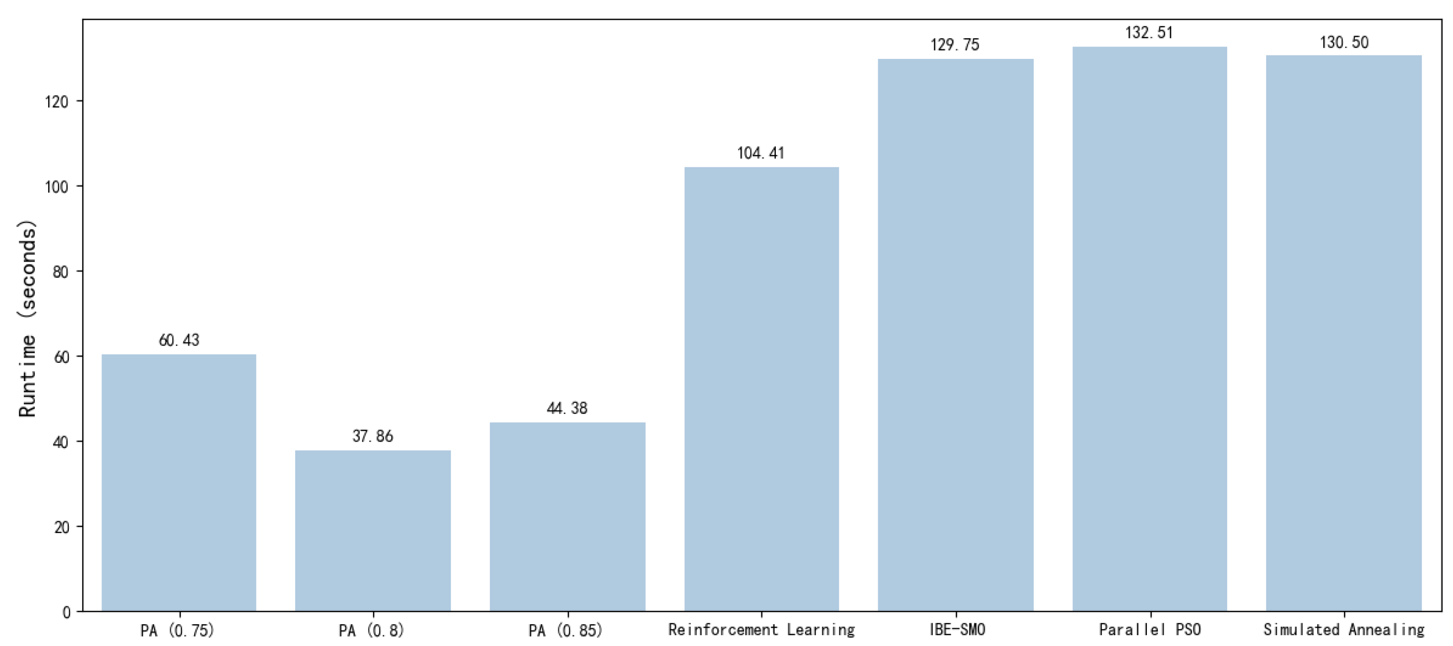
lists the RCR and wirelength data after optimization using different algorithms on the datasets. Figure 7 shows the average time required for optimization by each algorithm.

From Table 3 and Figure 7, it can be observed that, when the proposed algorithm uses a routability prediction model with a threshold of 0.75 for layout optimization, it outperforms the other four algorithms in terms of average RCR and average wirelength on the dataset. The proposed algorithm achieves an average RCR of 0.915 and an average wirelength of 5969.481, representing an 8.03% improvement in RCR compared to the initial layout’s average RCR of 0.847 and an 18.33% reduction in wirelength compared to the initial layout’s average wirelength of 7309.667. Among the other comparison algorithms, IBE-SMO performs the best, with an average RCR of 0.911 and an average wirelength of 6163.019, but it still falls short of the proposed algorithm’s results.

In terms of time efficiency, when using a routability prediction model with a threshold of 0.8 for layout optimization, the proposed algorithm completes the layout optimization for 200 test cases in an average of 37.86 s, which is 63.8% faster than reinforcement learning (104.41 s), the fastest among the four comparison algorithms. Even when using a routability prediction model with a threshold of 0.75, the proposed algorithm takes an average of 60.43 s, which is still better than the other four algorithms.

In summary, the proposed algorithm demonstrates outstanding performance in RCR, wirelength, and time efficiency when using a routability prediction model with a threshold of 0.75 for layout optimization, significantly outperforming the other four algorithms.

5.4.2. Comparison of Routability Prediction Performance

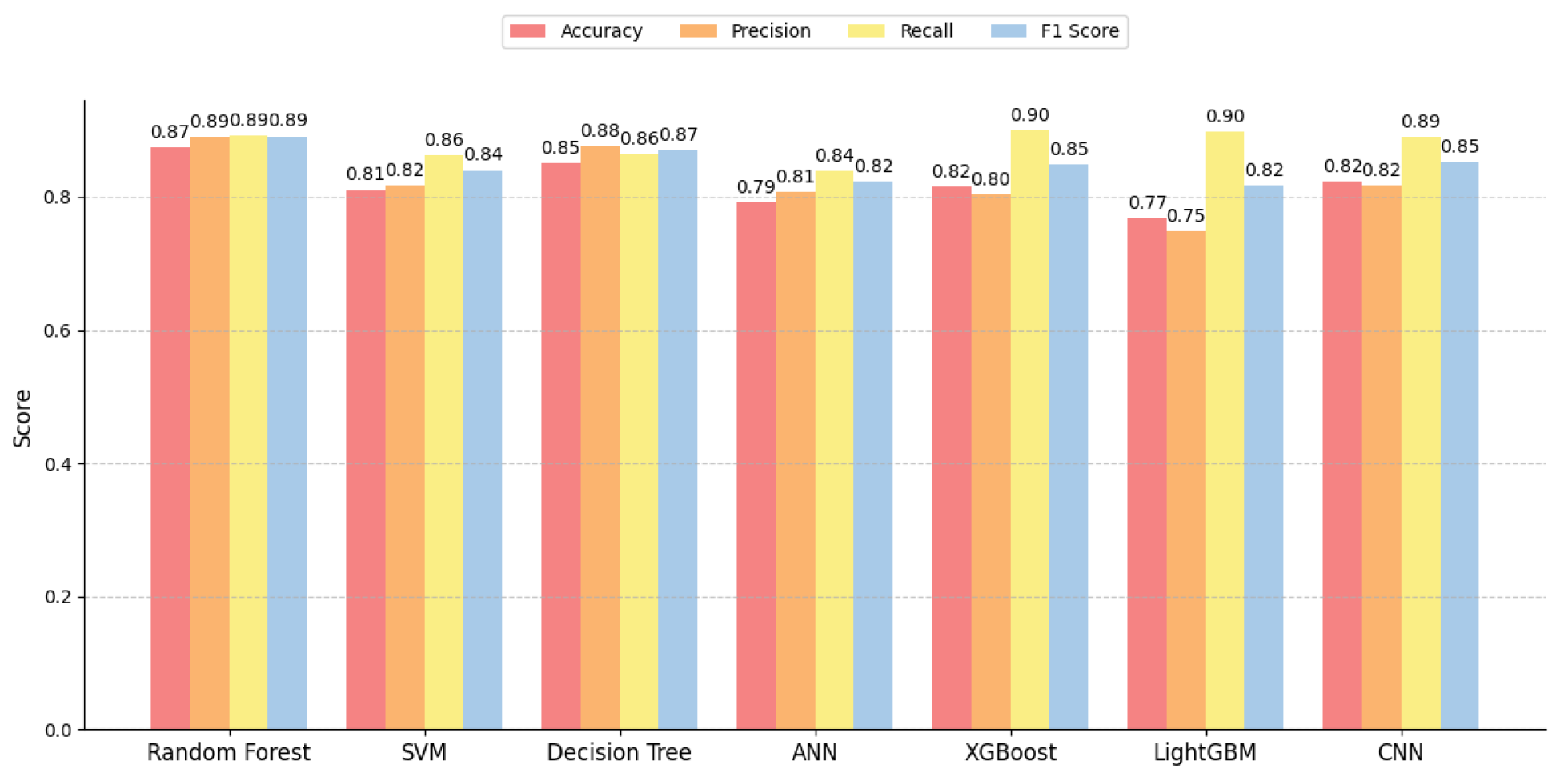
To evaluate the performance of the routability prediction model, this study employs the random forest algorithm [20] as the baseline model and compares it with other commonly used machine learning algorithms, including SVM [21], decision trees [22], ANN [23], XGBoost [24], LightGBM [25], and CNN [26]. For different classification threshold strategies, we evaluate the performance of each model on the same dataset using metrics such as accuracy, precision, recall, and F1 score. Figure 8, Figure 9 and Figure 10 show the comparison of prediction performance among different models at different thresholds. At the same time, we also compared the time required for each model to predict a single layout with the time required for routing a single layout, as shown in

Table 4. Comparison of prediction times for different models and wiring algorithm routing time.

Algorithm	Time (s)
Wiring Algorithm	0.7571
Random Forest	0.002
Support Vector Machine	0.0422
Decision Tree	0.0002
Artificial Neural Network	0.0002
XGBoost	0.0009
LightGBM	0.001
CNN	0.0013

.

By comparing the results, it can be concluded that random forest performed relatively well in this experiment. Especially when handling complex, high-dimensional data, it demonstrated strong generalization capabilities. Not only did it show a significant advantage in prediction accuracy but its prediction time efficiency was also relatively ideal. Therefore, we chose random forest as the model for routability prediction.

5.4.3. Threshold Analysis

The primary function of the routability prediction model is to filter out layouts with poor routing connectivity ratios, thereby enhancing the efficiency and quality of layout optimization. In selecting the model threshold, we tested three distinct thresholds (0.75, 0.8, and 0.85), applying each to our layout algorithms. The following are the analysis results:

When trained with a threshold of 0.75, the routability prediction model combined with the optimization algorithm achieved the highest routing connectivity ratio (0.915) and the lowest wirelength (5969.481). Given the lower threshold, fewer layouts were filtered by the model, allowing the optimization process to focus on improving wirelength when the routing connectivity ratio was equal. This led to optimal wirelength performance but also increased computational time. Overall, the model with a threshold of 0.75 achieved a good balance between routing connectivity ratio and wirelength.

At a threshold of 0.8, as the threshold increased, the model discarded more potentially viable layouts, resulting in a significant drop in recall, indicating reduced capability in identifying better layouts. While this stricter filtering strategy decreased optimization time, it also overlooked some moderately high-quality layouts, leading to suboptimal performance in both routing connectivity ratio and wirelength. Therefore, the model at a threshold of 0.8 showed poorer balance between quality and efficiency.

With a threshold of 0.85, further increasing the threshold made the model’s filtering approach even more stringent, leading to declines in both precision and recall, signifying further diminished ability to identify better layouts. This strategy prioritized the enhancement of the routing connectivity ratio over wirelength optimization. However, due to the probabilistic routing mechanism embedded in the layout algorithm, layouts that did not meet the 0.85 routing connectivity ratio might still be routed, maintaining the routing connectivity ratio at 0.915, with slightly longer computational times compared to the threshold of 0.8.

Considering the overall performance in terms of routing connectivity ratio, wirelength, and computational time, the routability prediction model with a threshold of 0.75 performed optimally for the current task, achieving a superior balance between layout quality and optimization efficiency. The routability prediction model trained at this threshold, together with the layout optimization algorithm, significantly improved the performance of routing connectivity ratio and wirelength while reducing optimization time through an effective filtering strategy of low-quality layouts.

5.4.4. Case Study Analysis

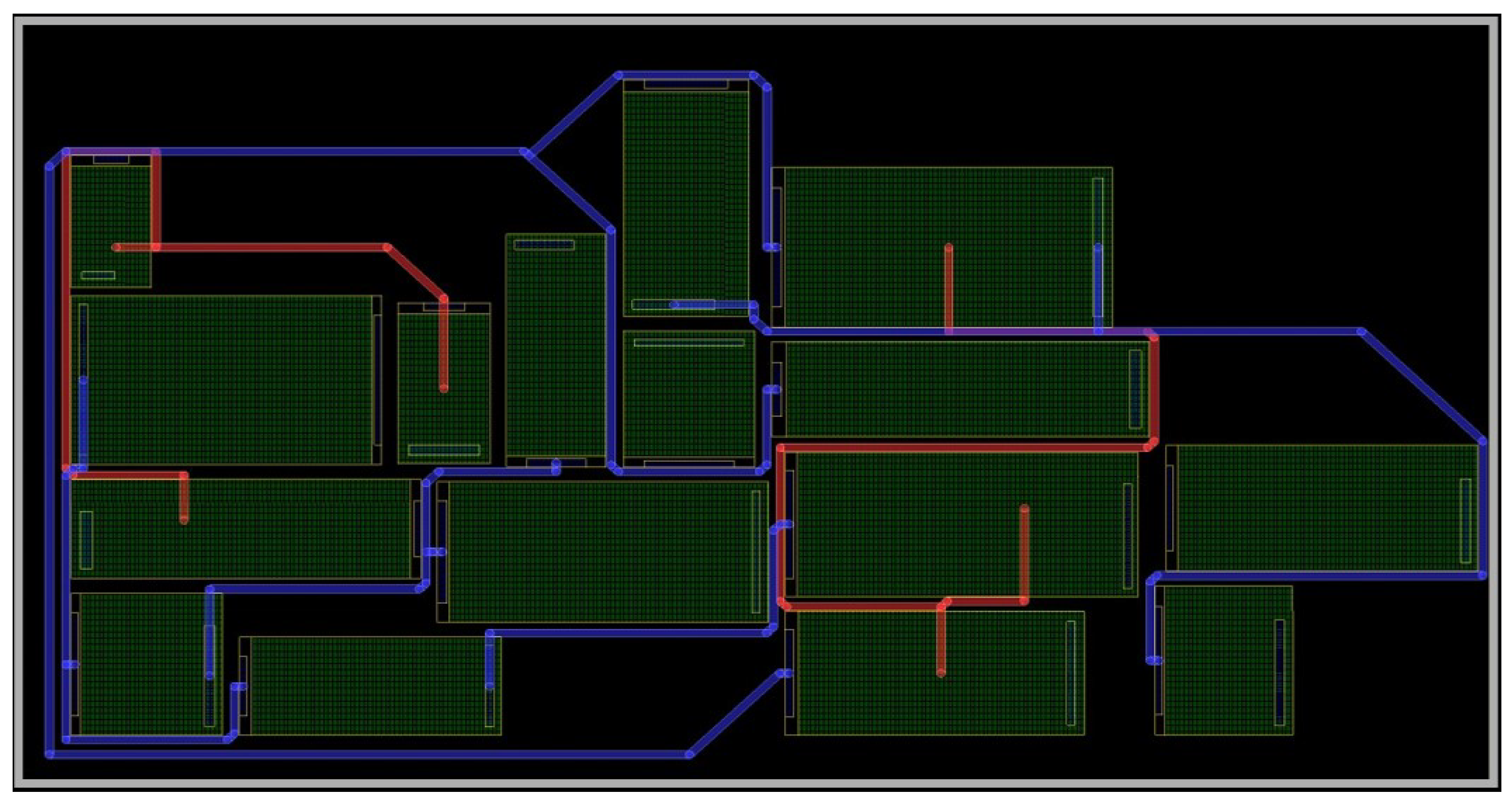
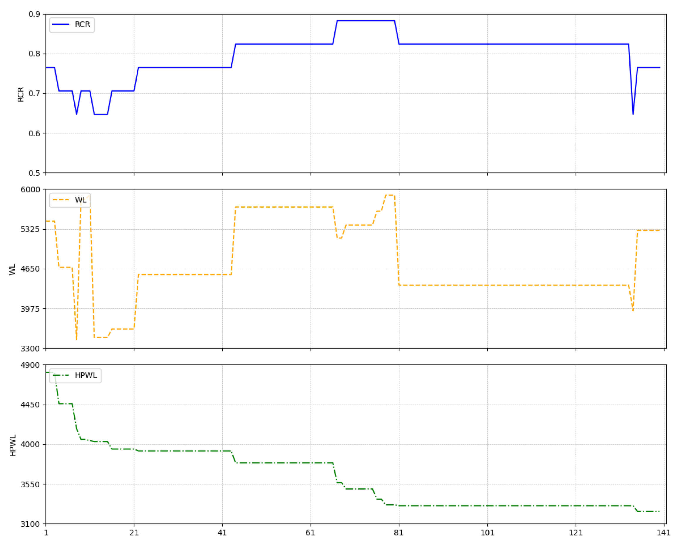
Figure 11 shows the routing result of the initial layout for case 10054, where red and blue lines represent different routing layers. The achieved routing connectivity ratio is 0.706, with a wirelength of 6239.297. Figure 12 presents the result of placement and routing optimization using the simulated annealing algorithm with HPWL as the optimization objective. After 140 adjustments, the routing connectivity ratio increased to 0.765, and the wirelength was reduced to 5300.374. 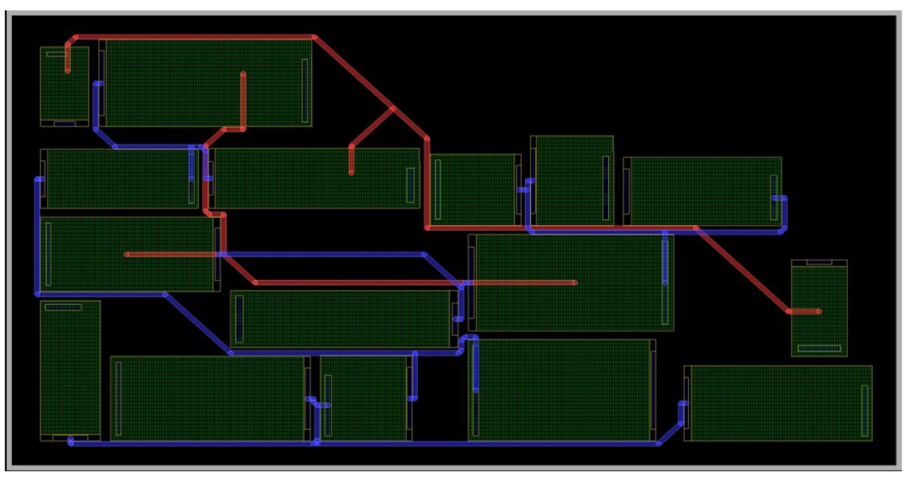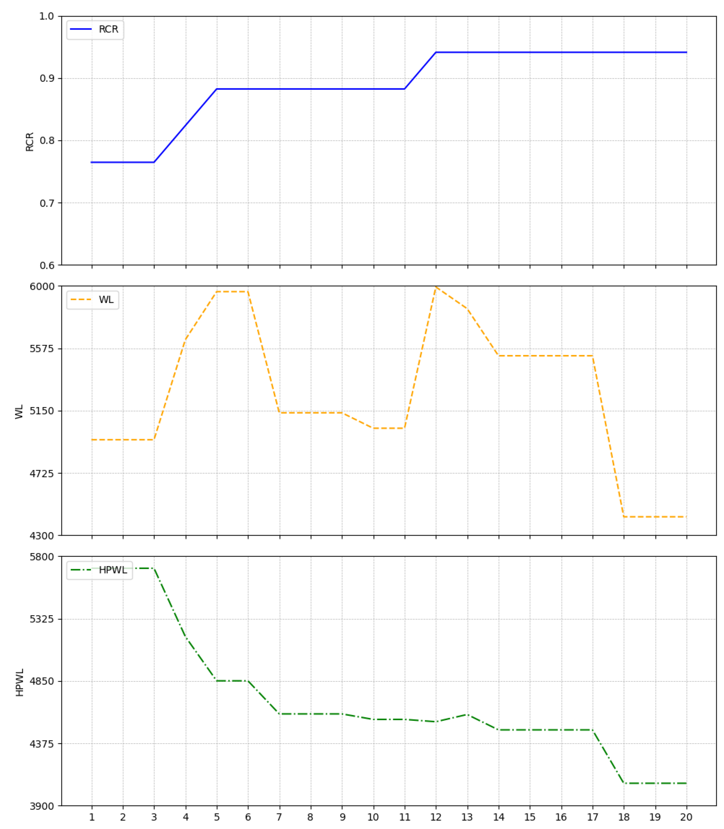Figure 13 displays the optimized layout achieved by the proposed algorithm, with 20 rounds of optimization, each consisting of 7 adjustments. The routing connectivity ratio improved to 0.941, and the wirelength was shortened to 4426.264. Figure 14 illustrates the optimization process using the simulated annealing algorithm based on HPWL as the optimization objective, while Figure 15 shows the optimization process of the proposed algorithm.

The improvements in both routing connectivity ratio and wirelength indicate that the proposed algorithm has effectively enhanced the interconnect efficiency between modules, minimized the potential for signal conflicts, and improved spatial utilization and overall performance of the IC layout by shortening the wirelength. The layout resulting from optimization for HPWL is notably compact due to its focus on minimizing HPWL without considering routing constraints, leading to congestion and detours in wiring paths. This comparison underscores the effectiveness of the proposed algorithm in addressing layout optimization challenges.

6. Future Work

The placement and routing co-optimization method proposed in this paper, although providing an innovative optimization approach in the field of integrated circuit design and achieving significant results, still has many aspects that can be expanded upon and improved based on the current research foundation and experimental results.

Firstly, the current research primarily considers boundary constraints and non-overlap constraints. Future work could explore how to incorporate other complex constraints that are commonly encountered in practical integrated circuit design into the placement and routing co-optimization framework. This would further enhance the overall performance of the design.

In terms of the routability prediction model, this paper employs the random forest algorithm as the core method. However, given the significant advancements in deep learning techniques for placement and routing optimization in recent years, integrating deep learning technologies into the co-optimization process holds the potential to further improve optimization outcomes and enhance the predictive capability of the model.

Additionally, the scale of the experimental dataset used in this study is relatively small, which limits the generalization ability and robustness verification of the algorithm. To significantly enhance its placement capabilities and generalization performance, it is necessary to conduct training on a more diverse set of circuit modules. This not only imposes higher requirements on the scale of the dataset but also presents new challenges in terms of the richness and diversity of the circuit modules. Expanding the dataset to include more complex scenarios will provide more comprehensive validation of the effectiveness and adaptability of the proposed method.