
Towards Efficient Job Scheduling for Cumulative Data Processing in Multi-Cloud Environments

Abstract
1. Introduction
- (1)
- We propose the first comprehensive scheduling solution tailored for CDP applications.
- (2)
- We introduce the CDP-EM job execution model, supporting dynamic preprocessing job generation and automated, dependency-aware job execution.
- (3)
- We propose the PPO-based CDP-JS job scheduling strategy, capturing progress dynamics from job uncertainty and optimizing scheduling via historical learning.
- (4)
- We evaluate the proposed scheduling solution for CDP applications comprehensively using the real-world dataset and simulation experiments.
2. Related Works
2.1. Cloud Job Execution Model
2.2. Cloud Job Scheduling Strategy
3. Problem Definition
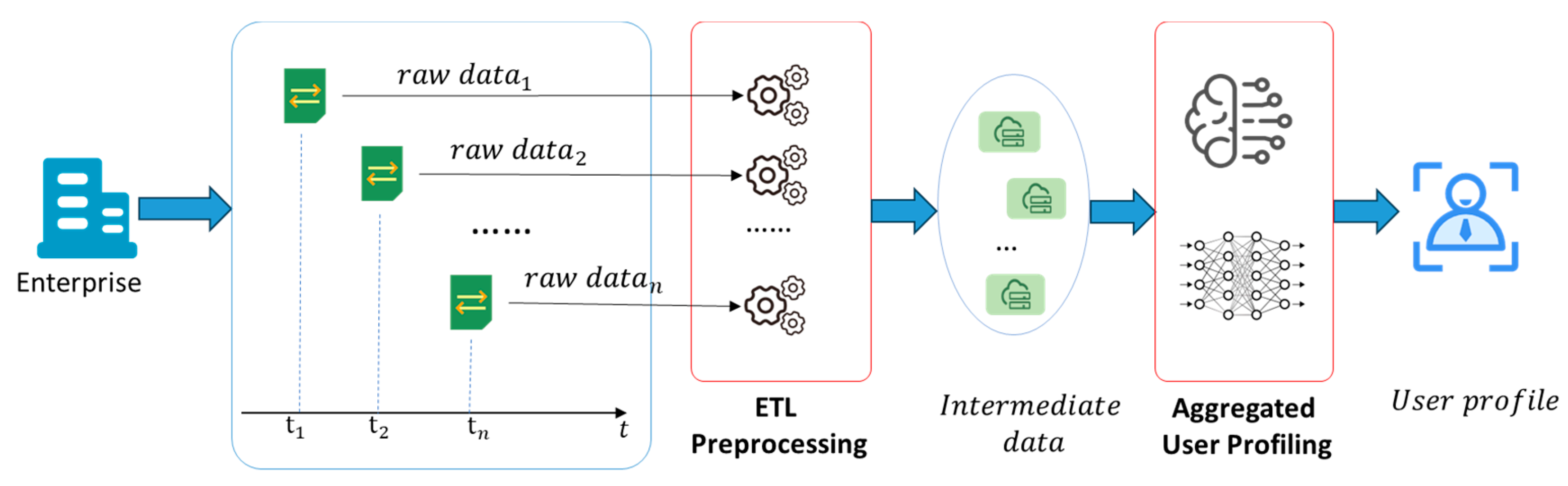
3.1. Cumulative Data Processing Application
3.2. Multi-Cloud Environment
3.3. Resource Cost
3.4. Problem Definition
4. Job Execution Model for CDP Applications
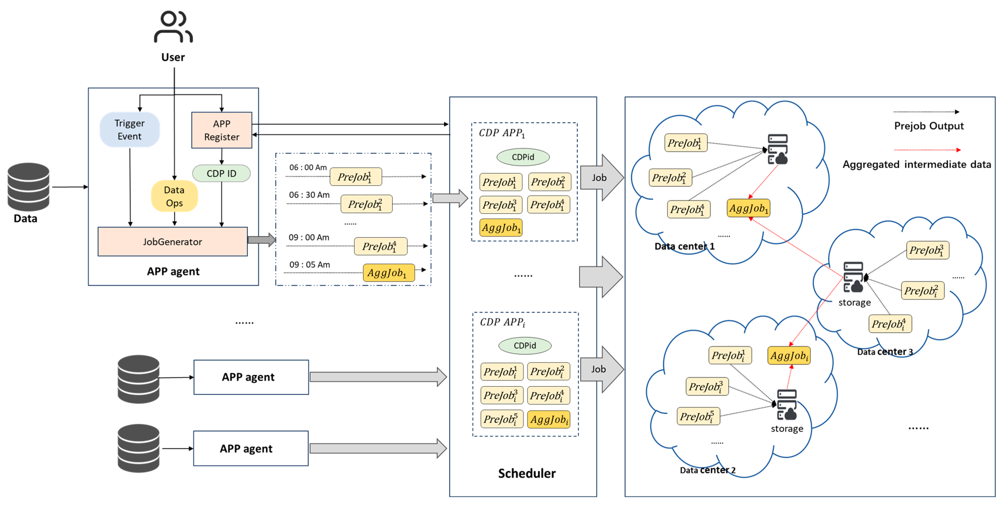
4.1. CDP-EM Model
4.2. Problem Redefinition
4.2.1. Calculation of
4.2.2. Calculation of
4.2.3. Calculation of
5. Job Scheduling Strategy for CDP Applications
5.1. Markov Decision Process Modeling
5.1.1. State Space
- Cloud Resource State
- 2.
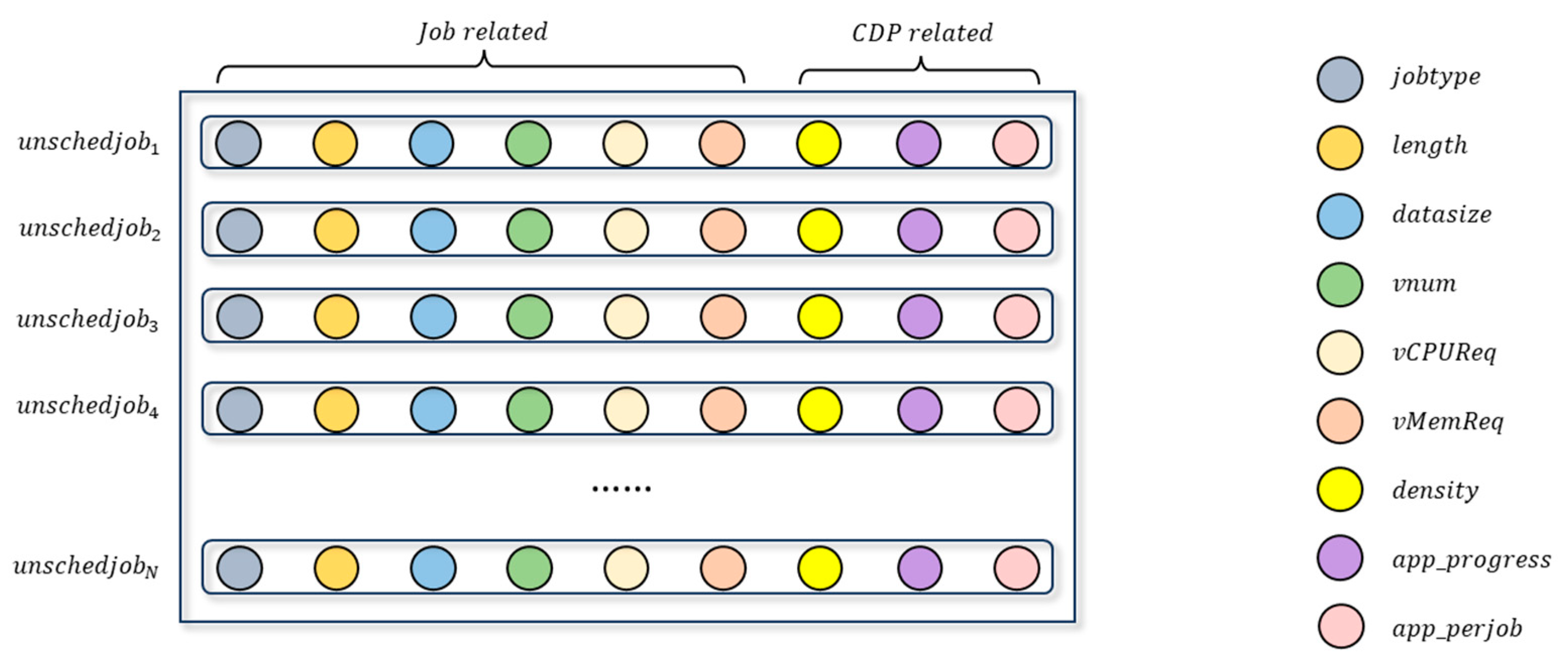
- Pending Job State
- 3.
- Historical Job Demand State
5.1.2. Action Space
5.1.3. Rewards
- Quality of VM Resource Allocation
- 2.
- Intermediate Data Distribution
- 3.
- Application SLA Violation Risk
- 4.
- Cost of Target Scheduled Job
- 5.
- Penalty for Unsuccessful Scheduling
5.2. PPO-Based Job Scheduling
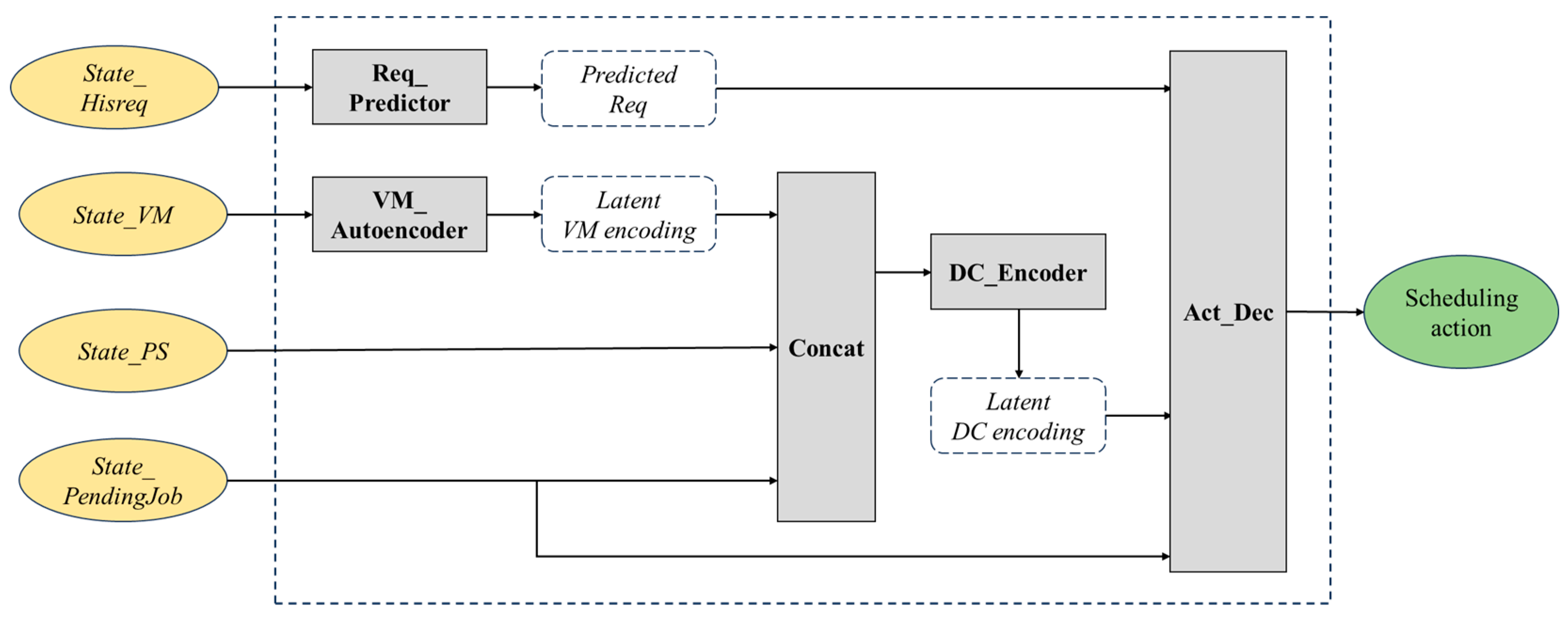
5.2.1. Actor and Critic Network Design
- VM_Autoencoder
- 2.
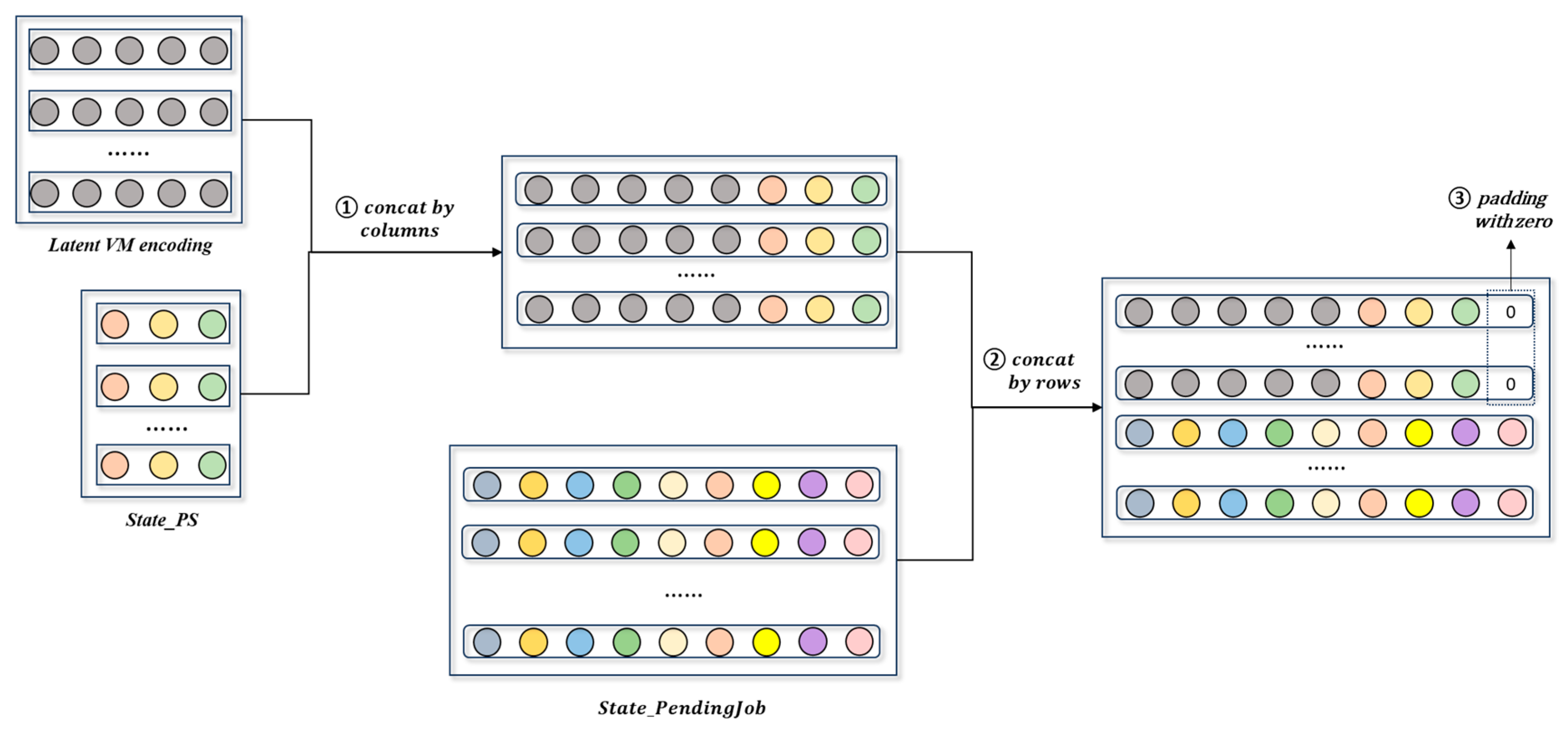
- Concat
- 3.
- DC_Encoder
- 4.
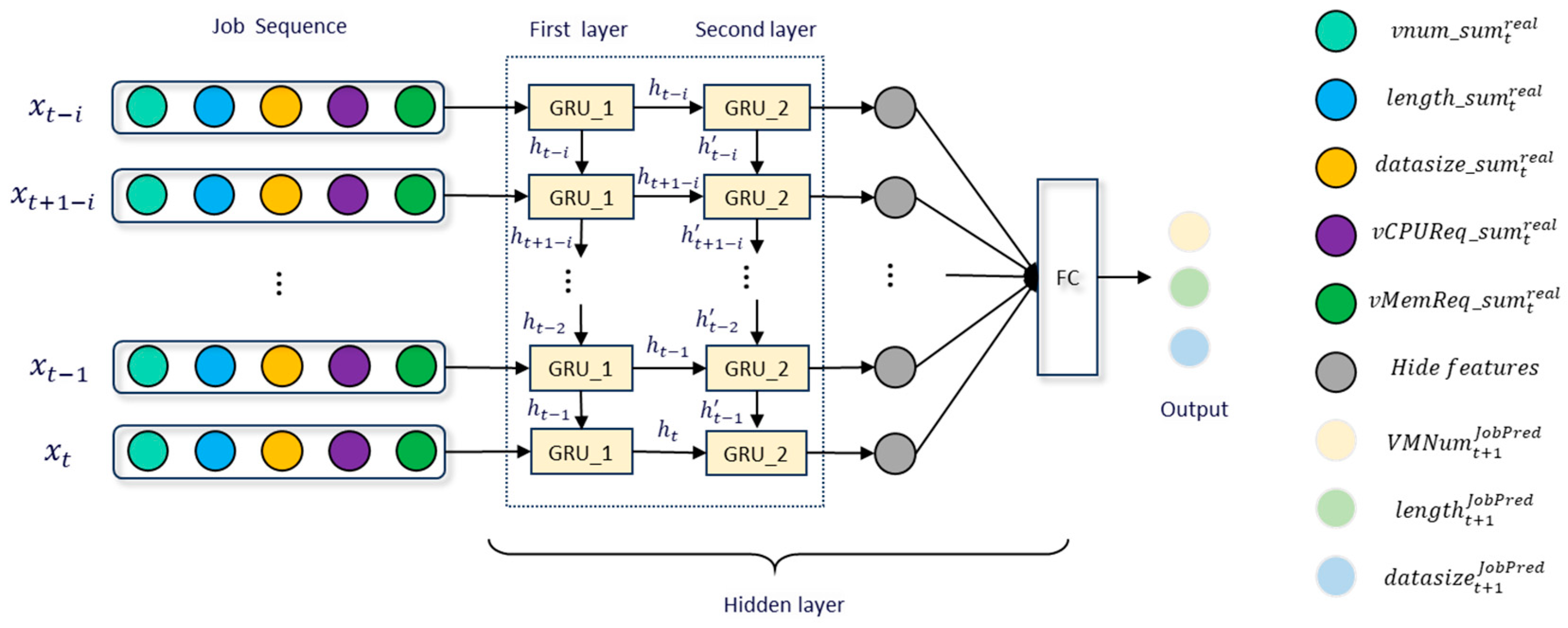
- Req_Predictor
- 5.
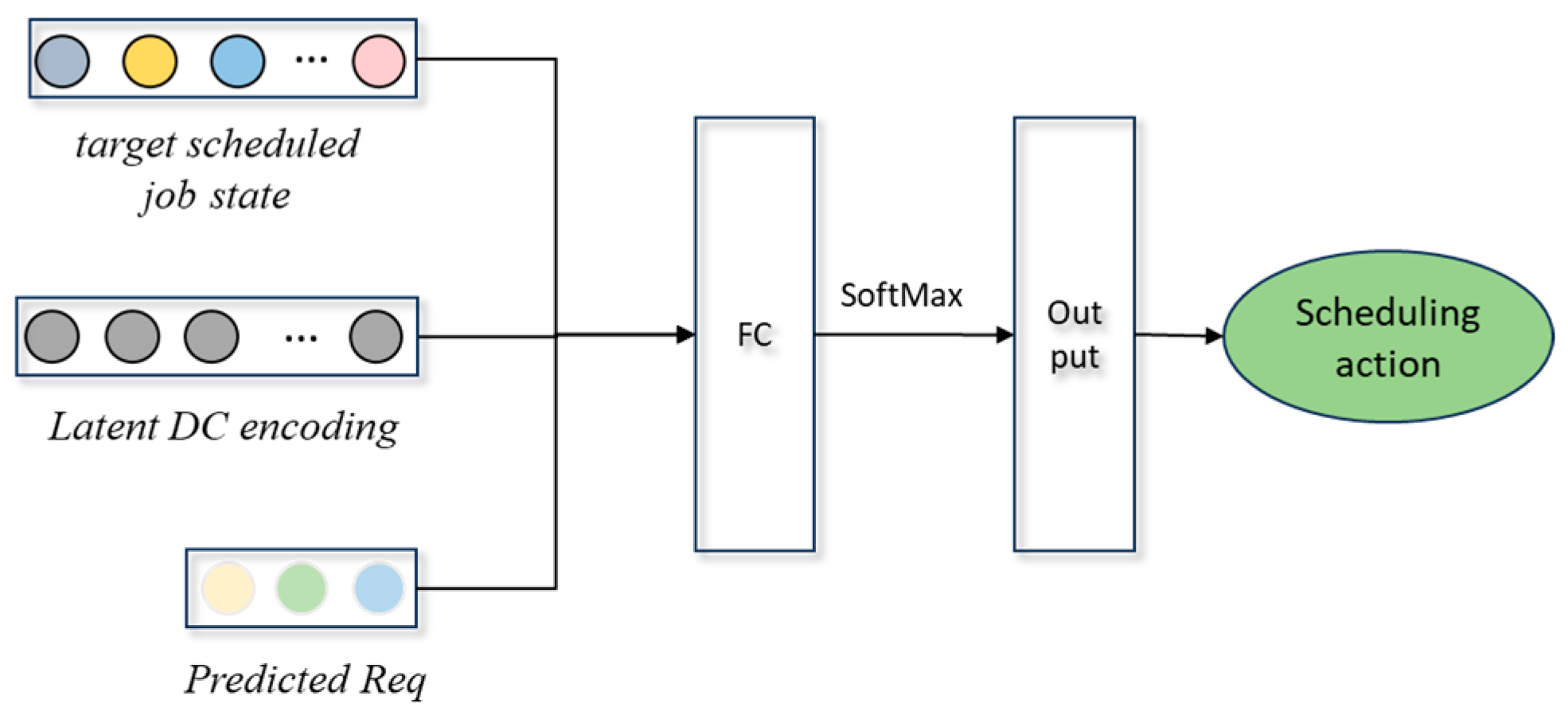
- Act_Dec
5.2.2. Training of Actor and Critic Network
6. Performance Evaluation
6.1. Experimental Settings
6.2. Performance Metrics
6.3. Baseline Methods
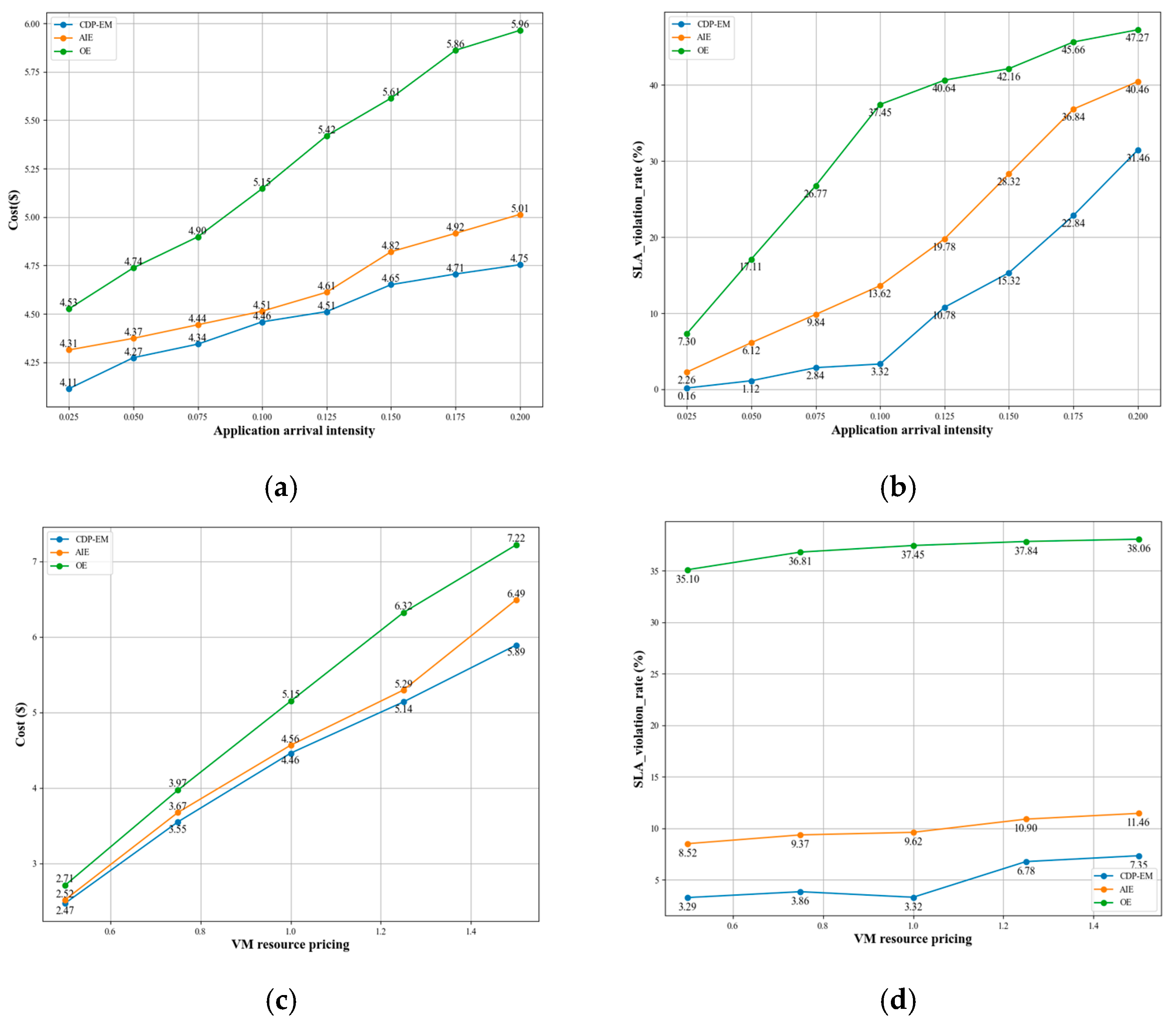
- One-off Execution (OE): Source data are continuously generated and accumulated until the acquisition deadline. Once reached, all the accumulated data are consolidated into a single job, which is then submitted to the cloud for preprocessing and aggregate analysis in one go.
- Anonymous Intermittent Execution (AIE): The accumulated source data are preprocessed in batches, with each batch corresponding to a preprocessing job. Once all preprocessing jobs are completed, the aggregate analysis job is submitted. All job submissions are manually triggered by the user and executed independently without reflecting any application ownership relationships.
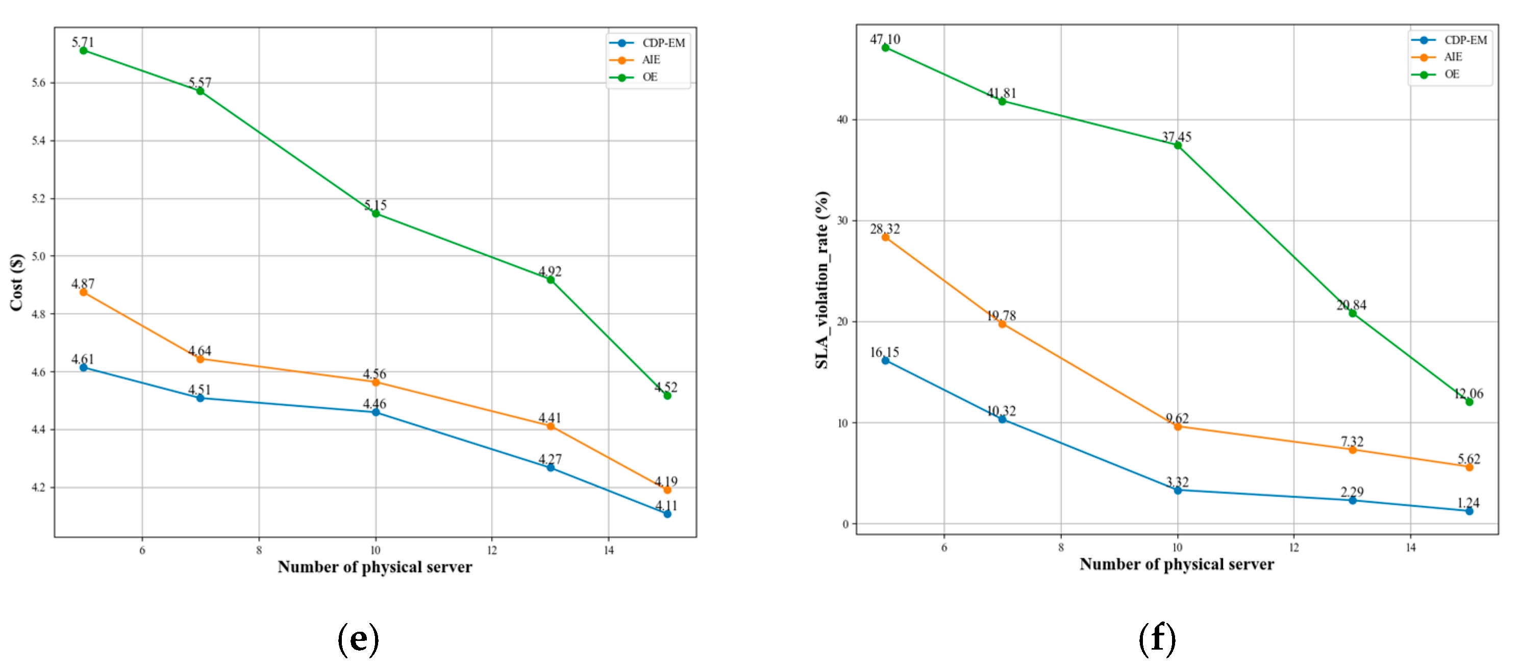
- Random [26]: Jobs are selected from the job queue and assigned with VM resources in a random manner.
- HEFT [13]: Prioritizes jobs for execution based on their estimated job completion times, taking into account both the computation and communication costs in a heterogeneous computing environment.
- PSO-MC [19]: A hybrid scheduling algorithm that integrates particle swarm optimization (PSO) with membrane computing (MC). It leverages job and resource states to determine the optimal scheduling solution, with the primary objective of minimizing the completion time and cost.
- DB-ACO [24]: An enhanced ant colony optimization (ACO) algorithm that is tailored for workflow scheduling in cloud environments. It incorporates deadline and budget constraints to ensure that the scheduling solution meets specific time and cost requirements.
- HCDRL [35]: A deep reinforcement learning-based cloud task scheduling strategy for multiple workflows. This strategy uses the continuity of task execution within workflows as a constraint, aiming at the performance, cost, and fairness of workflow tasks. The D3QN algorithm is employed to find the optimal solution. We have retained the performance and cost objectives of the tasks in this strategy.
- ATSIA3C [37]: A deep reinforcement learning-based cloud task scheduling strategy achieves a joint reduction in makespan and energy consumption through subtask granularity optimization. The A3C algorithm is employed to find the optimal solution. We have replaced the PPO algorithm used in our CDP-JS strategy with the A3C algorithm while retaining our scheduling strategy.
6.4. Hyperparameter Settings
6.5. Simulation Experiments
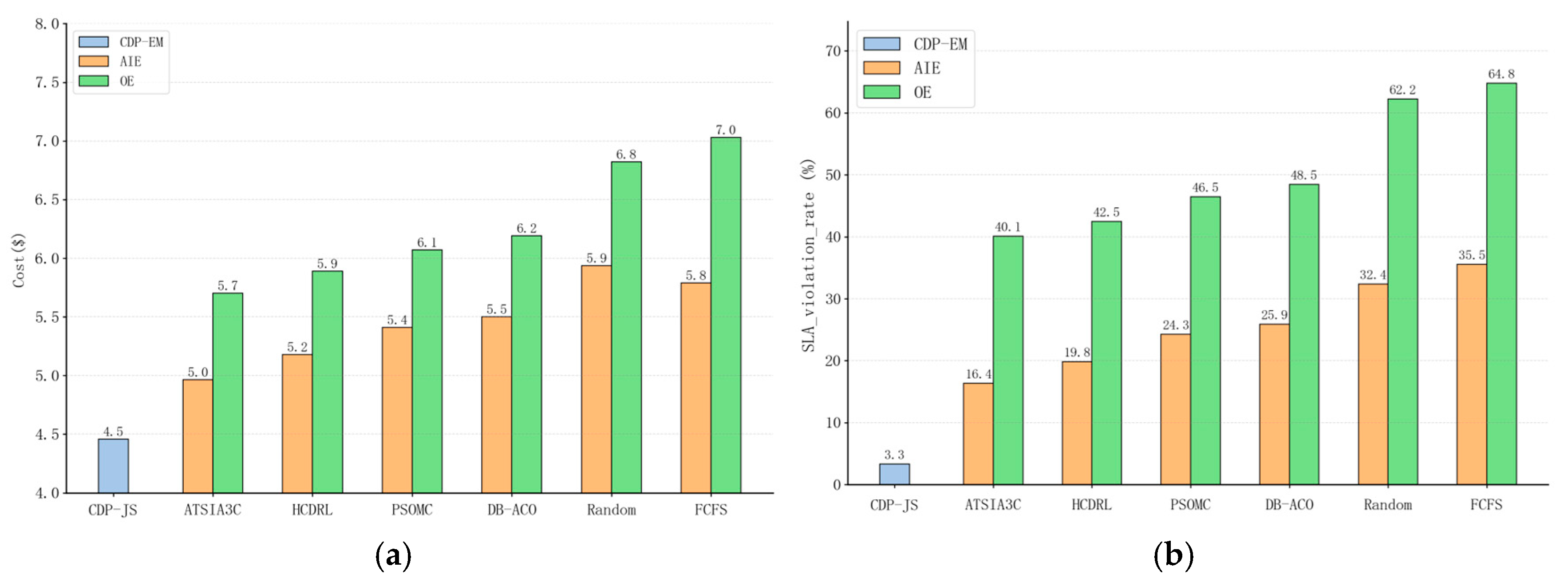
6.5.1. Overall Performance Evaluation
6.5.2. Performance Evaluation of CDP-EM
6.5.3. Performance Comparison of CDP-JS
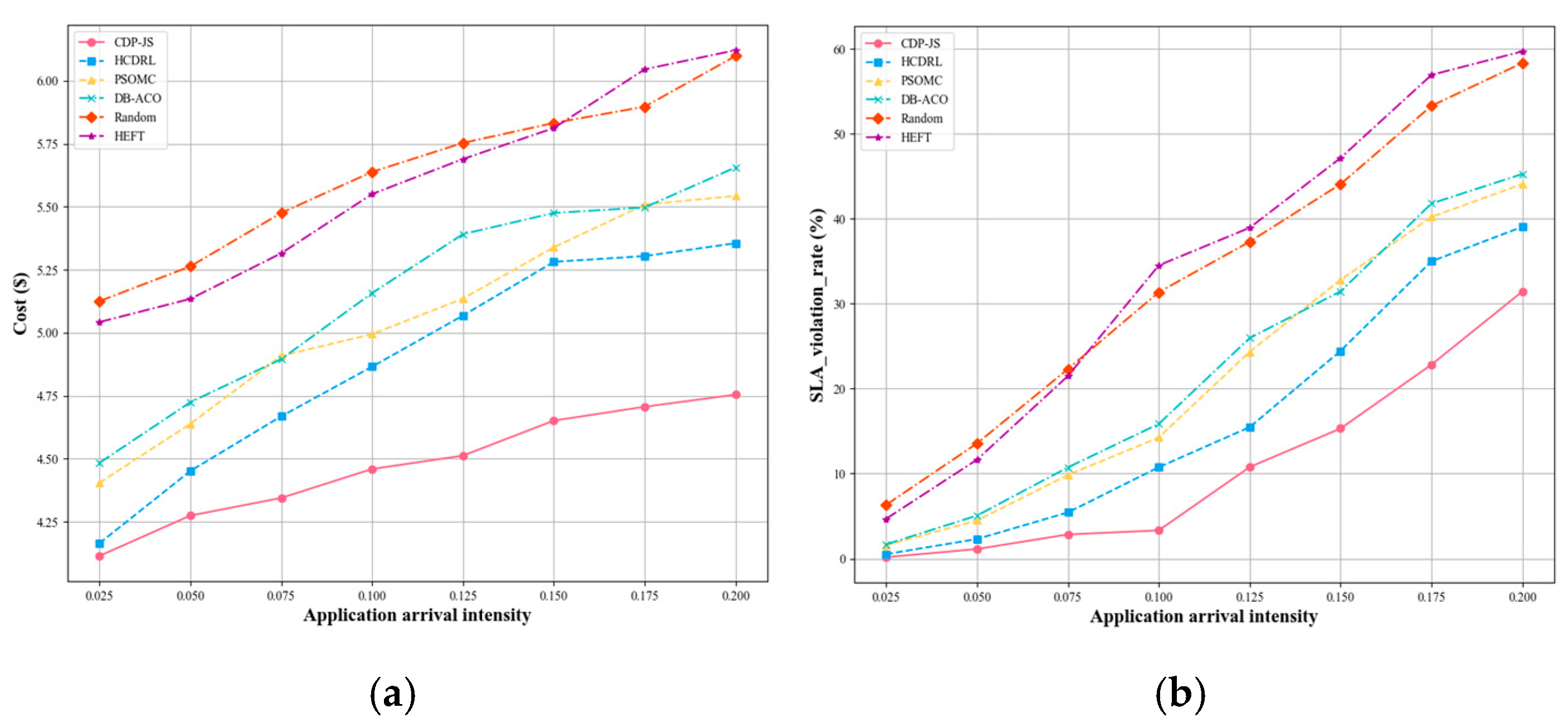
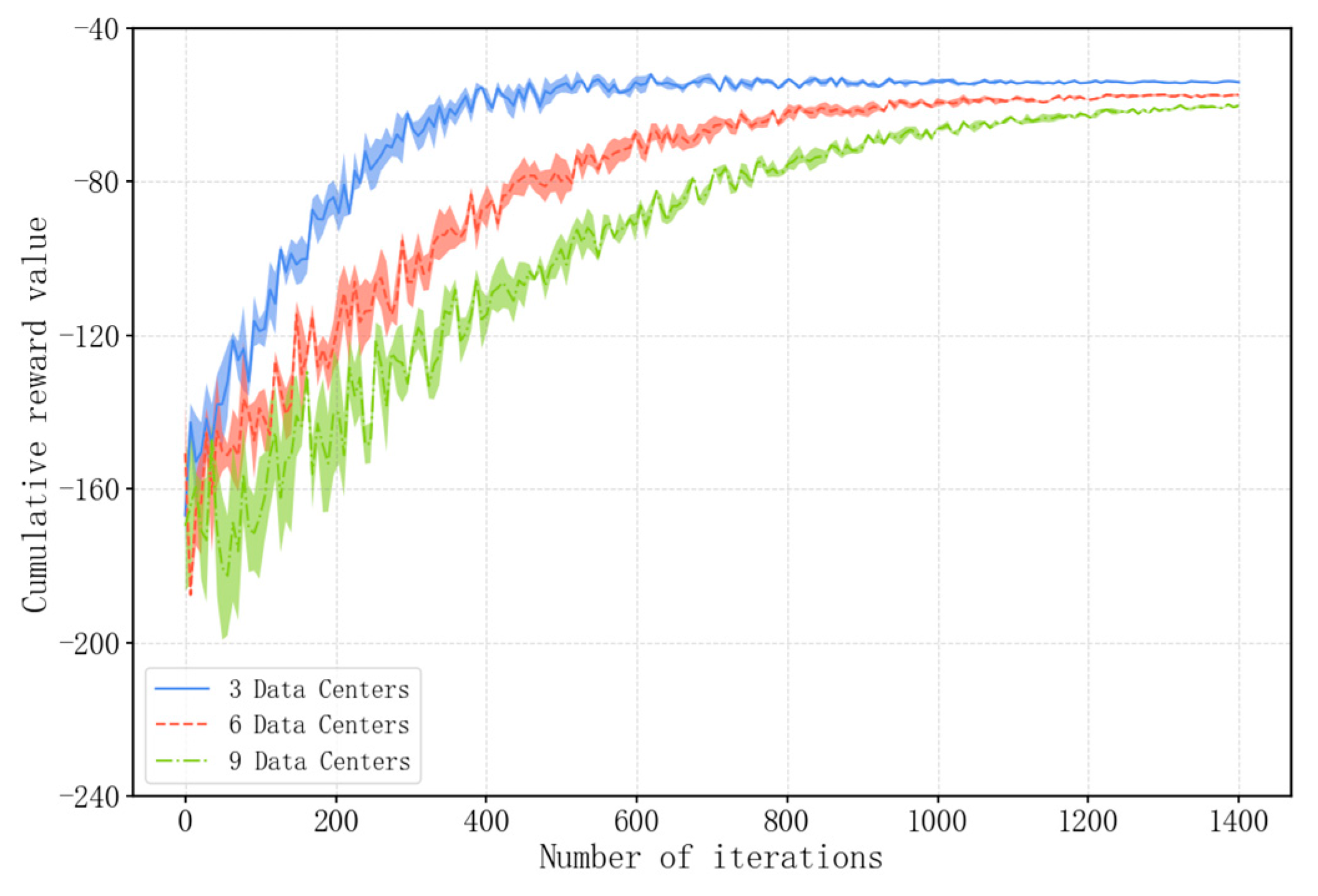
6.5.4. Scalability Study
6.5.5. Failure Resilience Study
6.6. Ablation Study
6.6.1. VM_Autoencoder
6.6.2. Req_Predictor
6.6.3. PPO Algorithm
6.6.4. Pretraining of Proposed PPO Algorithm
6.7. Real-World Experiments
7. Discussion
8. Conclusions
Author Contributions
Funding
Institutional Review Board Statement
Informed Consent Statement
Data Availability Statement
Conflicts of Interest
References
- Shakor, M.Y.; Khaleel, M.I. Recent Advances in Big Medical Image Data Analysis Through Deep Learning and Cloud Computing. Electronics 2024, 13, 4860. [Google Scholar] [CrossRef]
- Zhang, R.; Sun, Y.; Zhang, M. GPU-Based Genetic Programming for Faster Feature Extraction in Binary Image Classification. IEEE Trans. Evol. Computat. 2024, 28, 1590–1604. [Google Scholar] [CrossRef]
- González-San-Martín, J.; Martinez, F.; Smith, R. A Comprehensive Review of Task Scheduling Problem in Cloud Computing: Recent Advances and Comparative Analysis. New Horiz. Fuzzy Log. Neural Netw. Metaheuristics 2024, 1149, 299–313. [Google Scholar] [CrossRef]
- Shi, T.; Ma, H.; Chen, G.; Hartmann, S. Cost-Effective Web Application Replication and Deployment in Multi-Cloud Environment. IEEE Trans. Parallel Distrib. Syst. 2022, 33, 1982–1995. [Google Scholar] [CrossRef]
- Hou, H.; Agos Jawaddi, S.N.; Ismail, A. Energy Efficient Task Scheduling Based on Deep Reinforcement Learning in Cloud Environment: A Specialized Review. Future Gener. Comput. Syst. 2024, 151, 214–231. [Google Scholar] [CrossRef]
- Cai, X.; Geng, S.; Wu, D.; Cai, J.; Chen, J. A Multicloud-Model-Based Many-Objective Intelligent Algorithm for Efficient Task Scheduling in Internet of Things. IEEE Internet Things J. 2021, 8, 9645–9653. [Google Scholar] [CrossRef]
- Zhang, B.; Zeng, Z.; Shi, X.; Yang, J.; Veeravalli, B.; Li, K. A Novel Cooperative Resource Provisioning Strategy for Multi-Cloud Load Balancing. J. Parallel Distrib. Comput. 2021, 152, 98–107. [Google Scholar] [CrossRef]
- Tekawade, A.; Banerjee, S. A Cost Effective Reliability Aware Scheduler for Task Graphs in Multi-Cloud System. In Proceedings of the 2023 15th International Conference on COMmunication Systems & NETworkS (COMSNETS), Bangalore, India, 3–8 January 2023; pp. 295–303. [Google Scholar] [CrossRef]
- Tang, X. Reliability-Aware Cost-Efficient Scientific Workflows Scheduling Strategy on Multi-Cloud Systems. IEEE Trans. Cloud Comput. 2022, 10, 2909–2919. [Google Scholar] [CrossRef]
- Hu, H.; Li, Z.; Hu, H.; Chen, J.; Ge, J.; Li, C.; Chang, V. Multi-Objective Scheduling for Scientific Workflow in Multicloud Environment. J. Netw. Comput. Appl. 2018, 114, 108–122. [Google Scholar] [CrossRef]
- Xie, T.; Li, C.; Hao, N.; Luo, Y. Multi-Objective Optimization of Data Deployment and Scheduling Based on the Minimum Cost in Geo-Distributed Cloud. Comput. Commun. 2022, 185, 142–158. [Google Scholar] [CrossRef]
- Jiang, F.; Ferriter, K.; Castillo, C. A Cloud-Agnostic Framework to Enable Cost-Aware Scheduling of Applications in a Multi-Cloud Environment. In Proceedings of the NOMS 2020—2020 IEEE/IFIP Network Operations and Management Symposium, Budapest, Hungary, 20–24 April 2020; pp. 1–9. [Google Scholar] [CrossRef]
- Khan, Z.A.; Aziz, I.A.; Osman, N.A.B.; Ullah, I. A Review on Task Scheduling Techniques in Cloud and Fog Computing: Taxonomy, Tools, Open Issues, Challenges, and Future Directions. IEEE Access 2023, 11, 143417–143445. [Google Scholar] [CrossRef]
- Kanbar, A.B.; Faraj, K. Region Aware Dynamic Task Scheduling and Resource Virtualization for Load Balancing in IoT–Fog Multi-Cloud Environment. Future Gener. Comput. Syst. 2022, 137, 70–86. [Google Scholar] [CrossRef]
- Zhou, X.; Zhang, G.; Sun, J.; Zhou, J.; Wei, T.; Hu, S. Minimizing Cost and Makespan for Workflow Scheduling in Cloud Using Fuzzy Dominance Sort Based HEFT. Future Gener. Comput. Syst. 2019, 93, 278–289. [Google Scholar] [CrossRef]
- Alam, A.B.M.B.; Fadlullah, Z.M.; Choudhury, S. A Resource Allocation Model Based on Trust Evaluation in Multi-Cloud Environments. IEEE Access 2021, 9, 105577–105587. [Google Scholar] [CrossRef]
- Liu, Z.; Xiang, T.; Lin, B.; Ye, X.; Wang, H.; Zhang, Y.; Chen, X. A Data Placement Strategy for Scientific Workflow in Hybrid Cloud. In Proceedings of the 2018 IEEE 11th International Conference on Cloud Computing (CLOUD), San Francisco, CA, USA, 2–7 July 2018; pp. 556–563. [Google Scholar] [CrossRef]
- Meena, J.; Kumar, M.; Vardhan, M. Cost Effective Genetic Algorithm for Workflow Scheduling in Cloud Under Deadline Constraint. IEEE Access 2016, 4, 5065–5082. [Google Scholar] [CrossRef]
- Li, K.; Jia, L.; Shi, X. Research on Cloud Computing Task Scheduling Based on PSOMC. J. Web Eng. 2022, 21, 1749–1766. [Google Scholar] [CrossRef]
- Shi, T.; Ma, H.; Chen, G. A Genetic-Based Approach to Location-Aware Cloud Service Brokering in Multi-Cloud Environment. In Proceedings of the 2019 IEEE International Conference on Services Computing (SCC), Milan, Italy, 8–13 July 2019; pp. 146–153. [Google Scholar] [CrossRef]
- Nabi, S.; Ahmad, M.; Ibrahim, M.; Hamam, H. AdPSO: Adaptive PSO-Based Task Scheduling Approach for Cloud Computing. Sensors 2022, 22, 920. [Google Scholar] [CrossRef]
- Talha, A.; Malki, M.O.C. PPTS-PSO: A New Hybrid Scheduling Algorithm for Scientific Workflow in Cloud Environment. Multimed. Tools Appl. 2023, 82, 33015–33038. [Google Scholar] [CrossRef]
- Kaur, A.; Singh, P.; Singh Batth, R.; Peng Lim, C. Deep-Q Learning-based Heterogeneous Earliest Finish Time Scheduling Algorithm for Scientific Workflows in Cloud. Softw. Pract. Exp. 2022, 52, 689–709. [Google Scholar] [CrossRef]
- Tao, S.; Xia, Y.; Ye, L.; Yan, C.; Gao, R. DB-ACO: A Deadline-Budget Constrained Ant Colony Optimization for Workflow Scheduling in Clouds. IEEE Trans. Automat. Sci. Eng. 2024, 21, 1564–1579. [Google Scholar] [CrossRef]
- Ullah, A.; Alomari, Z.; Alkhushayni, S.; Al-Zaleq, D.A.; Bany Taha, M.; Remmach, H. Improvement in task allocation for VM and reduction of Makespan in IaaS model for cloud computing. Clust. Comput. 2024, 27, 11407–11426. [Google Scholar] [CrossRef]
- Wang, H.; Wang, H. Survey On Task Scheduling in Cloud Computing Environment. In Proceedings of the 2022 7th International Conference on Intelligent Informatics and Biomedical Science (ICIIBMS), Nara, Japan, 24–26 November 2022; pp. 286–291. [Google Scholar] [CrossRef]
- Mao, H.; Schwarzkopf, M.; Venkatakrishnan, S.B.; Meng, Z.; Alizadeh, M. Learning Scheduling Algorithms for Data Processing Clusters. In Proceedings of the ACM Special Interest Group on Data Communication, Beijing, China, 19–23 August 2019; ACM: New York, NY, USA, 2019; pp. 270–288. [Google Scholar] [CrossRef]
- Wang, P.; Xie, X.; Guo, X. Research on Resource Scheduling Algorithm for The Cloud. In Proceedings of the 2021 International Conference on Intelligent Transportation, Big Data & Smart City (ICITBS), Xi’an, China, 27–28 March 2021; pp. 732–735. [Google Scholar]
- Guo, X. Multi-Objective Task Scheduling Optimization in Cloud Computing Based on Fuzzy Self-Defense Algorithm. Alex. Eng. J. 2021, 60, 5603–5609. [Google Scholar] [CrossRef]
- Qin, Y.; Wang, H.; Yi, S.; Li, X.; Zhai, L. A Multi-Objective Reinforcement Learning Algorithm for Deadline Constrained Scientific Workflow Scheduling in Clouds. Front. Comput. Sci. 2021, 15, 155105. [Google Scholar] [CrossRef]
- Zhao, F.A. Resource Scheduling Method Based on Deep Reinforcement Learning. Comput. Sci. Appl. 2021, 11, 2008–2018. [Google Scholar] [CrossRef]
- Li, F.; Hu, B. DeepJS: Job Scheduling Based on Deep Reinforcement Learning in Cloud Data Center. In Proceedings of the Proceedings of the 2019 4th International Conference on Big Data and Computing—ICBDC 2019, Guangzhou, China, 10–12 May 2019; ACM Press: New York, NY, USA; pp. 48–53. [Google Scholar]
- Mondal, S.S.; Sheoran, N.; Mitra, S. Scheduling of Time-Varying Workloads Using Reinforcement Learning. AAAI 2021, 35, 9000–9008. [Google Scholar] [CrossRef]
- Ran, L.; Shi, X.; Shang, M. SLAs-Aware Online Task Scheduling Based on Deep Reinforcement Learning Method in Cloud Environment. In Proceedings of the IEEE 5th International Conference on Data Science and Systems (DSS), Zhangjiajie, China, 10–12 August 2019; pp. 1518–1525. [Google Scholar]
- Chen, G.; Qi, J.; Sun, Y.; Hu, X.; Dong, Z.; Sun, Y. A Collaborative Scheduling Method for Cloud Computing Heterogeneous Workflows Based on Deep Reinforcement Learning. Future Gener. Comput. Syst. 2023, 141, 284–297. [Google Scholar] [CrossRef]
- Zhang, S.; Zhao, Z.; Liu, C.; Qin, S. Data-intensive workflow scheduling strategy based on deep reinforcement learning in multi-clouds. J. Cloud Comp. 2023, 12, 125. [Google Scholar] [CrossRef]
- Mangalampalli, S.; Karri, G.R.; Ratnamani, M.V.; Mohanty, S.N.; Jabr, B.A.; Ali, Y.A.; Ali, S.; Abdullaeva, B.S. Efficient deep reinforcement learning based task scheduler in multi cloud environment. Sci. Rep. 2024, 14, 21850. [Google Scholar] [CrossRef]
- Abraham, O.L.; Ngadi, M.A.B.; Sharif, J.B.M.; Sidik, M.K.M. Multi-Objective Optimization Techniques in Cloud Task Scheduling: A Systematic Literature Review. IEEE Access 2025, 13, 12255–12291. [Google Scholar] [CrossRef]
- Zhang, X.; Zhu, G.-Y. A Literature Review of Reinforcement Learning Methods Applied to Job-Shop Scheduling Problems. Comput. Oper. Res. 2025, 175, 106929. [Google Scholar] [CrossRef]
- AWS. Amazon EC2 On-Demand Data Transfer Pricing [EB/OL]. Available online: https://aws.amazon.com/cn/ec2/pricing/on-demand/ (accessed on 5 March 2025).
- Microsoft Azure. Bandwidth Pricing [EB/OL]. Available online: https://azure.microsoft.com/zh-cn/pricing/details/bandwidth/ (accessed on 5 March 2025).
- Schulman, J.; Moritz, P.; Levine, S.; Jordan, M.I.; Abbeel, P. Proximal Policy Optimization Algorithms. arXiv 2017, arXiv:1707.06347. [Google Scholar]
- Ming, F.; Gong, W.; Wang, L.; Jin, Y. Constrained Multi-Objective Optimization with Deep Reinforcement Learning Assisted Operator Selection. IEEE/CAA J. Autom. Sin. 2024, 11, 919–931. [Google Scholar] [CrossRef]
- Xu, M.; Song, C.; Wu, H.; Gill, S.S.; Ye, K.; Xu, C. esDNN: Deep Neural Network Based Multivariate Workload Prediction in Cloud Computing Environments. ACM Trans. Internet Technol. 2022, 22, 1–24. [Google Scholar] [CrossRef]
- Liang, R.; Xie, X.; Zhai, Q.; Zhang, Q. Study on Container Cloud Load Prediction Based on Improved Stacking Integration Model. Comput. Appl. Softw. 2023, 40, 48–100. [Google Scholar]
- Dang, W.; Zhou, B.; Wei, L.; Zhang, W.; Yang, Z.; Hu, S. TS-Bert: Time Series Anomaly Detection via Pre-Training Model Bert. In Computational Science—ICCS 2021; Lecture Notes in Computer Science; Springer International Publishing AG: Cham, Switzerland, 2021; Volume 12743, pp. 209–223. [Google Scholar] [CrossRef]
- Alibaba Inc. Cluster Data Collected from Production Clusters in Alibaba for Cluster Management Research. 2018. Available online: https://github.com/alibaba/clusterdata (accessed on 15 February 2025).
- Rio, A.D.; Jimenez, D.; Serrano, J. Comparative Analysis of A3C and PPO Algorithms in Reinforcement Learning: A Survey on General Environments. IEEE Access 2024, 12, 146795–146806. [Google Scholar]
- BenchCouncil. BigDataBench [EB/OL]. Available online: https://www.benchcouncil.org/BigDataBench/index.html (accessed on 5 March 2025).
- Ramos, G. E-commerce Business Transaction Sales Data. Kaggle. 2023. Available online: https://www.kaggle.com/datasets/gabrielramos87/an-online-shop-business (accessed on 15 February 2025).
- Sogu Data Collection: Multimodal Social Media Analytics. 2023. Available online: https://www.selectdataset.com/dataset/966d4417a510d32a8423f2da627c342a (accessed on 15 February 2025).
- Harper, F.M.; Konstan, J.A. The MovieLens datasets: History and context. ACM Trans. Interact. Intell. Syst. 2015, 5, 19. [Google Scholar] [CrossRef]
- Facebook Social Network Dataset; Stanford University: Stanford, CA, USA, 2024; Available online: https://github.com/emreokcular/social-circle (accessed on 12 March 2024).
- Kaur, A.; Dhiman, A.; Singh, M. Comprehensive Review: Security Challenges and Countermeasures for Big Data Security in Cloud Computing. In Proceedings of the 2023 7th International Conference on Electronics, Materials Engineering & Nano-Technology (IEMENTech), Kolkata, India, 18–20 December 2023; pp. 1–6. [Google Scholar]
- Sreekumari, P. Privacy-Preserving Keyword Search Schemes over Encrypted Cloud Data: An Extensive Analysis. In Proceedings of the 2018 IEEE 4th International Conference on Big Data Security on Cloud (BigDataSecurity), IEEE International Conference on High Performance and Smart Computing, (HPSC) and IEEE International Conference on Intelligent Data and Security (IDS), Omaha, NE, USA, 3–5 May 2018; pp. 114–120. [Google Scholar]
- Soni, V.; Jain, V.; Santhoshkumar, G.P. Secure Communication Protocols for IoT-Enabled Smart Grids. In Proceedings of the 2024 International Conference on Innovative Computing, Intelligent Communication and Smart Electrical Systems (ICSES), Chennai, India, 12–13 December 2024; pp. 1–6. [Google Scholar]
- Vineela, A.; Kasiviswanath, N.; Bindu, C.S. Data Integrity Auditing Scheme for Preserving Security in Cloud Based Big Data. In Proceedings of the 2022 6th International Conference on Intelligent Computing and Control Systems (ICICCS), Madurai, India, 25–27 May 2022; pp. 609–613. [Google Scholar]
- Emara, T.Z.; Huang, J.Z. Distributed Data Strategies to Support Large-Scale Data Analysis Across Geo-Distributed Data Centers. IEEE Access 2020, 8, 178526–178538. [Google Scholar] [CrossRef]
- Choudhary, A.; Verma, P.K.; Rai, P. Comparative Study of Various Cloud Service Providers: A Review. In Proceedings of the 2022 International Conference on Power, Energy, Control and Transmission Systems (ICPECTS), Chennai, India, 8–9 December 2022; pp. 1–8. [Google Scholar]
- Zhu, Z.; Lin, K.; Jain, A.K.; Zhou, J. Transfer Learning in Deep Reinforcement Learning: A Survey. IEEE Trans. Pattern Anal. Mach. Intell. 2023, 45, 13344–13362. [Google Scholar] [CrossRef]


| Data Center | VM Type | vCPU | Mem (GB) | Computing Power (GFLOPS) | Per Hour ($) |
|---|---|---|---|---|---|
| Center 1 | a1.small | 2 | 8.60 | 35.2 | 0.0832 |
| a1.middle | 4 | 17.18 | 70.4 | 0.166 | |
| a1.large | 8 | 34.36 | 140.8 | 0.333 | |
| a1.xlarge | 16 | 68.72 | 281.6 | 0.666 | |
| Center 2 | b1.small | 2 | 8.59 | 36.8 | 0.0816 |
| b1.middle | 4 | 17.18 | 73.6 | 0.1632 | |
| b1.large | 8 | 34.36 | 147.2 | 0.3264 | |
| b1.xlarge | 16 | 64.00 | 294.4 | 0.6528 | |
| Center 3 | c1.small | 2 | 1.80 | 40 | 0.0709 |
| c1.middle | 4 | 3.60 | 80 | 0.1418 | |
| c1.large | 8 | 7.21 | 160 | 0.2836 | |
| c1.xlarge | 16 | 14.42 | 320 | 0.5672 |
| Data Center | Cluster Type | Cluster Number | CPU Core Number | Core Computing Power (GFLOPS) | Mem (GB) |
|---|---|---|---|---|---|
| Center 1 | Cluster1 | 10 | 50 | 35.2 | 161 |
| Center 2 | Cluster2 | 10 | 50 | 36.8 | 161 |
| Center 3 | Cluster3 | 10 | 50 | 40 | 40 |
| Source Data Center | Destination Data Center | Bandwidth |
|---|---|---|
| Center 1 | Center 2 | 800 Mbps |
| Center 2 | Center 3 | 600 Mbps |
| Center 1 | Center 3 | 1 Gbps |
| Algorithm | Hyperparameters | Parameter Values |
|---|---|---|
| PPO Network (DC_Encoder+Act_Dec) | Discount Factor | 0.95 |
| Actor Learning Rate | 0.0001 | |
| Critic Learning Rate | 0.0002 | |
| GAE Lambda | 0.95 | |
| Clip Parameter | 0.2 | |
| Batch Size | 128 | |
| VM_Autoencoder | Learning Rate | 0.001 |
| Kernel Regularization | L2 | |
| Internal layer Activation Function | ReLu | |
| Output layer Activation Function | Sigmoid | |
| Optimizer | Adam | |
| Epochs | 500 | |
| Batch Size | 32 | |
| Req_Predictor | Learning Rate | 0.001 |
| Input Dimension | 5 | |
| Hidden Units | 32 | |
| Layers | 2 | |
| Epochs | 500 | |
| Batch Size | 32 |
| ID | No. of Data Centers | New VM Type | New VM Location | VM Price Variation | CDP Application Arrival Intensity |
|---|---|---|---|---|---|
| #2 | 6 | d1. Micro, d1.xxlarge | 3 | 1.2 | 0.2 |
| #3 | 9 | d1. Micro, d1.xxlarge e1. Micro, e1.xxlarge | 4 | 1.4 | 0.3 |
| Data Center | VM Type | vCPU | Mem (GB) | Computing Power (GFLOPS) | Per Hour ($) |
|---|---|---|---|---|---|
| Center 4, 5, 6 | d1. micro | 1 | 4.30 | 17.6 | 0.0416 |
| d1.xxlarge | 24 | 103.08 | 422.4 | 0.999 | |
| Center 7, 8, 9 | e1. micro | 1 | 4.30 | 18.4 | 0.0408 |
| e1.xxlarge | 24 | 103.08 | 441.6 | 0.9792 |
| CDP-JS | HCDRL | PSOMC | DB-ACO | Random | FCFS | ||
|---|---|---|---|---|---|---|---|
| 10% VM interruption | Cost ($) | 4.918 | 5.362 | 5.477 | 5.681 | 6.216 | 6.246 |
| SLA_violation_rate (%) | 4.60 | 14.83 | 19.39 | 21.19 | 43.89 | 46.63 | |
| 20% VM interruption | Cost ($) | 5.456 | 5.918 | 6.142 | 6.261 | 6.893 | 6.754 |
| SLA_violation_rate (%) | 5.78 | 17.79 | 24.25 | 25.74 | 48.94 | 49.87 | |
| Original | Ablation | |
|---|---|---|
| Cost ($) | 4.359 | 4.442 |
| SLA_violation_rate(%) | 5.32 | 7.20 |
| Original | Ablation_Str+Input | Ablation_Str | |
|---|---|---|---|
| Cost ($) | 4.359 | 4.474 | 4.428 |
| SLA_violation_rate (%) | 5.32 | 8.60 | 8.2 |
| Original | Ablation_D3QN | |
|---|---|---|
| Cost ($) | 4.359 | 4.486 |
| SLA_violation_rate (%) | 5.32 | 10.76 |
| Data Center | VM Type | vCPU | Mem (GB) | Computing Power (GFLOPS) | Per Hour ($) |
|---|---|---|---|---|---|
| BCC | a1.small | 2 | 8 | 36.8 | 0.0832 |
| a1.middle | 4 | 16 | 73.6 | 0.166 | |
| a1.large | 8 | 32 | 147.2 | 0.333 | |
| a1.xlarge | 12 | 64 | 220.8 | 0.666 | |
| ICT | b1.small | 2 | 8 | 33.6 | 0.0816 |
| b1.middle | 4 | 16 | 67.2 | 0.1632 | |
| b1.large | 8 | 32 | 134.4 | 0.3264 | |
| b1.xlarge | 12 | 64 | 201.6 | 0.6528 | |
| NISB | c1.small | 2 | 8 | 35.2 | 0.0709 |
| c1.middle | 4 | 12 | 70.4 | 0.1418 | |
| c1.large | 8 | 32 | 140.8 | 0.2836 | |
| c1.xlarge | 12 | 64 | 211.2 | 0.5672 |
| Source Data Center | Destination Data Center | Bandwidth |
|---|---|---|
| BCC | ICT | 8 Gbps |
| BCC | NISB | 4 Gbps |
| ICT | NISB | 10 Gbps |
| Application Name | Preprocessing Stage | Aggregate Analysis Stage | Dataset |
|---|---|---|---|
| E-commerce Customer Behavior Analysis | Grep: Identifying Target User Group | K-Means: Customer Classification | E-Commerce Transaction Data [50] |
| Web Page Indexing | WordCount: Webpage Keyword Extraction | H-Index: Webpage Indexing | Sogu Data [51] |
| Movie Recommendation | Filter: Removing Invalid Records | CF: Collaborative Filtering Recommendation | MovieLen Data [52] |
| Community Discovery | Select Query: Selecting Key Attributes | Connected Component: Community Detection | Facebook Social Network Data [53] |
| CDP-JS | HCDRL | PSOMC | DB-ACO | Random | FCFS | |
|---|---|---|---|---|---|---|
| Cost ($) | 5.832 | 7.579 | 8.532 | 8.619 | 9.021 | 8.835 |
| SLA_violation_rate (%) | 4.58 | 24.32 | 27.68 | 28.42 | 38.32 | 40.32 |
Disclaimer/Publisher’s Note: The statements, opinions and data contained in all publications are solely those of the individual author(s) and contributor(s) and not of MDPI and/or the editor(s). MDPI and/or the editor(s) disclaim responsibility for any injury to people or property resulting from any ideas, methods, instructions or products referred to in the content. |
© 2025 by the authors. Licensee MDPI, Basel, Switzerland. This article is an open access article distributed under the terms and conditions of the Creative Commons Attribution (CC BY) license (https://creativecommons.org/licenses/by/4.0/).
Share and Cite
Liang, Y.; Xu, G.; Shen, H.; Ruan, N.; Wang, Y. Towards Efficient Job Scheduling for Cumulative Data Processing in Multi-Cloud Environments. Electronics 2025, 14, 1332. https://doi.org/10.3390/electronics14071332
Liang Y, Xu G, Shen H, Ruan N, Wang Y. Towards Efficient Job Scheduling for Cumulative Data Processing in Multi-Cloud Environments. Electronics. 2025; 14(7):1332. https://doi.org/10.3390/electronics14071332
Chicago/Turabian StyleLiang, Yi, Guimei Xu, Haotian Shen, Nianyi Ruan, and Yinzhou Wang. 2025. "Towards Efficient Job Scheduling for Cumulative Data Processing in Multi-Cloud Environments" Electronics 14, no. 7: 1332. https://doi.org/10.3390/electronics14071332
APA StyleLiang, Y., Xu, G., Shen, H., Ruan, N., & Wang, Y. (2025). Towards Efficient Job Scheduling for Cumulative Data Processing in Multi-Cloud Environments. Electronics, 14(7), 1332. https://doi.org/10.3390/electronics14071332