Author Contributions
Conceptualization, J.C.; methodology, J.C.; software, J.C.; validation, J.C.; formal analysis, J.C.; investigation, J.C.; resources, J.C.; data curation, J.C.; writing—original draft preparation, J.C.; writing—review and editing, J.C. and X.T.; visualization, J.C.; supervision, C.D.; project administration, C.D.; funding acquisition, C.D. All authors have read and agreed to the published version of the manuscript.
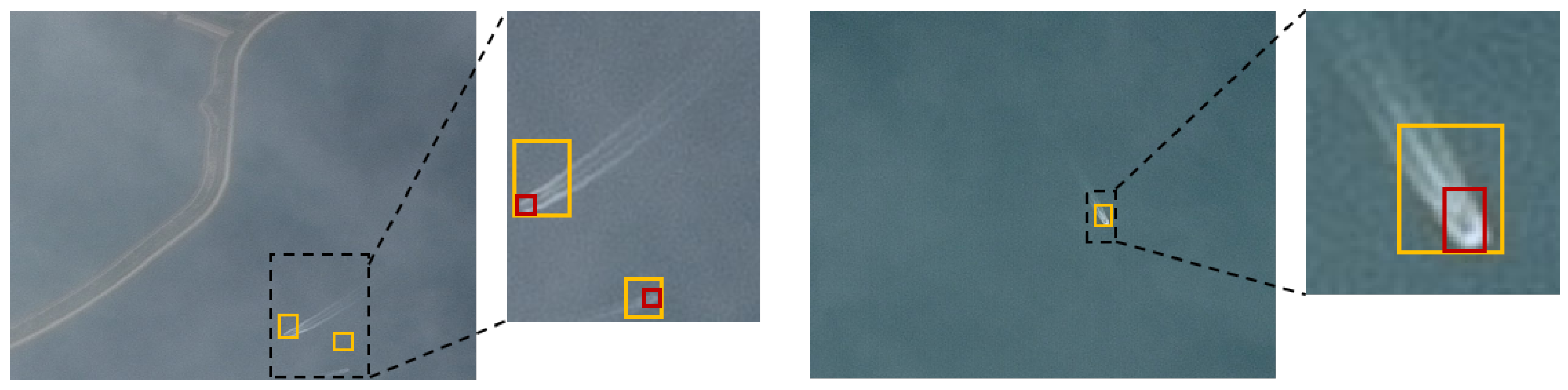
Figure 1.
Optical RS ship detection examples at 16 m resolution. The yellow box denotes the annotated bounding box, while the red box delineates the actual ship boundary. As can be observed, due to the limited image resolution, ship targets occupy only a few pixels. Additionally, there are discrepancies between the manually annotated bounding boxes and the actual ship boundaries.
Figure 2.
The overall structure of DPCSANet. Backbone: CSPDarknet53 is used as the backbone network to efficiently extract features and use the high-dimensional hybrid multiscale pooling module to expand the feature fusion range. Neck: A simplified bidirectional feature fusion network (PAN) is used, and DPBlock containing a dual-path convolutional self-attention mechanism is introduced to enhance the model’s ability to extract contextual information of the target and surrounding features. Considering the computational complexity and prediction recall rate of the model, three-layer detection branches , , and are used to predict ships of different sizes. Head: Focal CIoU regression loss function is used to improve the detection recall rate.
Figure 3.
Illustration of the perceptual capabilities and feature extraction paths of CNNs, self-attention mechanisms, self-attention with convolution, and the proposed dual-path convolutional self-attention (DPCSA). Different colored arrows indicate independent feature extraction paths for each mechanism. CNNs capture local features through limited receptive fields, focusing primarily on local textures. Self-attention mechanisms capture global dependencies, allowing each position to interact with all other positions in the input. Self-attention with convolution combines both local and global feature extraction but often concatenates these features in the same channel, potentially leading to interference. In contrast, DPCSA parallelizes convolution and self-attention mechanisms, processing them independently to avoid interference. This design maximizes the extraction of both local and global features within a single feature map, enhancing the model’s ability to distinguish between target and background features.
![Electronics 14 01225 g003]()
Figure 4.
The overall structure of DPBlock and the principle of DPCSA. DPCSA consists of two branches, using a multi-head self-attention mechanism [
18] and two-dimensional convolution to extract global and local features, respectively. Among them, the local features are weighted using the learnable parameter
and then fused with the global features extracted by the self-attention mechanism.
Figure 5.
The structure of HHSPP.
Figure 5.
The structure of HHSPP.
Figure 6.
Samples of (a) LEVIR-ship and (b) OSSD datasets.
Figure 6.
Samples of (a) LEVIR-ship and (b) OSSD datasets.
Figure 7.
Schematic illustration of the process for extracting and cropping ship samples from the DOTA dataset. The original images are segmented into 640 × 640 patches with a 200-pixel overlap, and only those containing ship targets are retained and re-labeled to form the DOTA-ship dataset.
Figure 7.
Schematic illustration of the process for extracting and cropping ship samples from the DOTA dataset. The original images are segmented into 640 × 640 patches with a 200-pixel overlap, and only those containing ship targets are retained and re-labeled to form the DOTA-ship dataset.
Figure 8.
Distribution of ship label length and width in different datasets. Different colors represent varying probability values, with lighter colors indicating higher probabilities of ship label occurrence. (a) LEVIR-ship, (b) OSSD, and (c) DOTA-ship.
Figure 8.
Distribution of ship label length and width in different datasets. Different colors represent varying probability values, with lighter colors indicating higher probabilities of ship label occurrence. (a) LEVIR-ship, (b) OSSD, and (c) DOTA-ship.
Figure 9.
Some detection results of the proposed DPCSANet on LEVIR-ship. The red boxes represent the ground truth annotations, while the blue boxes indicate the predicted bounding boxes.
Figure 9.
Some detection results of the proposed DPCSANet on LEVIR-ship. The red boxes represent the ground truth annotations, while the blue boxes indicate the predicted bounding boxes.
Figure 10.
Some detection results of the proposed DPCSANet on OSSD. The red boxes represent the ground truth annotations, while the blue boxes indicate the predicted bounding boxes.
Figure 10.
Some detection results of the proposed DPCSANet on OSSD. The red boxes represent the ground truth annotations, while the blue boxes indicate the predicted bounding boxes.
Figure 11.
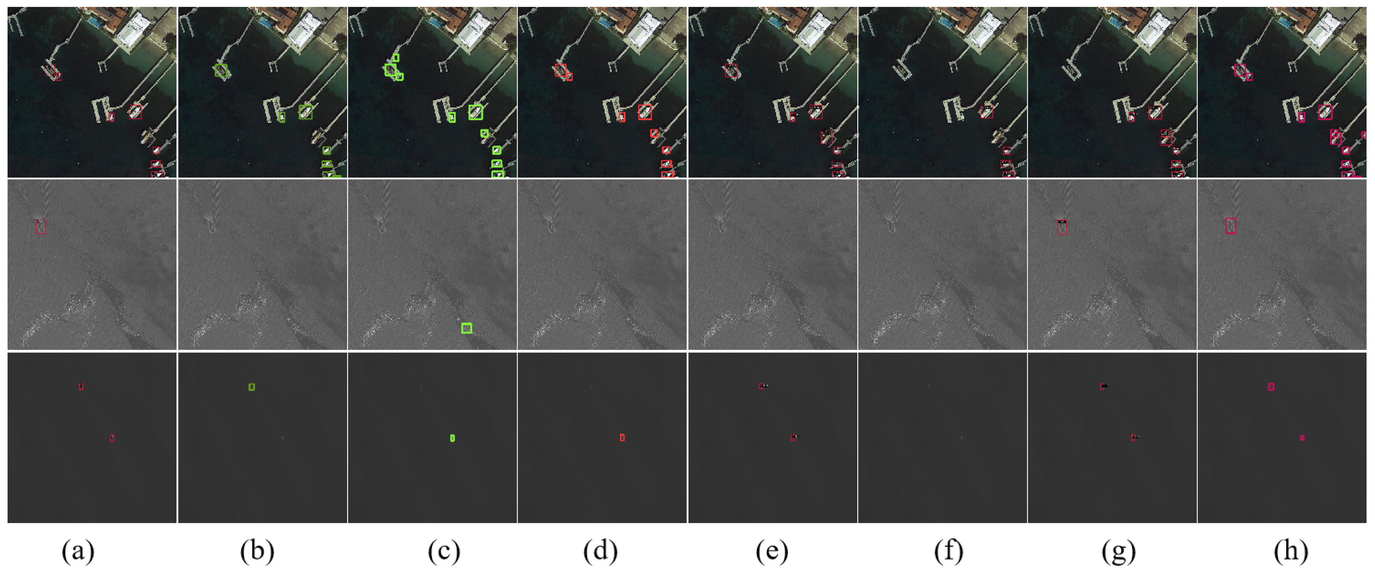
Comparison of the detection results on DOTA-ship for different methods. (a) Ground truth; (b) YOLOv5s (baseline); (c) YOLOv7; (d) YOLOv9; (e) cascade RCNN; (f) RetinaNet; (g) DINO; (h) DPCSANet (ours).
Figure 11.
Comparison of the detection results on DOTA-ship for different methods. (a) Ground truth; (b) YOLOv5s (baseline); (c) YOLOv7; (d) YOLOv9; (e) cascade RCNN; (f) RetinaNet; (g) DINO; (h) DPCSANet (ours).
Figure 12.
Influence of DPCSA, HHSPP, and Focal CIoU on feature extraction. The brighter color represents that the model pays more attention to that area.
Figure 12.
Influence of DPCSA, HHSPP, and Focal CIoU on feature extraction. The brighter color represents that the model pays more attention to that area.
Figure 13.
Samples of three different scenes: clear scene, fractus or mist conditions, and thick fog or thick cloud conditions.
Figure 13.
Samples of three different scenes: clear scene, fractus or mist conditions, and thick fog or thick cloud conditions.
Figure 14.
Examples of false positives and false negatives in DPCSANet testing. The red mark indicates false positives caused by cloud interference and ground structure classification errors. Yellow indicates missed detection, i.e., false negative. Some small ship targets were not detected due to their limited size and weak feature representation.
Table 1.
Comparison with state-of-the-art methods on the LEVIR-ship dataset. The optimal result is represented in bold font.
Table 1.
Comparison with state-of-the-art methods on the LEVIR-ship dataset. The optimal result is represented in bold font.
| Model | Backbone | Params/M | FLOPs/G | FPS | P/% | R/% | AP/% |
|---|
| YOLOv5s [25] | - | 7.05 | 10.4 | 208 | 58.7 | 81.9 | 73.6 |
| YOLOv7tiny [26] | - | 6.01 | 13 | 256 | 71.8 | 65.9 | 65.2 |
| YOLOv7l | - | 36.48 | 103.2 | 127 | 77.4 | 71.6 | 69.8 |
| YOLOv7x | - | 70.78 | 188 | 78 | 76.9 | 63.2 | 70.4 |
| YOLOv8n | | 3.01 | 8.1 | 222 | 73.3 | 63.6 | 67.4 |
| YOLOv8s | - | 11.13 | 28.4 | 185 | 79.2 | 71.9 | 75.1 |
| YOLOv8m | - | 25.84 | 78.7 | 96 | 78 | 72.6 | 72.0 |
| YOLOv8l | - | 43.61 | 164.8 | 54 | 77.2 | 71.4 | 74.0 |
| YOLOv9c [27] | - | 50.70 | 236.6 | 33 | 76.7 | 71.7 | 73.1 |
| YOLOv9e | - | 68.55 | 240.7 | 26 | 78.8 | 75.9 | 78.5 |
| Faster RCNN [23] | VGG16 | 136.7 | 299.2 | 34 | - | - | 70.8 |
| CenterNet [48] | Hourglass-104 | 191.2 | 584.6 | 35 | - | - | 77.7 |
| RT-DETR [50] | ResNet50 | 42 | 136 | 29 | - | - | 70.9 |
| | ResNet101 | 76 | 259 | 22 | - | - | 73.9 |
| Cascade RCNN [49] | ResNet50 | 69.15 | 162 | 22 | - | - | 81.2 |
| | ResNet101 | 88.14 | 209 | 18 | - | - | 81.3 |
| DINO [51] | ResNet50 | 47.54 | 179 | 16 | - | - | 83.8 |
| DRENet [17] | - | 4.79 | 8.4 | 169 | 52.7 | 86.0 | 81.7 |
| ImYOLOv5 [31] | - | 8.64 | 16.7 | 139 | 42.1 | 86.5 | 78.9 |
| FFCA-YOLO [43] | - | 71.22 | 51.2 | 113 | 75.9 | 63.8 | 62.8 |
| Imyolov8 [52] | - | 5.31 | 55.0 | 135 | 75.2 | 68.2 | 67.6 |
| DPCSANet (Ours) | - | 6.20 | 9.6 | 149 | 66.1 | 88.2 | 85.0 |
Table 2.
Comparison with the state-of-the-art methods on the OSSD dataset. The optimal result is represented in bold font.
Table 2.
Comparison with the state-of-the-art methods on the OSSD dataset. The optimal result is represented in bold font.
| Model | Backbone | P/% | R/% | AP/% |
|---|
| YOLOv5s [25] | - | 82.3 | 85.9 | 87.0 |
| YOLOX [54] | - | 96.3 | 91.9 | 91.5 |
| YOLOv7 [26] | - | 84.1 | 85.6 | 89.7 |
| YOLOv7x | - | 87.1 | 85.4 | 91.0 |
| EfficientDet [53] | ResNet50 | - | - | 79.4 |
| Faster RCNN [23] | ResNet50 | - | - | 85.7 |
| DRENet [17] | - | 95.2 | 93.9 | 93.9 |
| ImYOLOv5 [31] | - | 93.4 | 91.9 | 91.5 |
| FFCA-YOLO [43] | - | 91.2 | 83.8 | 91.4 |
| Imyolov8 [52] | - | 97.9 | 93.5 | 95.3 |
| DPCSANet (Ours) | - | 93.6 | 95.9 | 95.9 |
Table 3.
Comparison with the state-of-the-art methods on the DOTA-ship dataset. The optimal result is represented in bold font.
Table 3.
Comparison with the state-of-the-art methods on the DOTA-ship dataset. The optimal result is represented in bold font.
| Model | Backbone | P/% | R/% | AP/% |
|---|
| YOLOv5s [25] | - | 93.2 | 91.6 | 94.9 |
| YOLOv7 [26] | - | 92.4 | 92.8 | 94.0 |
| YOLOv9 [27] | - | 91.1 | 90.9 | 95.7 |
| SSD [28] | VGG16 | - | - | 92.5 |
| Faster RCNN [23] | ResNet50 | - | - | 82.9 |
| Cascade RCNN [49] | ResNet50 | - | - | 91.5 |
| RetinaNet [55] | ResNet50 | - | - | 72.9 |
| DINO [51] | ResNet50 | - | - | 95.4 |
| FFCA-YOLO [43] | - | 90.7 | 90.4 | 94.6 |
| Imyolov8 [52] | - | 91.7 | 92.7 | 95.4 |
| DPCSANet (Ours) | - | 92.6 | 93.0 | 95.8 |
Table 4.
Ablation experiments for each proposed module in DPCSANet on the LEVIR-Ship test set. The optimal result is represented in bold font.
Table 4.
Ablation experiments for each proposed module in DPCSANet on the LEVIR-Ship test set. The optimal result is represented in bold font.
| Baseline | DPCSA | HHSPP | Focal CIoU | Params/M | FLOPs/G | P/% | R/% | AP/% | Time/ms |
|---|
|
√
| | | | 7.05 | 10.4 | 58.7 | 81.9 | 73.6 | 4.8 |
|
√
|
√
| | | 6.07 | 9.5 | 65.3 | 85.5 | 83.0 | 6.6 |
|
√
| |
√
| | 7.18 | 10.5 | 60.9 | 82.5 | 76.3 | 4.9 |
|
√
| | |
√
| 7.05 | 10.4 | 59.1 | 84.4 | 77.7 | 4.8 |
|
√
|
√
|
√
| | 6.20 | 9.6 | 65.5 | 86.1 | 83.5 | 6.7 |
|
√
|
√
|
√
|
√
| 6.20 | 9.6 | 66.1 | 88.2 | 85.0 | 6.7 |
Table 5.
Ablation studies of different self-attention methods. The optimal result is represented in bold font.
Table 5.
Ablation studies of different self-attention methods. The optimal result is represented in bold font.
| Method | P/% | R/% | AP/% | Time/ms |
|---|
| Baseline | 58.7 | 81.9 | 73.6 | 4.8 |
| + CA [34] | 57.9 | 83.7 | 77.8 | 5.1 |
| + SA [56] | 60.9 | 84.4 | 78.7 | 5.6 |
| + MHSA [18] | 63.8 | 84.8 | 81.6 | 6.0 |
| + CRM [45] | 63.2 | 84.9 | 82.5 | 6.5 |
| + DPCSA | 65.3 | 85.5 | 83.0 | 6.6 |
Table 6.
Comparison results of different spatial pyramid pooling methods. The optimal result is represented in bold font.
Table 6.
Comparison results of different spatial pyramid pooling methods. The optimal result is represented in bold font.
| Method | P/% | R/% | AP/% |
|---|
| SPP (baseline) | 58.7 | 81.9 | 73.6 |
| SPPF | 60.2 | 81.7 | 74.3 |
| HSPP [31] | 56.5 | 82.3 | 74.1 |
| HHSPP | 60.9 | 82.5 | 76.3 |
Table 7.
Ablation studies of different HHSPP structures. “With Residual”: Half of the channels of the input features go through the residual branch and merge with the pooling features. The optimal result is represented in bold font.
Table 7.
Ablation studies of different HHSPP structures. “With Residual”: Half of the channels of the input features go through the residual branch and merge with the pooling features. The optimal result is represented in bold font.
| Construction | | Params/M | FLOPs/G | P/% | R/% | AP/% | Time/ms |
|---|
| without residual | max 5 + 5 | 6.92 | 10.4 | 56.6 | 82.1 | 74.3 | 4.6 |
| | max 5 + (5, 9) | 7.05 | 10.4 | 58.7 | 82.5 | 74.5 | 4.7 |
| | max 5 + (5, 9, 13) | 7.18 | 10.5 | 60.9 | 82.5 | 76.3 | 4.8 |
| with residual | max 5 + (5, 9, 13) | 7.05 | 10.4 | 58.1 | 81.5 | 73.9 | 4.6 |
Table 8.
Comparison results of different regression IoU loss on DPCSANet. The optimal result is represented in bold font.
Table 8.
Comparison results of different regression IoU loss on DPCSANet. The optimal result is represented in bold font.
| Methods | P/% | R/% | AP/% |
|---|
| CIoU [20] (baseline) | 65.2 | 87.1 | 83.7 |
| DIoU [20] | 59.2 | 84.8 | 81.1 |
| EIoU [21] | 61.6 | 83.0 | 79.6 |
| [22] | 68.7 | 82.2 | 79.3 |
| Focal CIoU | 66.1 | 88.2 | 85.0 |
Table 9.
Ablation studies of Focal CIoU with different values. The optimal result is represented in bold font.
Table 9.
Ablation studies of Focal CIoU with different values. The optimal result is represented in bold font.
| 4 | 2 | 1 | 0.5 | 0.25 |
|---|
| P/% | 67.3 | 65.0 | 67.0 | 66.1 | 63.6 |
| R/% | 85.0 | 85.9 | 86.6 | 88.2 | 85.1 |
| AP/% | 82.7 | 82.3 | 83.6 | 85.0 | 81.4 |
Table 10.
Comparison of AP for various models in different scenes. The optimal result is represented in bold font.
Table 10.
Comparison of AP for various models in different scenes. The optimal result is represented in bold font.
| Scenes | YOLOv5s [25] | yolov7 [26] | yolov9 [27] | FFCA-YOLO [43] | Imyolov8 [52] | DPCSANet |
|---|
| Clear | 77.4 | 79.0 | 67.1 | 64.1 | 64.9 | 84.4 |
| Fractus or Mist | 69.8 | 65.9 | 73.3 | 63.9 | 67.1 | 83.2 |
| Thick Fog or Thick Clouds | 62.8 | 68.2 | 64.4 | 53.6 | 58.3 | 68.7 |


