Neural Networks in Accounting: Bridging Financial Forecasting and Decision Support Systems

Abstract

The rapid evolution of financial markets and technological advancements has significantly impacted the field of accounting, creating a demand for innovative approaches to financial forecasting and decision making. Our research addresses contemporary socio-economic needs within the accounting domain, particularly the growing reliance on automation and artificial intelligence (AI) to enhance the accuracy of financial projections and improve operational efficiency and proposes a theoretical and empirical framework for applying neural networks to predict corporate profitability, using key accounting variables. The proposed model operates on two distinct levels. At the theoretical level, we defined the conceptual relationship between accounting constructs and profitability, proposing that shifts in financial metrics directly influence the net income. This relationship is grounded in established accounting theory and is operationalized through financial ratios and indicators, creating a clear, semantically linked framework. At the empirical level, these abstract concepts can be reified into measurable variables, where a multi-layered neural network can be deployed to uncover complex, nonlinear relationships between the input data and predicted profit. Through iterative training and testing, the model can provide plausible predictions, validated by historical financial data. We are taking time-honored accounting principles and combining them with cutting-edge technology to predict profitability in ways that have not been possible before. The hope is that by embracing this new approach, we can make financial predictions more accurate, support better strategic decision making, and, ultimately, help businesses navigate the complexities of modern financial markets. This research addresses the growing need for advanced financial forecasting tools by applying neural networks to accounting. By combining theoretical accounting principles with cutting-edge machine learning techniques, we aim to demonstrate that neural networks can bridge the gap between traditional accounting practices and the increasing demands for predictive accuracy and strategic decision making in a rapidly evolving financial environment.

1. Introduction

The integration of neural networks into accounting practices has garnered significant attention in recent years, reflecting a broader trend, inspired by the human brain’s structure, towards leveraging artificial intelligence (AI) for financial forecasting and decision making. In accounting, neural networks are utilized to analyze intricate financial patterns that traditional statistical methods may overlook [1]. Neural networks can effectively capture the dynamic interactions among financial variables, leading to more accurate profit predictions and risk assessments.

Accounting, in its essence, has always been a blend of art and science, aiming to tell the financial story of individuals, companies, and economies, with accuracy, integrity, and insight.

As the complexity of financial data increases, too does the need for tools that can navigate the vast quantity of data available with speed and precision, leading us to explore the transformative power of neural networks, technology inspired by the human brain itself, capable of recognizing patterns [2,3] and predicting outcomes that traditional models might overlook.

Neural networks offer a distinct advantage in that they can automatically recognize nonlinearities and interactions and can integrate many moving parts, such as seasonal cycles, random market fluctuations, and occasional data irregularities, without forcing the analyst to hard code countless interaction terms. When certain triggers align, a well-designed network naturally detects signals like the rise in short-term debt plus new shipping constraints, a signal that a firm’s profitability might dip in a nonlinear fashion, providing comprehensive data and filling the gap in traditional accounting models that often underestimate the complexity of real-world data.

Research like that by [4] points out that even standard concepts, like return on assets or earnings per share, can behave very differently once we account for shifting market sentiment, supply chain disruptions, or sudden changes in consumer behavior. This interconnectedness calls for an analytical approach capable of synthesizing disparate signals, rather than simply assuming every relationship is neatly linear. Neural networks are especially appealing in this respect, because they can learn hidden interaction patterns without the analyst having to specify each potential synergy in advance [5].

By trying to project a theoretical model using neural networks and advanced data processing, we are scaling accounting principles to new heights, analyzing data at volumes and speeds classical accounting approaches could scarcely have imagined [6].

As quantum computing advances, its integration with neural networks holds remarkable potential to enhance financial forecasting and strategic decision making in accounting, meaning that quantum-enhanced neural networks could handle vastly more complex and larger datasets, even processing variables that might seem unmanageable in terms of classical computing and, while quantum computing in neural networks is still an emerging field, its potential to bridge financial forecasting with strategic decision making in accounting is profound. By processing a greater range of variables, quantum-enhanced neural networks can detect subtler patterns and correlations [7]. This could significantly reduce forecasting errors, which are often caused by oversimplified models that cannot account for the nuanced relationships in financial data. For accounting, this means predictions that are not only more accurate, but that are also better suited to adjust in real-time as new information arises.

We hypothesize that a two-hidden-layer neural network will outperform a single-layer model in terms of forecasting profitability, due to its ability to capture more complex, nonlinear interactions among financial ratios.

2. Literature Review

Over the last few years, the convergence of neural networks and accounting has steadily shifted from a niche interest to a mainstream research focus, fueled by the growing sophistication of machine learning algorithms and the increasing availability of accounting and financial data. Early discussions on AI-based forecasting tools often revolved around simpler statistical regressions or rule-based expert systems. However, as the financial landscape grew more nuanced, some researchers [8,9,10] began to argue that linear models alone might not sufficiently capture the deeper, often nonlinear, structure underlying accounting metrics. They highlighted the difficulty of interpreting how intangible variables, like managerial judgment or brand equity, can feed into predictive models, inspiring researchers to explore neural networks to carry out a more dynamic analysis.

Neural networks are particularly compelling in the field of accounting due to their adaptability. Traditional approaches have commonly relied on backward looking ratios, like debt to equity, return on assets, or profit margins, to craft static pictures of financial health. But in an era of big data analysis, when global markets shift in real time, scholars and researchers [11,12] emphasize that the ability to adapt and learn from fresh inputs is paramount. By continuously retraining based on the latest available data, neural networks provide an almost near real-time feedback mechanism that can help companies and managers quickly refine forecasts and recalibrate strategies when market conditions suddenly shift.

Moreover, the theoretical underpinnings of how we measure financial performance have not been neglected; therefore, researchers [1,13,14] point out that the historical roots of accounting from the time of Luca Pacioli’s early ledger system offer a blueprint for disciplined data recording and interpretability [7]. Many of the best practice principles from Pacioli’s era, such as consistency and transparency, have found renewed relevance in the digital age. When combined with neural networks, these foundational principles can serve as a balancing framework, ensuring that complex machine learning models do not operate as inscrutable “black boxes”, but instead align with established accounting ethics and clarity [1].

One recent approach that directly addresses dynamic regime changes is the newly proposed RHINE model. By leveraging kernel-based representation to capture nonlinear interactions among multiple financial time series, RHINE autonomously identifies distinct market regimes and adapts its forecasts accordingly. As a result, it has demonstrated superior performance compared to both traditional and neural network baselines, underscoring the critical role of regime switching in modern financial forecasting [15].

Recent works [16,17] have also delved into how deep learning expands the horizon of traditional financial forecasting, introducing a layered neural network architecture that assimilates macroeconomic indicators, like inflation rates and consumer sentiment indices, alongside firms’ specific accounting variables. Their findings underscore the synergy between broader economic contexts and firm-level data in generating more robust predictions of corporate profitability [18]. This integrative perspective is increasingly vital, given that global financial markets are deeply interconnected and that events in one region can ripple across continents in a matter of hours.

Another intriguing angle is the influence of emerging technologies, particularly quantum computing, on neural networks [19]. While still at a nascent stage, studies [20] outline how quantum-enhanced algorithms could revolutionize computational speed and pattern detection in high-volume financial datasets. The potential to analyze vast quantities of real-time transactional records, market indicators, and socio-economic variables could pave the way for forecasting tools that respond to market changes almost instantaneously. This leap in processing power might drastically reduce the latency issues that currently hamper large-scale neural network deployment, adding a new layer of timeliness to accounting and strategic decision making.

Taken as a whole, literature indicates a clear trend toward integrating classic accounting principles with advanced machine learning methods. Researchers [3,12,13] appear to agree that neural networks, while not panacea, open a window onto patterns too complex for linear or rule-based models to fully capture. At the same time, there is collective awareness that these models must be deployed responsibly and must balance the pursuit of predictive accuracy with interpretability, ethical considerations, and the traditional rigor of accounting practice. In doing so, the field is charting a path that blends the insight of centuries-old accounting wisdom with the computational power of AI, envisioning a future where neural networks do not just automate financial tasks, but elevate them to more strategic, forward-looking accounting and audit landscapes [21].

3. Materials and Methods

This research employs a neural network model to examine the relationship between accounting variables (financial metrics) and corporate profitability in order to bridge theoretical constructs with empirical analysis, leveraging the nonlinear analytical capabilities of neural networks to reveal complex interactions within financial data [7]. The central hypothesis revolves around the dilemma that key financial metrics, such as profit margins, return on assets, return on equity, debt-to-equity ratios, and cash flow, meaningfully influence corporate profitability, but in ways that are often nonlinear and complex.

We selected a set of financial metrics as primary inputs for our model. These metrics serve as measurable proxies for the abstract constructions of financial stability, growth potential, and operational efficiency. Each input, whether it is the profit margin or return on assets, adds a unique dimension to our analysis, helping us capture a multifaceted view of a company’s performance. On the other side of our model, we operationalized profitability as our target output [22].

With this model, we put forth a hypothesis: that the relationships between these accounting variables and profitability are significant, complex, and, most importantly, interpretable in a way that adds value to strategic decision making. The neural network can be trained on historical financial data, allowing it to learn and understand the intricate patterns that tie financial metrics to profitability outcomes. In developing the theoretical model, NN-SVG, publication-ready NN architecture schematics [23], and the TensorFlow Playground [22,24], we created a web-based interface end-to-end open-source platform for machine learning that lets us visualize how our neural network is learning from the data. We considered this to be our training ground for creating a predictive model for accounting, where financial metrics become the lifeblood of a network that can anticipate profitability and guide strategic decisions. The methodology uses this hypothesis formulation to understand which financial levers, such as cash flow management, asset allocation, or profit margins, have the most substantial impact on profitability and, by extension, on strategic decision making. Since our research set out to demonstrate the value of the theoretical model, leaving the empirical study for future research, we did not source real corporate data. Instead, we developed synthetic financial metrics that mimic statistical properties, like ranges, variances, and correlations, commonly observed in accounting literature. Each synthetic metric was generated using parametric distributions, aligned with typical accounting scenarios. For the profit margin, we shaped the KPI from a normal distribution centered around industry average values of 10–15%, while the debt-to-equity ratio was varied across a broader range to account for both conservative and highly leveraged capital structures. Our conceptual dataset contains a hypothetical set of 10,000 observations, representing multiple firms over different time periods, and serves as a plausible stand-in to demonstrate how our neural network would process real accounting metrics.

We considered that neural networks can be sensitive to large differences in scale, so for each synthetic metric, we standardized it to have a mean of 0 and a standard deviation of 1, ensuring that highly variable accounting measures like cash flow do not overshadow the more stable profit margin. Although no real temporal dimension was taken into consideration in our synthetic data, we still separated the training data from the testing data to mirror the chronological splitting typical of real-world forecasting. While our current structure uses theoretical inputs, the model’s architecture and training approach can be readily adapted to genuine corporate data sources. In a practical application, one would replace this synthetic set with genuine accounting figures from financial statements, carefully addressing outliers and missing entries.

We have also conducted a brief demonstration to gauge how the model performs on real-world accounting figures. In this supplementary test, we employed a publicly available dataset of S&P 500 companies, using fundamental indicators (e.g., price-to-earnings ratios, dividend yields) to predict share prices. We trained a compact feedforward neural network in MATLAB 2024b, dividing the data into an 80/20 split for training and testing. This quick feasibility check yielded a mean squared error (MSE) of approximately 1055, and a root mean squared error (RMSE) near 32, indicating that our architecture can indeed capture non-trivial patterns in actual financial data. While these results are necessarily preliminary, given the limited set of features and the broader market factors that influence profitability, they illustrate how the theoretical model outlined above transitions seamlessly to a real corporate data context, reinforcing its potential applicability for strategic financial forecasting.

4. Results and Discussion

Our objectives are to decode the relationship between accounting variables and profitability, to validate the predictive power of neural networks, and to provide actionable insights that enhance strategic decision making in the field of accounting, because financial projections are not just based on past trends or rules of thumb, but are dynamically shaped by the complex, real-time interplays within our financial data [7].

We set out to explore and quantify the relationship between specific financial metrics and corporate profitability and demonstrate the applicability of neural networks in financial forecasting. By using a neural network model, we seek to identify how variables like profit margins, return on assets, debt-to-equity ratios, and cash flow contribute to a company’s profitability in ways that traditional linear models may overlook.

Beyond simply predicting profitability, we want to understand which financial levers, such as asset allocation, cost management, or revenue growth, have the most significant impact on profitability, thus guiding management on where to focus their efforts. In doing so, we hope to bridge the gap between data analysis and actionable insights, offering accountants and financial professionals a tool for more informed, strategic planning.

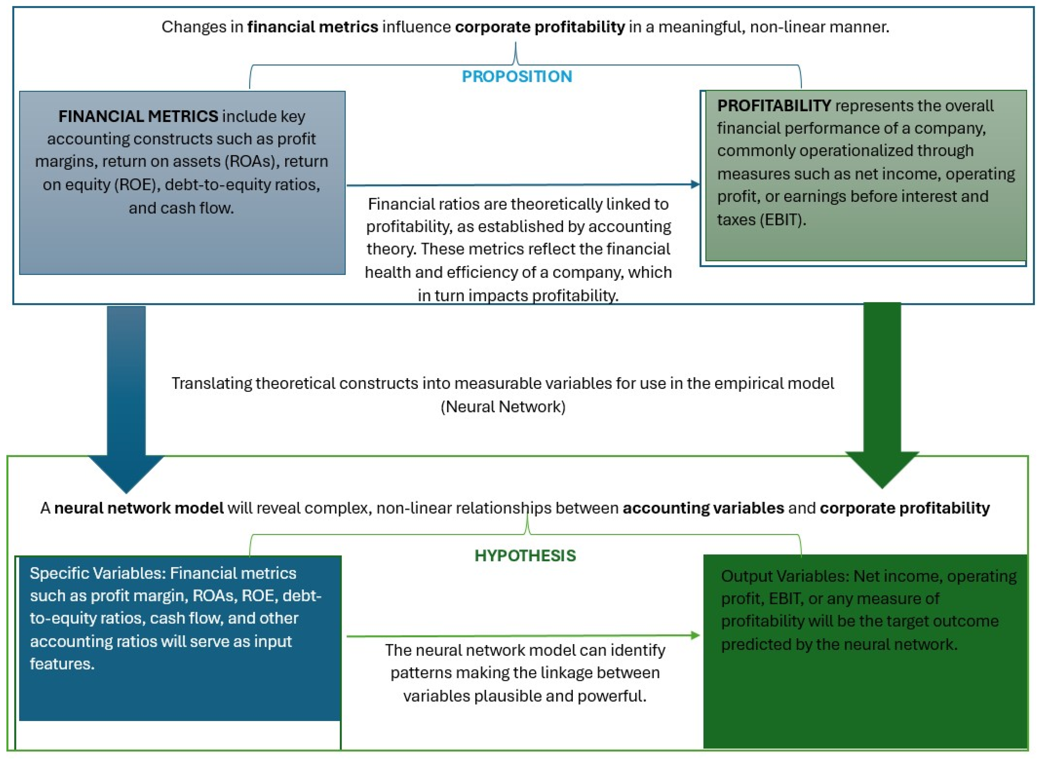
The most prominent variables in our study can be divided into two main categories as seen in Figure 1, namely input variables and output variables, each chosen to capture critical aspects of a company’s financial health and performance.

The input variables represent key financial metrics that have traditionally been linked to profitability and represent the key financial constructs that our neural network model uses to predict profitability, providing a different lens through which to view a company’s operational and financial efficiency.

On the output side, our primary output variable is profitability, which allows us to measure different dimensions of profitability, each relevant to various strategic decisions within the business. By analyzing the interaction between these input and output variables, our study aims to reveal patterns and insights that are crucial for financial forecasting and strategic decision making [8].

The integration of neural networks into accounting practices has garnered significant attention in recent years, reflecting a broader trend towards leveraging artificial intelligence for financial forecasting and decision making.

Various international studies, highlighting the theoretical foundations, practical applications, and socio-economic implications of employing neural networks in accounting, show that neural networks have been employed to predict financial metrics, such as earnings, cash flows, and stock prices. Their ability to learn from historical data enables them to provide forecasts that adapt to changing market conditions.

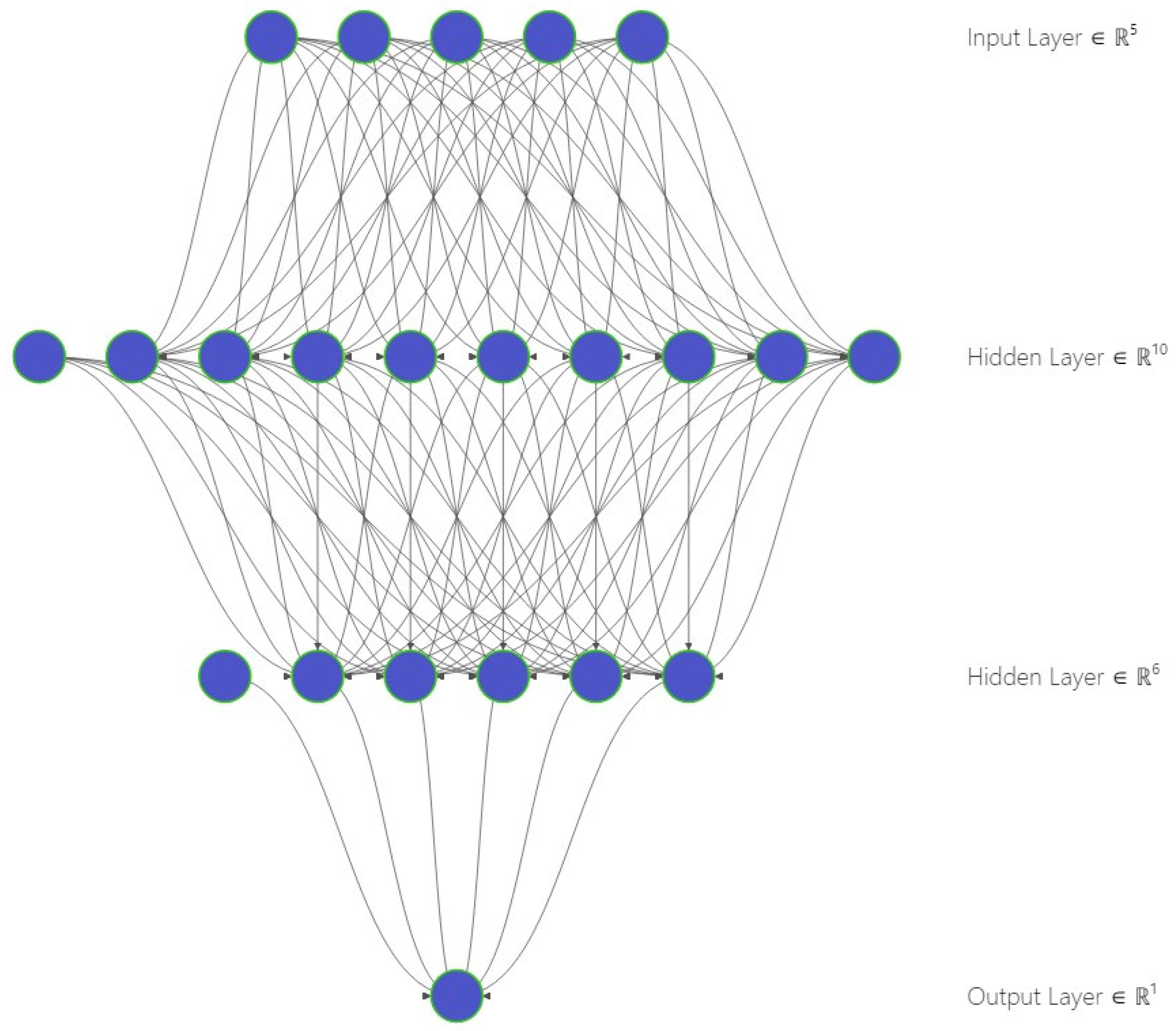
In accounting, we are constantly evaluating key financial indicators, like profit margins, return on assets, debt-to-equity ratios, and cash flow, that represent a company’s health, efficiency, and risk levels. When creating this neural network, all these metrics enter the model through the input layer, which has five nodes, one for each of these core metrics, and each node is like a doorway into the neural network, where we feed in financial signals [25].

Our neural network model is set up to accomplish this by incorporating pivotal accounting ratios and profit margins, like return on assets, return on equity, debt-to-equity ratios, and cash flow, according to which we can uncover complex interdependencies that traditional linear models tend to miss. We can express the architectural structure of our model using mathematical notation, where:

$$\mathrm{X}=\left[\begin{array}{cc}X1& X2\\ X3& X4\end{array}\right]=\left[\begin{array}{cc}ProfitMG& ROA\\ ROE& CashFlow\end{array}\right],$$

representing the multi-dimensional input layer, capturing a company’s “financial DNA”.

Each hidden layer refines the information, allowing the model to learn nonlinear interdependencies that simple linear regressions might overlook. For instance, partial derivatives of the output with respect to each pair of inputs can be nonzero, indicating that changes in the debt-to-equity ratio can alter how cash flow impacts profitability. This can capture real-world complexities, such as liquidity constraints exacerbating debt costs or synergy effects between efficient asset utilization and return on equity:

$${\displaystyle \frac{{\partial }^2\widehat{y}}{\partial x_i\partial xj}}\ne 0(\mathrm{for}\mathrm{some}\mathrm{i}\ne j)$$

The first hidden layer serves as a broad sweep of financial metrics, similar to a team of accountants each bringing a unique perspective on profitability factors, and allowing for the initial discovery of nuanced interactions, like the interplay of debt load and ROAs. Each node in the first hidden layer is like a miniature economic analysis that tries to find connections or correlations or trends or patterns among the five-input metrics. One node might learn how variations in the debt-to-equity ratio affect profitability in different cash flow scenarios, another might pick up on how the return on assets correlates with the return on equity over time, and so on and so forth, and can be expressed as follows:

Learned Weights and Bias

$${\mathit{W}}^{\left(1\right)}\in {\mathbb{R}}^{10\times 5}\mathrm{and}{b}^{\left(1\right)}\in {\mathbb{R}}^{10}$$

Nonlinear Transformation

$$h^{\left(1\right)}={\sigma }^{\left(1\right)}(W^{\left(1\right)}x+b^{\left(1\right)})=⌈\begin{array}{c}{h}_1\\ \dots \\ h_{10}\end{array}⌉$$

where ${\sigma }^{\left(1\right)}(.)$ is an activation function like the ReLU, tanh, or sigmoid.

The second hidden layer focuses on deeper relationships uncovered by the first layer that revealed how subtle variations in cash flow or asset returns might ripple through the company’s financial structure and distills the most salient patterns before the final prediction, taking the insights from layer one, like how various metrics interact, and rethinking them, thus combining them into more nuanced, second-level perspectives.

Learned Weights and Bias

$${\mathit{W}}^{\left(2\right)}\in {\mathbb{R}}^{10\times 6}\mathrm{and}{b}^{\left(2\right)}\in {\mathbb{R}}^6$$

Nonlinear Transformation

$$h^{\left(2\right)}={\sigma }^{\left(2\right)}(W^{\left(2\right)}h+b^{\left(2\right)})=⌈\begin{array}{c}{h}_1\\ \dots \\ h_6\end{array}⌉$$

The output layer aggregates the refined insights from the second hidden layer to predict overall profitability, reflecting the final metric of interest in strategic decision making.

Learned Weights and Bias

$${\mathit{W}}^{\left(3\right)}\in {\mathbb{R}}^6(\mathrm{or}{W}^{\left(3\right)}as1\times 6matrix)\mathrm{and}{b}^{\left(3\right)}\in {\mathbb{R}}^6$$

As well as the formula for profitability predictions:

$$\widehat{y}={\sigma }^{\left(3\right)}(w^{\left(3\right)}{h}^{\left(2\right)}+b^{\left(3\right)})$$

The input layer provides the model with the core ingredients it needs to understand a company’s financial DNA.

Our motivation for this design is to balance model complexity and interpretability in line with longstanding practice in regard to neural network architecture and to reflect on the nuanced reality of financial data arising from different regulatory frameworks, such as the IFRS and US GAAP.

A strictly minimal architecture might overlook these cross-standard interactions and misrepresent relationships that only emerge when processing the data during intermediate stages, because a single hidden layer might not capture the variety of subtle, nonlinear relationships we encounter in modern financial metrics. Even something as fundamental as net income can be reported differently across regions, especially when companies adhere to distinct accounting standards [26].

Our two-layer approach reflects a compromise between these extremes. Empirically, we have seen that one hidden layer may be insufficient to tease out the layered intricacies in financial statements [27], for instance, the interplay between standardized elements like revenue recognition policies in the IFRS and more nuanced items like stock-based compensation under the US GAAP. By devoting one layer to learning universal patterns, such as fundamental ratios or cash flow structure, and a second layer to refining those representations, we can better adapt to varying disclosures and classification practices. While this is not an entirely novel insight, two-layer networks are well-documented in the literature, the design choice remains meaningful for corporate accounting data, which rarely conform to a single, uniform standard [26].

We have two hidden layers in this network, with 10 nodes in the first and 6 nodes in the second. Each hidden layer analyzes and reanalyzes the financial metrics, refining, and combining them in new ways. In the first hidden layer, we start with a broader, more comprehensive sweep across the data similar to a group of skilled auditors, each taking a different slice of the financials, identifying the relationships and nuances in regard to each metric, because it is one thing to know a company’s profit margin and another to understand how that margin interacts with debt levels or asset efficiency. This first layer, with 10 nodes, allows us to start seeing these nonlinear relationships. The second hidden layer, with six nodes, focuses on understanding how subtle changes in cash flow, for example, or asset returns, can ripple out across the business’s entire profitability picture and lead to deeper insights, zeroing in on what really impacts profitability.

The output layer has a single node dedicated to profitability prediction, based on what is observed in the financial metrics.

In Figure 2, we outlined our proposed architecture to build a clear theoretical network framework, using the NN-SVG to explain each layer’s purpose [23], how it corresponds to the accounting variables, and why this specific structure was chosen. The next step is to set up a similar architecture in the TensorFlow Playground to experiment with different learning dynamics, adding a practical dimension to the theoretical framework. The TensorFlow Playground shows visualizations of how well the network’s predictions match the data distribution. If the pattern aligns closely with the data, the model is learning effectively.

First, we start with a dataset that is input into the TensorFlow Playground, which represents simple data patterns, choosing the plane dataset to approximate a regression problem like predicting profitability. In our model, the plane dataset is made up of the profit margin, return on assets (ROAs), return on equity (ROE), debt-to-equity ratio, and cash flow. These metrics feed into the network to help predict the target like, for example, net income or EBIT (earnings before interest and taxes). For this to function, we also must set the ratio of training to test data.

The ratio of training to test data represents the historical accounting records that teach the network patterns and test data that act as new records that challenge the network to make accurate predictions. In this case, we set it up as 70% for training and 30% for testing, allowing the model to learn effectively from past data and then evaluate its predictive power on fresh, unseen data. We started with zero noise to keep things simple, but, in a full model, adding noise helps make the network robust, able to handle real-world variability through adding randomness to the data, simulating unpredictable fluctuations, like economic events or market volatility, that introduce uncertainty.

In the TensorFlow Playground, we have options to include X1, X2, X1², X2², X1X2, sin(X1), and sin(X2), which represent various data transformations. In our case, X1 and X2 represent simple financial metrics like the ROAs and profit margin, and X1² and X2² are used to capture the nonlinear relationships of the ROAs and profit margin to profitability.

The hidden layers are the core of the accounting neural network. Each layer represents a stage in the decision-making process, much like an accountant analyzing data, layer by layer. In a real-world financial model, more nodes and layers might be necessary, but this simplified structure helped us to grasp the basics. Each layer has an activation function, and we chose the ReLU (Rectified Linear Unit), helping the network to handle nonlinear data that can curve, peak, and plateau. Use of the ReLU helps us to make sense of complex patterns and understand that, for example, the ROAs does not increase net income endlessly and there are diminishing returns. For our accounting neural network, the learning rate is crucial for the speed at which AI learns from new data, and we set it to 0.03, while keeping the batch size at 10, making learning efficient, while allowing the model to adjust gradually. If we set a higher value, the model might learn too quickly without depth, but if we set it too low, the model learns too slowly. For our financial model, we believe a learning rate of 0.001 to 0.01 is acceptable for balancing accuracy and efficiency. We also must be careful to prevent the network from focusing too closely on one year’s data trends and failing to generalize for future years. Because ours is a theoretical model, we did not set up regularization to keep things simple, but in a full model, we suggest using Dropout (randomly ignoring nodes) or L2 Regularization (penalizing large weights) to ensure the network generalizes well.

Based on the input data, as shown in Figure 3, we started with a test loss of 0.808 and a training loss of 0.840, letting the model train for at least 50 epochs initially, while observing how both the test loss and training loss change. For most models, if both losses stabilize within a low range after 100–200 epochs, this is often a good place to stop [22].

After 50 epochs, both the test loss and training loss were at exactly 0.000, indicating a red flag in neural network training, indicating overfitting. Our model has overfit the data, indicating that our model has learned to predict the training data perfectly, which is unusual in real-world applications and suggests it has “memorized” the data rather than learning generalizable patterns. At the same time, a test loss of 0.000 suggests that the model is also perfectly predicting the test set due to a lack of complexity in the data or having excessive capacity, like too many nodes/parameters, relative to the complexity of the financial data.

In our financial forecasting and most real-world accounting applications, achieving a perfect fit in regard to both the training and test data is unrealistic, because real financial data tends to be noisy and complex.

To counter overfitting, we applied some adjustments. We increased the regularization rate to 10, preventing overfitting by adding a penalty for overly complex models, we reduced the number of nodes in the hidden layers from eight layers to six layers and from four additional layer to 2 layers, respectively, and we also increased the amount of noise to a value of 10 to increase the dataset’s complexity.

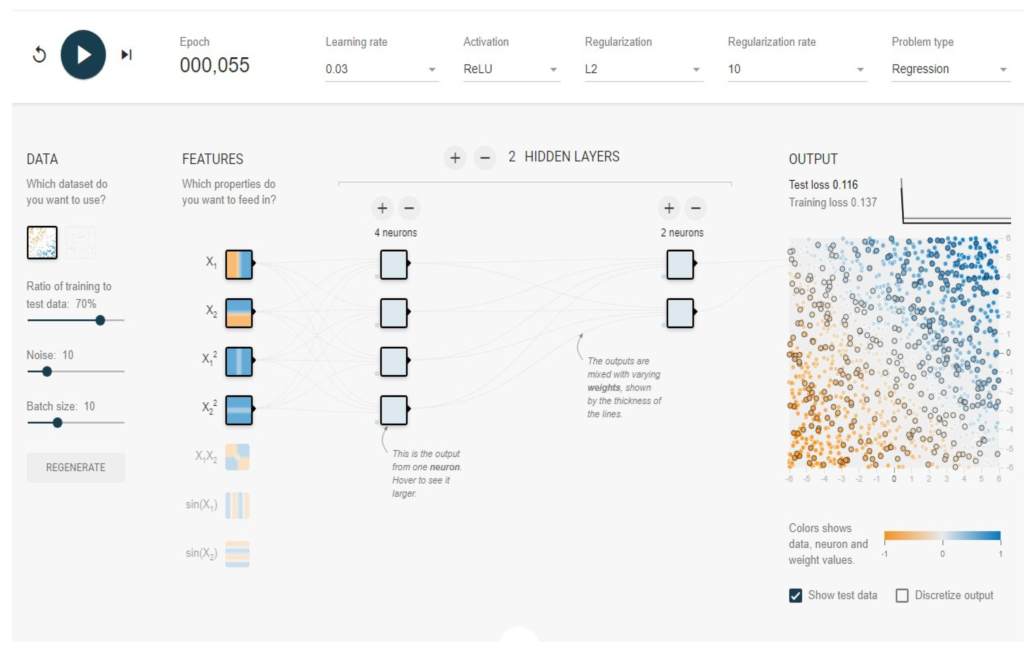
Regarding this setup, we let it run to about 50 epochs to see whether the losses stabilized, and then we interpreted the results based on the final values and behavior of the losses. The new setup can be seen in Figure 4, starting with a test loss of 0.272 and a training loss of 0.316.

Based on the new input data, we started with a test loss of 0.272 and a training loss of 0.316, letting the model train for at least 50 epochs initially, while again observing how both the test loss and training loss changed [24].

With the test loss and training loss at 0.116 and 0.137, respectively, the model is no longer showing signs of extreme overfitting. These losses are low and close to each other, which suggests that the model has learned generalizable patterns rather than just memorizing the training data and introducing regularizations, and the introduction of noise likely helped the model become more robust, enabling it to handle variability in the data better.

As presented in Figure 5, starting at a test loss of 0.272 and a training loss of 0.316 and ending with a test loss of 0.116 and a training loss of 0.137 shows steady progress in regard to learning. This gradual reduction in losses over 55 epochs indicates that the model is effectively learning from the data and converging without overfitting, and is now better suited to predicting financial metrics, as it is more likely to generalize well to new data, which is crucial in real-world financial forecasting.

To ensure a more stable outcome, we ran a few more epochs to confirm its stability and ensure the losses did not start diverging. After an additional 25 epochs, the test loss was 0.116 and the training loss was 0.137, suggesting optimal parameters.

The next logical step would be to train our network and test it with new unseen data, confirming that our model can generalize well beyond the initial sample, but this being a theoretical model we stopped here.

Given our current results, we concluded that the model has strong stability and convergence. Both losses have reached a steady point, low and close to each other, which is a great indicator of effective learning, revealing that the model has picked up on real patterns in the data without overfitting to the specifics of the training set and finding a balance that is likely to make it reliable for future predictions based on similar data.

The robustness and regularization adjustments, adding a bit of noise, and reducing the complexity of the hidden layers resulted in visible improvements, showing us that the model can handle the kind of variability we expect in real-world financial data and that it was not just memorizing details, but understanding broader trends that will make it adaptable in practical applications.

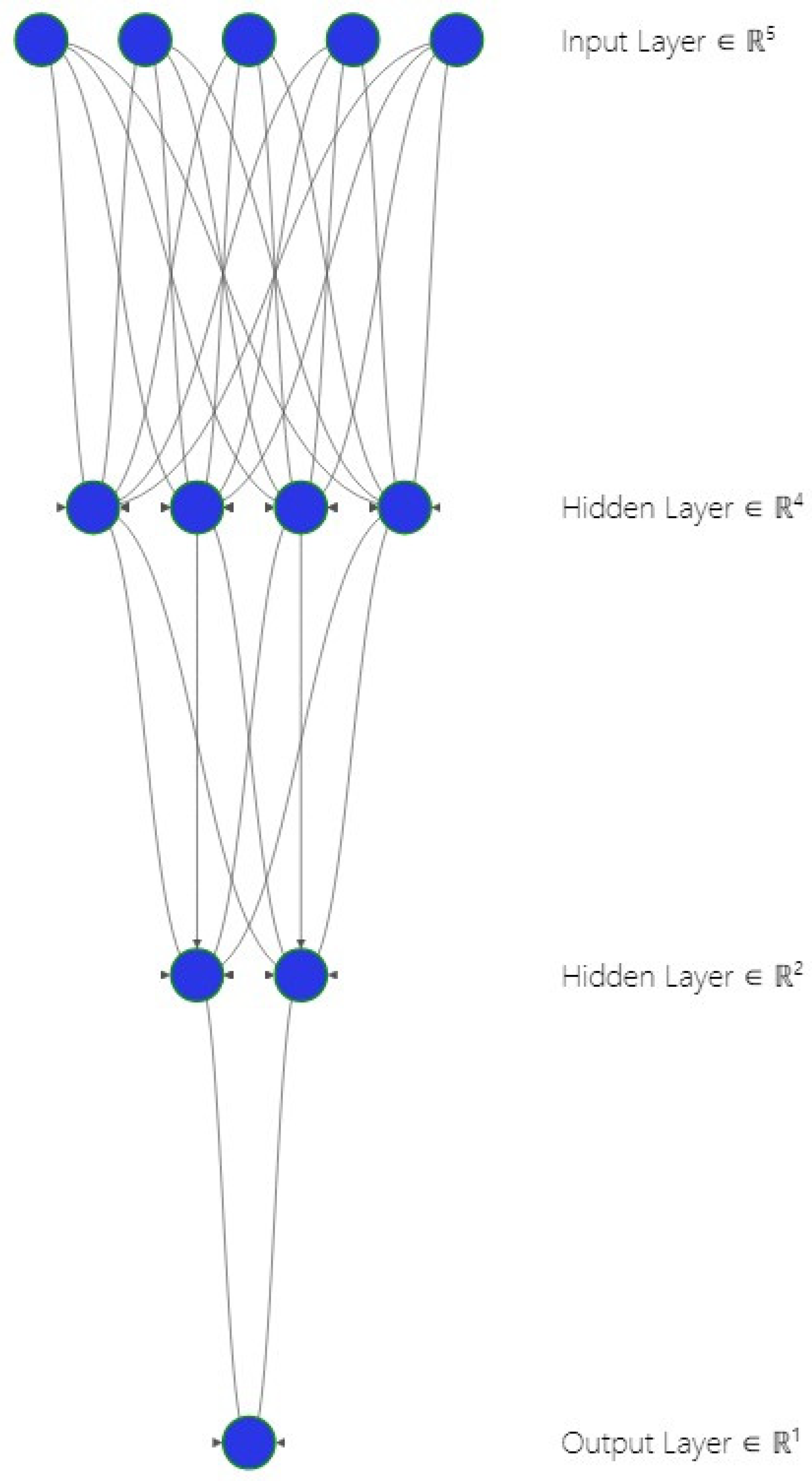
Based on our findings, we redesigned the neural network diagram, using the NN-SVG, to reflect our findings in the TensorFlow Playground. The new conceptual diagram for our accounting neural network is presented in Figure 6.

Adapting the new conceptual NN-SVG diagram, we can state that the new structure 4–2–1 is better aligned with our empirical findings in the TensorFlow Playground that include improved generalization and reduced overfitting when dealing with real-world financial data.

We can express the new architectural structure of out model using a mathematical notation, where:

$$\mathrm{X}=\left[\begin{array}{cc}X1& X2\\ X3& X4\end{array}\right]=\left[\begin{array}{cc}ProfitMG& ROA\\ ROE& CashFlow\end{array}\right],$$

by using fewer nodes (four in the first layer, two in the second), the model is less prone to overfitting based on smaller datasets and is easier to regularize.

As with the previous model, any second derivative of the output with respect to two different inputs can be nonzero, indicating that changes in one metric can amplify or dampen the influence of another on overall profitability:

$${\displaystyle \frac{{\partial }^2\widehat{y}}{\partial x_i\partial xj}}\ne 0(\mathrm{for}\mathrm{some}\mathrm{i}\ne j)$$

The first hidden layer captures general relationships among key accounting ratios and begins to reveal the relationships and nonlinear interactions among the five key accounting metrics.

Learned Weights and Bias

${\mathit{W}}^{\left(1\right)}\in {\mathbb{R}}^{4\times 5}$ is the weight matrix, and $b^{\left(1\right)}\in {\mathbb{R}}^4$ is the bias vector.

Nonlinear Transformation

$$h^{\left(1\right)}={\sigma }^{\left(1\right)}(W^{\left(1\right)}x+b^{\left(1\right)})=⌈\begin{array}{c}{h}_1\\ h\dots \\ h_4\end{array}⌉$$

where ${\sigma }^{\left(1\right)}(.)$ is an activation function like the ReLU, tanh, or sigmoid.

The second hidden layer focuses on subtler variations, when changes in cash flow or asset performance might ripple through the firm’s overall profitability dynamics.

Learned Weights and Bias

${\mathit{W}}^{\left(2\right)}\in {\mathbb{R}}^{2\times 4}$ is the weight matrix, and $b^{\left(2\right)}\in {\mathbb{R}}^2$ is the bias vector.

Nonlinear Transformation

$$h^{\left(2\right)}={\sigma }^{\left(2\right)}(W^{\left(2\right)}h+b^{\left(2\right)})=⌈\begin{array}{c}{h}_1\\ h_2\end{array}⌉$$

The output layer aggregates the refined insights from the second hidden layer to predict overall profitability and has just one node:

Learned Weights and Bias

${\mathit{W}}^{\left(3\right)}\in {\mathbb{R}}^2$ (or $W^{\left(3\right)} as 1 \times 2 matrix$) and $b^{\left(3\right)}\in \mathbb{R}$.

As well as the formula for profitability predictions:

$$\widehat{y}={\sigma }^{\left(3\right)}(w^{\left(3\right)}{h}^{\left(2\right)}+b^{\left(3\right)})$$

where $\widehat{y}$ is the single output node predicting profitability, and, depending on whether we expect positive/negative or unbounded values, ${\sigma }^{\left(3\right)}$ might be linear or nonlinear.

Regarding the theoretical model’s predictive performance, we see acceptable outputs for a forecasting model in finance. With a test loss of around 0.116 and a training loss close behind at 0.137, we achieve a level of accuracy that provides a solid basis for reliable insights. In accounting, we know perfect predictions are rare, but this model’s performance provides us with a strong foundation for making meaningful, data-driven forecasts.

The effectiveness of this model hinges on the quality and representativeness of the financial data used and, without a clear understanding of the data sources, it is challenging to assess whether the model generalizes well across different industries, economic conditions, and timeframes. Also, the financial metrics selected, such as profit margin, ROAs, and debt-to-equity ratio, should also be justified as the most relevant for forecasting profitability, ensuring they offer consistent value across varied financial scenarios.

Of course, interpretability is another critical area of concern for us in terms of the empirical development of the theoretical model. Neural networks in the accounting field can have limited usefulness for strategic decision making, and the choices made regarding the regularization rate, noise levels, and hidden layer complexity need careful justification. While regularization and noise were introduced into our theoretical model proposal to improve its robustness, it is essential for future real-life scenarios to know whether these adjustments were systematically validated or whether they were based on empirical evidence from validation data.

To ensure that these findings can be validated beyond just one training set, we incorporated a form of cross-validation, even though we are dealing with synthetic data. We rotate different parts of the dataset in and out of the training and testing phase, so that every input is analyzed, reducing the chance that the projection of a robust model can be generated when, in fact, it might only excel based on one subset of observations.

One straightforward way to gauge how much the predicted values deviate from the true outcomes is to compute error metrics that summarize the differences across all the data points measuring the average of the squared differences between the predicted and actual values to heavily penalize larger errors, since the differences are squared. Equally important is the interpretation of these metrics in the context of accounting and finance. A tiny difference in the mean squared error between two models might, in practical terms, translate into a huge disparity in profit forecasts. Through the use of our theoretical framework, we must suggest and incorporate in future empirical real-life models, not just the numerical performance measures, but also how they translate in regard to decisions made, and whether a company might decide to alter its capital structure or allocate resources differently based on our model’s profitability predictions. By linking those statistical figures back to strategic accounting implications, we can install a richness into the empirical model that pure numbers alone cannot convey.

Traditional models often fall short when the data is highly interconnected and do not follow predictable patterns. But with neural networks, we can dig deeper, finding patterns that would otherwise go unnoticed and delivering forecasts that hold up in the real world [22,23].

While our research presents a theoretical framework and proof of concept using synthetic data, we recognize the importance of demonstrating real-world applicability and, by incorporating empirical steps, we aim to strengthen the credibility and applicability of the proposed neural network framework.

We introduced a targeted empirical exercise to assess the practical viability of our neural network framework, retrieving a publicly available dataset from Kaggle, containing financial indicators for S&P 500 companies as seen in Figure 7, such as price, earnings per share (EPS), and market capitalization, and used MATLAB2024b to predict each firm’s share price, using actual financial data in MATLAB2024b to see whether our neural network could indeed capture the real dynamics that underlie corporate metrics. Our intention was to see how these fundamental inputs might predict a company’s share price, thereby giving us a first taste of how well our model’s architecture translates to the real world, because raw data almost always comes with missing fields, outliers, and uneven distributions.

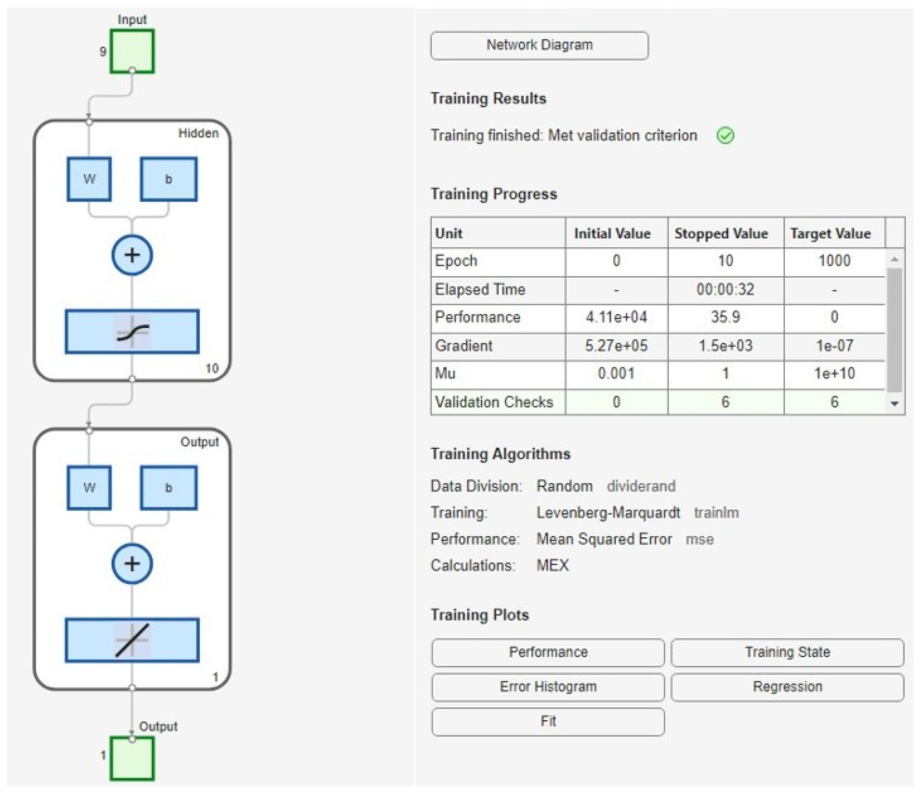
Using the Deep Learning Toolbox R2024b, once we had a reliable subset, we fed it into MATLAB, split the data into a training portion and a smaller test portion, and then applied a modest, single-hidden-layer neural network.

Figure 8 illustrates that our neural architecture could learn meaningful relationships from real figures, without relying exclusively on synthetic distributions or curated test settings, and the empirical text reveals that even this minimal model captured noticeable patterns in pricing, albeit with the sort of error margin one would expect when using only a handful of basic metrics to predict something as complex as share price.

After cleaning and preprocessing the data, we employed an 80/20 train–test split, using a single-hidden-layer neural network to capture potential nonlinear relationships among variables like the P/E ratio, dividend yield, and EBITDA. Our aim was not to create a production-grade forecasting system, but rather to showcase that the proposed architecture indeed learns meaningful patterns from real-world financial data. We then measured its performance via the mean squared error (MSE) and root mean squared error (RMSE). In terms of our test set, the model demonstrated an RMSE of approximately 32.48, suggesting a moderate level of predictive accuracy for a first pass. While certain outliers and sector-specific nuances inevitably reduced the precision, this finding indicates that even a lean implementation of our proposed framework can extract informative signals from fundamental stock data.

We acknowledge that share prices hinge on far more than a handful of numerical ratios, with market sentiment, macroeconomic shifts, and competitive landscapes all playing substantial roles. Yet, the results demonstrate that our theoretical model can be adapted to real-world data, validating its core premise. For a future, more robust iteration, we plan to expand the feature space and refine the neural network hyperparameters, aiming for an even tighter fit.

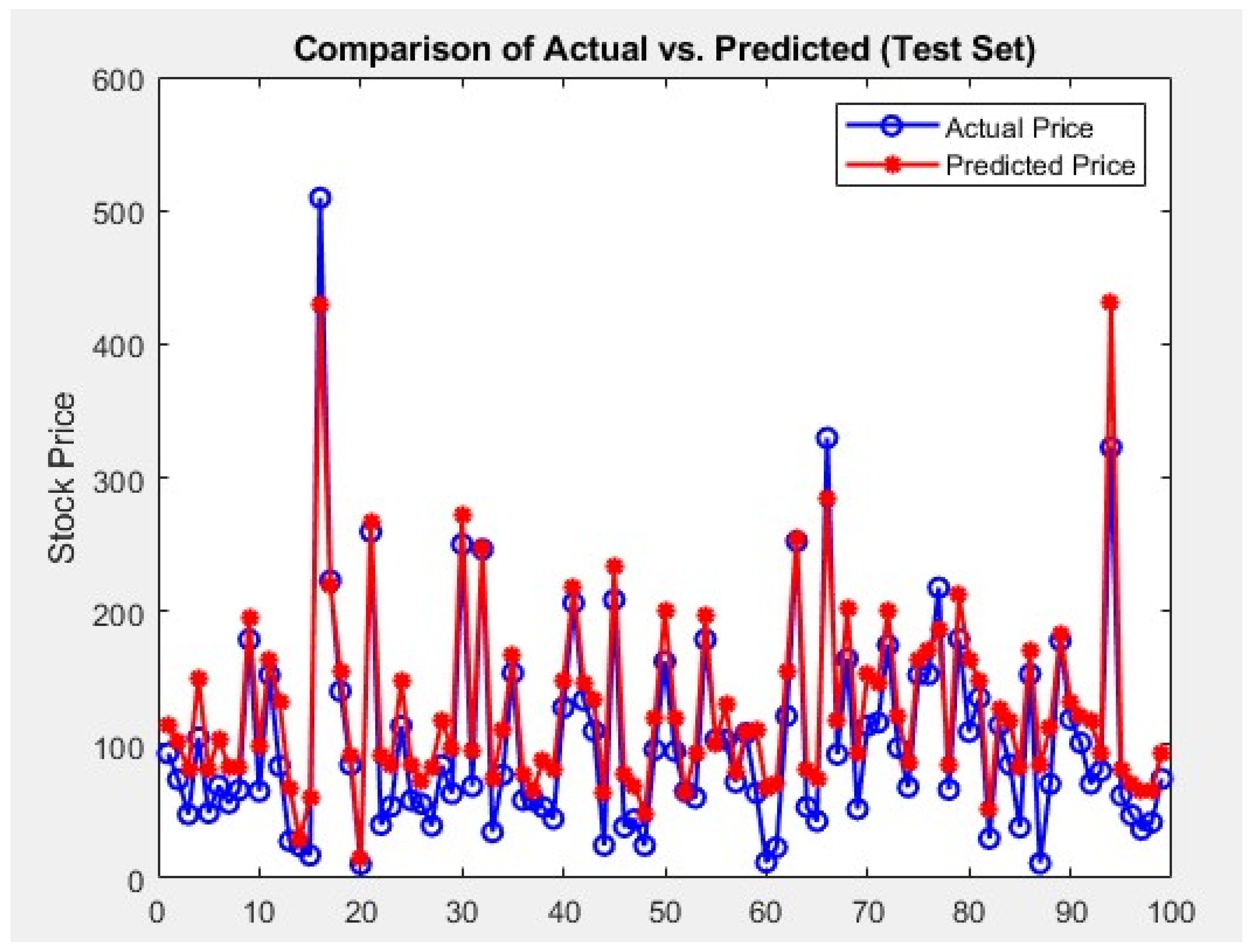
The final model obtained an MSE of 1054.68 and an RMSE of 32.48 based on the test set, implying an average deviation of about 32 USD from the actual stock price. Figure 8 compares actual vs. predicted prices, given that several stocks in our sample have prices ranging from 50 USD to more than 300 USD, an average deviation of 32 USD is a good starting point, but can likely be improved with more features and/or hyperparameter tuning.

Figure 9 shows that, while the predicted prices generally track the actual prices, there is noticeable divergence in regard to certain samples. This indicates that the network captures some core relationships, but lacks complete accuracy, likely due to omitted factors, such as market sentiment or macroeconomic data.

Because of the potential impact of this model on strategic financial decisions, ethical and regulatory considerations must be addressed. Predictive models in accounting carry significant responsibility, as they influence key decisions that affect various stakeholders [28]. Thus, any concerns around transparency, accountability, and the responsible use of AI in financial forecasting should be directly addressed to ensure the model supports informed, ethical decision making [21].

5. Conclusions

Combining fundamental accounting principles with a neural network, we are creating a model that does not just analyze financial data, but learns from it, transforming traditional financial forecasting into something dynamic, insightful, and incredibly relevant to today’s fast-moving financial world.

NN-SVG allows you to design custom network architectures visually, showing the exact number of layers, nodes, and connections in a clear, static diagram. This can be extremely helpful for laying out the architecture you want to explain conceptually, especially in papers, presentations, or documentation. The TensorFlow Playground, on the other hand, offers a dynamic, interactive environment, which allows you to see how a neural network learns from the data in real time. It is limited in terms of customizability in regard to the node counts and layer depth, but it is great for seeing how training affects the model over epochs, and how changing the hyperparameters, like the learning rate or regularization, impacts the results. Combining NN-SVG with the TensorFlow Playground is a strong approach for theoretical explorations, as each tool contributes unique value to a cohesive framework that is both clear in structure and practical in terms of the insight gained.

Despite these limitations, our results produced using MATLAB show that neural networks can provide a baseline level of predictive insight into stock prices using fundamental ratios. This empirical test demonstrates the real-world feasibility of our theoretical model. Running this exercise in MATLAB confirmed that our neural network can handle real accounting inputs without crumbling under the messiness of the real world. We have seen that financially relevant inputs like profit margins, cash flow, or price-to-earnings ratios retain enough informational strength to guide a modest neural network toward sensible predictions, even when faced with the inherent noise of real-world figures. By introducing the S&P 500 dataset into our research, we tried to underline that our theoretical model scales beyond controlled, synthetic distributions and can be a base for more unpredictable circumstances. The resulting forecasts are still at an early stage and, absolute precision can hardly be expected when dealing with the nuances of markets and firm-level variations, but they exemplify a sound step forward.

In regard to future developments of the neural network suggested in this research, it would be beneficial to consider alternatives, like R-squared, that might offer more insight into how well the model performs.

Using neural networks in accounting is not just about proving that neural networks can work in accounting and finance, it is about showing how technology can empower us to make smarter, data-driven decisions.

Future research will establish a clear performance benchmark that will be vital to fully contextualize our results. In future revisions, we plan to include comparisons with widely used techniques, such as linear regressions, tree-based ensembles, or other neural architectures, to demonstrate how our network’s performance measures up against existing standards. This addition will help clarify where our model offers significant advantages and where further refinements might be beneficial.