Article

Research on Distributed Optimization Scheduling and Its Boundaries in Virtual Power Plants

School of Electrical Engineering, Xinjiang University, Urumqi 830046, China
*
Author to whom correspondence should be addressed.
Electronics 2025, 14(5), 932; https://doi.org/10.3390/electronics14050932
Submission received: 29 January 2025 / Revised: 20 February 2025 / Accepted: 25 February 2025 / Published: 26 February 2025
(This article belongs to the Special Issue Planning, Scheduling and Control of Grids with Renewables)

Abstract

:
To improve the operational efficiency of the Virtual Power Plant (VPP) and the effectiveness and reliability of scheduling boundary characterization, this paper proposes a time-decoupled distributed optimization algorithm. First, based on the Lyapunov optimization theory, time decoupling is implemented within the VPP, transforming long-term optimization problems into single-period optimization problems, thereby reducing optimization complexity and improving operational efficiency. Second, the Alternating Direction Method of Multipliers (ADMM) framework is used to decompose the optimization problem into multiple subproblems, combined with a hybrid strategy to improve the particle swarm optimization algorithm for solving the problem, thus achieving distributed optimization for the VPP. Finally, to facilitate intra-day interaction between the VPP and the distribution network, the remaining controllable capacity of the VPP’s devices is used as the spinning reserve to address renewable energy fluctuations. A dynamic scheduling boundary model is constructed by introducing wind and solar fluctuation factors. Based on time decoupling and algorithm improvement, the scheduling boundaries are solved and updated on a rolling basis. Simulation results show that, firstly, the time decoupling strategy based on Lyapunov optimization has an error of less than 3%, and the solving time is reduced by 86.11% after decoupling, significantly improving solving efficiency and validating the feasibility and effectiveness of the time decoupling strategy. Secondly, the hybrid strategy-improved particle swarm optimization algorithm achieves improvements in convergence speed and accuracy compared to other algorithms. Finally, the VPP scheduling boundary and scheduling cost characterization times are 115 s and 6.7 s, respectively, effectively meeting the timeliness of VPP and distribution network interaction while ensuring the safety and reliability of the scheduling boundaries.

1. Introduction

The VPP, by aggregating the regulatory capacities of distributed energy resources, can effectively compensate for the insufficient regulation capabilities of renewable energy, providing a viable pathway for active participation in distribution network scheduling [1,2,3]. While the VPP shares certain external characteristics with traditional power plants, its internal operation and control mechanisms differ fundamentally. It must collaborate with distributed energy resources to respond to scheduling instructions from the higher-level grid under rapidly changing operational conditions, while ensuring the VPP remains in an economically and securely stable state. Therefore, studying the internal optimization scheduling of the VPP is essential for its participation in the scheduling of the main grid [4,5,6].
Currently, most studies on the internal optimization scheduling of VPP employ either centralized or distributed optimization methods. In terms of centralized optimization, Reference [7] proposed a bi-level optimization model for user demand scheduling based on virtual power source management, and solved it using an improved harmony search algorithm. The results showed that the improved method increased computational efficiency by 20.25%. Reference [8] established a stepwise carbon trading model to constrain system carbon emissions and formulated an optimization model to minimize operational costs and emissions. The model was solved using a particle swarm optimization algorithm with linearly decreasing constraints. Simulation results indicated that the improved particle swarm algorithm reduced the operation time by 7%, respectively. Centralized optimization methods can comprehensively consider the system’s state, making them suitable for small-scale problems and providing high accuracy. However, as the problem size increases, computation time and memory consumption increase sharply, leading to a significant decrease in efficiency. In contrast, distributed optimization decomposes the problem into local sub-problems, significantly improving computational efficiency and scalability in large-scale systems [9,10,11]. Reference [12] utilizes a distributed optimization method to achieve the coordinated operation of the VPP and conventional units, and compares it with centralized optimization. The cost error is only 1.54%, while the computational efficiency is significantly improved. Reference [13] proposes a distributed active power and reactive power optimization control method for active distribution networks, which converges after only 62 iterations. However, the robustness and convergence of the above methods are often not as good as the ADMM algorithm.
ADMM, as a classical distributed optimization algorithm, has been widely applied to the solution of optimization problems. Reference [14] proposed an ADMM algorithm with parallel regularization for solving the operational costs of campus clusters. Simulation results showed that the median differences in operational costs obtained by the conventional ADMM algorithm and the improved ADMM algorithm were 0.25%, 0.54%, 0.24%, and 0.19%, respectively. The improved ADMM algorithm significantly reduced the solution time for each iteration while ensuring the accuracy of the results. References [15,16] demonstrate the effectiveness of the ADMM algorithm in energy systems but note that some accuracy may be sacrificed when decomposing optimization problems. Additionally, the power regulation of energy storage devices within the VPP exhibits temporal coupling, which significantly affects the computational efficiency of solving the full-period optimization problem. References [17,18] use temporal decoupling to decompose the optimization problem into 24 periods for sequential solving, thereby transforming multi-period optimization into single-period optimization. Reference [19] relaxes the internal coupling constraints of the solving model and decouples them into a virtual queue stability problem using Lyapunov optimization. Reference [20] designs an energy router port coordination control algorithm based on the Lyapunov optimization method, forming an energy management strategy for an energy hub that includes energy routers. However, these methods do not quantitatively analyze the impact of temporal decoupling on optimality.
In recent years, data-driven modeling methods based on machine learning have been widely applied in the power sector. Reference [21] uses data-driven techniques to construct models for the feasibility of dispatch instructions and interaction costs, significantly reducing optimization computation time while ensuring the internal information security of the virtual power plant. Reference [22] proposes a data-driven virtual power plant scheduling characteristic encapsulation modeling method, offering a new perspective for power system modeling. However, these methods still have some limitations. First, reinforcement learning models lack sufficient interpretability, leading to a lack of transparency in the decision-making process. Second, reinforcement learning requires large amounts of historical data for training, and the training process is time-consuming and requires real-time model updates, which increases the system’s computational burden and affects the feasibility of the application.
In addition, as a commercial entity, the VPP needs to interact actively with the distribution network to earn profits and ensure sustainable operation. Due to market competition, VPP operators are unwilling to disclose their internal models, which means that the VPP cannot be as easily understood by the distribution network regarding its real-time scheduling margin, unlike traditional power plants. When the distribution network has additional scheduling demands during the day, the dispatch center tends to interact more with traditional power plants to ensure grid security and power supply reliability. Nevertheless, VPP operators may promote market competition and enhance efficiency by disclosing partial data, for example, by using a “recruitment-participation” approach to attract more virtual power plants to participate, as shown in references [23,24]. However, the ultimate goal remains to improve overall efficiency through market competition. Therefore, VPPs need to report their scheduling boundaries to the distribution network, which, based on these boundaries and its own scheduling needs, issues dispatch instructions to the VPP. In this way, the VPP does not need to provide detailed physical models but can still allow the distribution network to understand its scheduling potential, which not only protects user data privacy but also improves utilization and economic efficiency.
There has been extensive research on the methods for characterizing the scheduling boundary of VPPs. Reference [25] generates multiple operating states using the Monte Carlo method and calculates the VPP scheduling for each state, using their collective results as the scheduling boundary of the VPP. Reference [26] applies the Gauss elimination method and Fourier–Motzkin elimination method to handle the equality and inequality constraints of the distribution network, mapping the operating space to the VPP gateway nodes. The aforementioned methods, however, do not consider the volatility and intermittency of renewable energy generation. Subsequently, some scholars have characterized the scheduling boundary by analyzing the probability density function of renewable energy output. Reference [27] randomly generates multiple scenarios based on the probability distribution functions of renewable energy and load fluctuations, and determines the scheduling boundary that satisfies all scenarios through optimization. Reference [28] considers the uncertainty of renewable energy using chance constraints, and at different confidence levels, transforms the chance constraints into deterministic constraints using percentiles, to solve for the scheduling boundary. The scheduling boundaries characterized by the aforementioned methods are based on a certain confidence level. Additionally, by utilizing the probability density function of renewable energy output combined with the Monte Carlo approach, the scheduling boundaries of the VPP under different states need to be calculated. This results in a heavy computational burden and makes it difficult to meet the timeliness requirements for intraday interaction between the VPP and the distribution network. Therefore, the ability to efficiently and reliably characterize the VPP scheduling boundary is a core issue for its participation in the distribution network scheduling [29,30,31].
Based on the aforementioned research findings and the issues that need to be addressed, the main contributions and innovations of this paper are as follows:
(1)
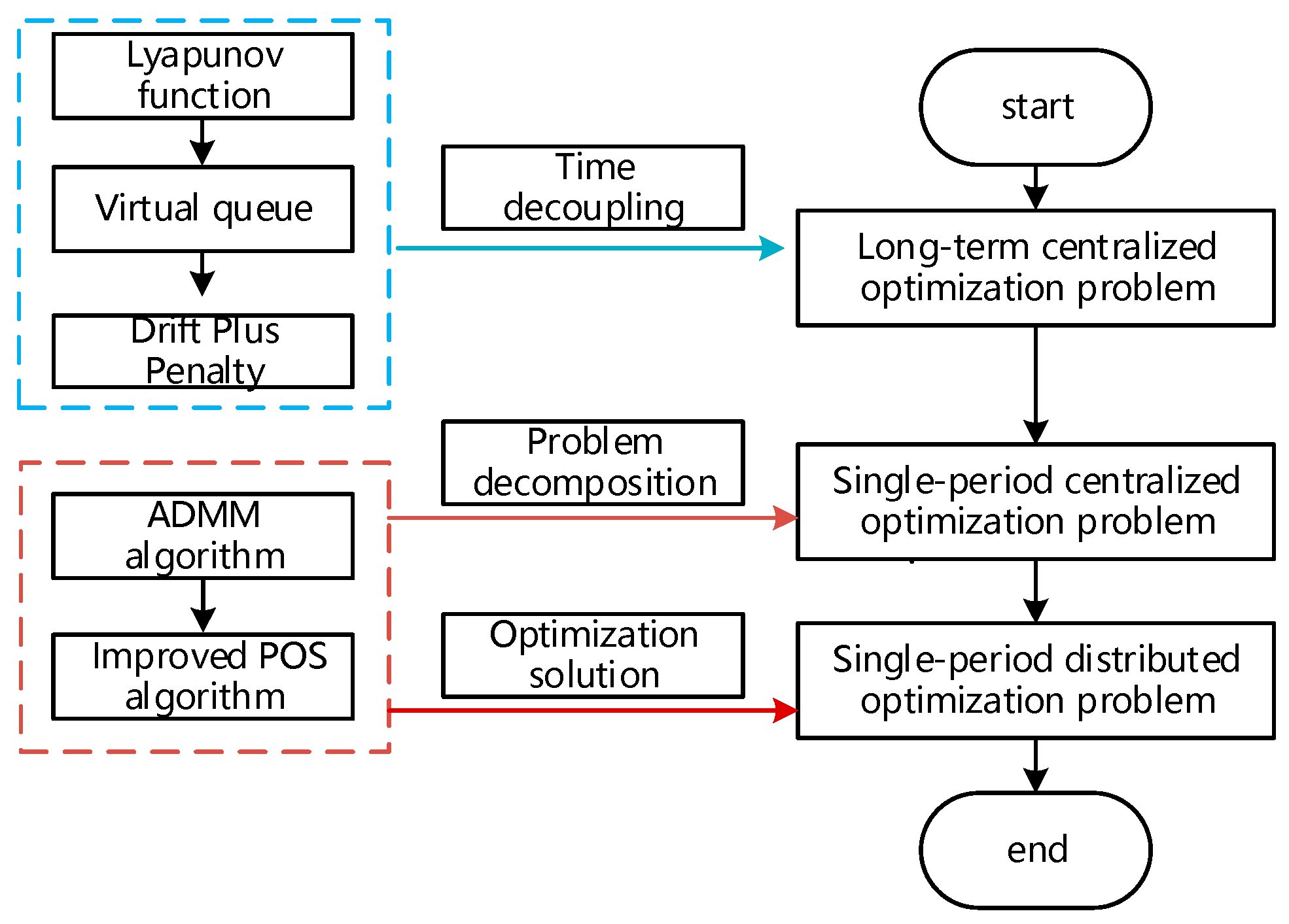
This paper proposes a time decoupling strategy based on Lyapunov optimization, which transforms the long-term optimization problem within the virtual power plant into multiple independent single-period optimization problems. This strategy significantly improves solution efficiency and has been validated for its feasibility and effectiveness in virtual power plants.
(2)
This paper adopts an ADMM distributed optimization framework, which further decomposes the single-period optimization problem into multiple subproblems. It is solved using a hybrid strategy-improved particle swarm optimization algorithm. This method not only enhances computational accuracy but also significantly increases solving speed.
(3)
A dynamic scheduling boundary model is constructed by utilizing the remaining adjustment capacity of the virtual power plant’s controllable devices. Based on this and combined with the time decoupling strategy and algorithm improvements, efficient, reliable characterization and rolling updates of the scheduling boundary are achieved, thereby effectively promoting the interaction between the virtual power plant and the distribution network.
Brief introduction to the structure of the paper:
Section 1: Introduction to the current challenges in VPP optimization scheduling and the characterization of scheduling boundaries.
Section 2: Introduces the composition, operational strategy, and scheduling process of the VPP, and analyzes the mathematical models of each unit within the system.
Section 3: Analyze the time-coupling constraints within the virtual power plant and propose a time decoupling method based on Lyapunov optimization. A distributed optimization framework based on ADMM is designed, and an improved solution to the issues of the particle swarm optimization algorithm is proposed.
Section 4: Analyzes the virtual power plant scheduling instructions and proposes a method for characterizing the VPP scheduling boundary based on spinning reserve.
Section 5: Through case studies, the feasibility of the time decoupling strategy in virtual power plants and the effectiveness of the algorithm improvements were validated. In addition, the VPP scheduling boundary was characterized and a comparative analysis was conducted.
Section 6: Summarizes the main contributions of the paper, discusses the limitations of the research, and outlines directions for future studies.

2. VPP Operation Strategy and Mathematical Model

Given that this paper involves many parameters, the explanations of these parameters will be concentrated in Table 1.

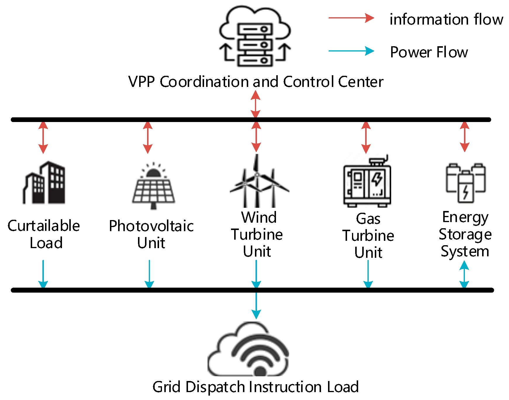
2.1. Structure of the Virtual Power Plant

The VPP constructed in this paper is shown in Figure 1, consisting of photovoltaic power stations, wind turbines, energy storage batteries, gas turbines, and user-side flexible loads. The virtual power plant considered in this paper mainly performs the following two functions:
  • Completing the load plan predetermined with the distribution network:
The primary function of the VPP is to complete the daily load schedule based on the dispatch agreement with the distribution network. The VPP prioritizes the consumption of wind and photovoltaic power, with both having the same priority and being called in parallel. Wind and photovoltaic power are primarily used to meet load demand, ensuring maximum utilization of renewable energy, and avoiding wind and solar curtailment. The remaining power will be optimized based on the overall system situation to determine whether it should be used to charge energy storage or directly sold to the grid.
  • Characterizing the scheduling boundary for intra-day dispatch:
On the basis of fulfilling the pre-scheduled load plan, the virtual power plant uses its remaining regulation potential to characterize its scheduling boundary. When the distribution network has additional intra-day scheduling requirements, it can interact with the virtual power plant based on the provided scheduling boundary to implement demand response.

2.2. VPP Operation Strategy and Scheduling Process

In daily operation, the VPP aims to minimize operating costs by coordinating the distributed energy resources it aggregates in response to the dispatch instructions from the distribution network. In the VPP model constructed in this paper, both wind farms and photovoltaic power plants participate in the scheduling according to their actual output, with forecast data updated every 15 min for the next 4 h. The VPP, based on the latest forecast data, optimizes the scheduling plan and scheduling boundaries for the next 4 h every 15 min, which are then reported to the distribution network. This setting is based on the guidelines provided in reference [32]. Surplus electricity from the VPP will be sent to the grid under the surplus electricity injection strategy. If the VPP’s own output cannot meet the original dispatch instructions from the distribution network, it must report the missing power information to the distribution network’s dispatch center and bear the corresponding unserved load penalty. If the distribution network has additional scheduling demands during real-time operation, dispatch instructions can be issued based on the real-time scheduling boundaries reported by the VPP. The VPP scheduling process is shown in Figure 2.

2.3. Objective Function

The objective is to minimize the total cost over the VPP operation period. The specific expression of the objective function is as follows:
F = t = 1 T F W , t + F PV , t + F ES , t + F MT , t + F CL , t + F Q , t F S , t ,
F W , t = C W P W , t Δ t F PV , t = C PV P PV , t Δ t F ES , t = C ES P ES , t Δ t F MT , t = a MT P MT , t + b MT Δ t F CL , t = C CL P CL , t Δ t F Q , t = C Q P Q , t Δ t F S , t = C sell P sell , t Δ t .

2.4. Constraints

2.4.1. Power Balance Constraint

P WT , t + P PV , t + P ES , t + P MT , t + P Q , t + P CL , t P sell , t = b Δ P G , t + P G , t .

2.4.2. Energy Storage Battery Operation Constraint

P ES , t = P t dis P t char u t char + u t dis 1 0 P t char u t char P char max 0 P t dis u t dis P dis max S t = S t 1 + ( η char P t char P t dis / η dis ) Δ t / E bat S min S t S max S start = S end .

2.4.3. The Reducible Load Constraint

0 P CL , t P C L , t m a x .
In the equation, P C L , t m a x represents the maximum reducible power of the load at time t. The power value is determined by the agreement signed in advance between the virtual power plant and the curtailable load provider. In practice, when the system’s load demand is excessively high, the virtual power plant can reduce a certain proportion of the load according to the agreement, in order to balance the system load and ensure the stable operation of the grid. To compensate for any economic losses that the curtailable load provider may incur during the scheduling process, the virtual power plant will provide corresponding financial compensation based on the pre-agreed compensation standards.

2.4.4. Gas Turbine Constraints

u G T , t P M T m i n P M T , t u G T , t P M T m a x ,
P M T d o w n P M T , t P M T , t 1 P M T u p .

2.4.5. Rotating Reserve Constraint

min ( u GT , t P MT max P M T , t , P M T u p ) + P CL , t max P CL , t + min ( P dis max P ES , t , ( S t S min ) E bat / Δ t η d i s ) r w t P WT , t + r p v P PV , t ,
min ( P MT , t u GT , t P M T min , P M T d o w n ) + P CL , t + min ( P char max + P ES , t , ( S max S t ) E bat / Δ t / η c h a r ) r w t P WT , t + r p v P PV , t .
Equation (8) represents the upward spinning reserve, indicating that the additional output capacity of the VPP is required to compensate for the insufficient wind and solar output. Equation (9) represents the downward spinning reserve, indicating that the VPP’s acceptability of capacity is required to manage the excess wind and solar output.

2.4.6. Surplus Power Feed-In Constraint

0 P sell , t P s e l l m a x .
In the equation, P s e l l m a x represents the maximum power output from the VPP to the grid. The value is determined by the agreement signed in advance between the virtual power plant and the distribution network. When wind and photovoltaic resources are abundant, to avoid the waste of wind and solar energy, the virtual power plant can sell part of the surplus electricity to the grid. The specific amount of electricity to be sold is set by the distribution network based on factors such as its operational demand, supply capacity, and grid security.

3. VPP Time Coupling Treatment and Problem Decomposition

Due to the volatility of renewable energy generation and the temporal coupling inherent in energy storage systems, the optimization problem for VPP becomes complex and resource-intensive, making it difficult to meet the timeliness requirements for day-ahead interactions with the distribution grid. Time decoupling can effectively reduce the scale and complexity of the optimization problem, while distributed optimization further decomposes the problem, improving computational efficiency. Therefore, this paper applies time coupling relaxation and distributed optimization within the VPP to ensure that the internal optimization process meets the timeliness requirements for day-ahead interactions with the distribution grid.

3.1. Overall Design Concept of Distributed Optimization

The optimization objective in this paper is to achieve the optimal total operating cost within the VPP scheduling period, which is a long-term centralized optimization problem. The optimization design process is shown in Figure 3.
The time coupling constraints are mainly composed of the neighborhood time coupling constraints S t = S t 1 + ( η char P t char P t dis / η dis ) Δ t / E bat , which accumulate the energy storage state of charge (SOC), and the wide area time coupling constraint S start = S end , which enhances the scheduling flexibility of energy storage resources. Time coupling indicates that there are interdependencies between different time points in the optimization problem. These constraints increase the complexity and difficulty of solving the problem. This paper uses the Lyapunov optimization theory to achieve time decoupling within the VPP. First, a virtual queue representing the accumulation of the energy storage state SOC is constructed using the Lyapunov function, transforming the energy storage charging and discharging problem into a stability problem of the virtual queue. Then, the corresponding Lyapunov Drift-Plus-Penalty function is introduced to relax and decouple the time coupling constraints, breaking the optimization problem into multiple independent subproblems for each time period. This significantly reduces the complexity of the optimization problem while ensuring local optimality and approaching the global optimal solution. After time decoupling, the optimization solutions between adjacent time periods are shown in Figure 4.
After time decoupling, the problem is ultimately transformed into a distributed optimization problem for multiple time periods using the ADMM distributed framework. Each subproblem is solved using the Hybrid Strategy Particle Swarm Optimization (HSPSO) algorithm to improve computational accuracy and efficiency.

3.2. Lyapunov Optimization-Based Time Decoupling Strategy

Time coupling is caused by the constraints on the SOC of the energy storage system. The neighborhood time coupling constraints are combined and written in the cumulative form from time t = 0 to t = T . By dividing both sides by the period T, we obtain
1 T S t = T = 1 T S start + 1 T t = 1 T u t d i s P t d i s / η d i s η char u t chart P t char / E bat .
Throughout the entire scheduling period, the SOC of the energy storage system at the beginning and end of the period is kept consistent, allowing for continued scheduling in the next period and thereby improving the scheduling flexibility of the energy storage resources, i.e., S t = T = S start . Therefore, the preliminary time coupling relaxation result can be obtained as follows:
1 T t = 1 T u t d i s P t d i s / η d i s η c h a r u t c h a r t P t c h a r / E b a t = 0 .
The above equation represents a preliminary relaxation of the time coupling constraints; however, the problem remains complex and difficult to solve. Therefore, a virtual queue is established to reflect the accumulated SOC of the energy storage system:
Q t = Q t 1 + u t d i s P t d i s / η d i s η c h a r u t c h a r t P t c h a r / E b a t
At this point, both the wide area coupling constraints and neighborhood coupling constraints in the VPP internal optimization are transformed into the stability problem of the virtual queue. In this paper, the Lyapunov function is introduced to represent the stability of the virtual queue:
H t = Q t 2 2 .
To better measure the stability characteristics and evolution trends of the virtual queue, the Lyapunov drift function is further calculated. Δ H t is used to represent the difference in congestion levels of the virtual queue between adjacent time steps:
Δ H t = H t + 1 H t .
According to the properties of the drift function, for the virtual queue to tend toward stability, Δ H t should be minimized as much as possible.

3.3. Optimization Problem Transformation Based on Drift Plus Penalty

To simultaneously balance the stability of the virtual queue and the objective function of the VPP internal optimization, the Drift Plus Penalty (DPP) function, as introduced in [33], is used to transform the long-term centralized optimization problem into a single-period centralized optimization problem. This transforms the original objective function into the minimization of the value F t r for each time period:
min F t r = ζ Δ H t + F t .
The above equation can be seen as a trade-off between the stability of the virtual queue and the operating cost of the VPP. Substituting Equations (13)–(15) into Equation (16), we obtain
F t r = ζ 2 Δ S t 2 + ζ Q t Δ S t + F t ,
F t r ζ 2 Δ S t m a x 2 + ζ Q t Δ S t + F t .
From Equation (18), it can be observed that F t r has an upper bound, and ζ Δ S t m a x 2 in the upper bound is a constant. Therefore, the above problem can be regarded as minimizing ζ Q t Δ S t + F t , where ζ Q t Δ S t represents the penalty for violating the energy storage state-of-charge constraints. Consequently, Equation (16) can be reformulated as follows:
min F t r = ζ Q t Δ S t + F t .
Δ S t represents the variation in the SOC of the energy storage system. At this point, the temporal decoupling of constraints caused by the SOC limitations of energy storage systems has been achieved, relaxing both the global and local temporal coupling constraints. This transforms the long-term centralized optimization problem into a single-period centralized optimization problem. It is important to note that after temporal decoupling, the level of information exchange between different time periods diminishes, which may result in the partial loss of global information and consequently some degree of optimality degradation. However, in the context of real-time scheduling for virtual power plants, computational efficiency and real-time performance are typically regarded as more critical metrics than achieving global optimality. Furthermore, this loss of optimality is generally within an acceptable range and does not significantly impact the overall system performance.

3.4. The Distributed Optimization Solution Method Based on ADMM-HSPSO

3.4.1. Optimization Problem Decomposition Based on ADMM

For the single-period centralized optimization problem, an augmented Lagrangian function is first constructed. The constraints of the optimization problem are incorporated into the objective function via their corresponding dual multipliers, transforming the original problem into an unconstrained optimization problem:
L t P i , t , z , λ t = F t r + C ( P i , t , z ) T λ t + β 2 C ( P i , t , z ) 2 .
Using the ADMM algorithm framework, the problem is decomposed into two subproblems. The first subproblem optimizes the continuous variable P i , t , while treating the relaxation variable z and the dual variable λ as constants. The first subproblem can be expressed as follows:
P i , t k + 1 = arg min P i , t k L t P i , t k , z t k , λ t k .
The second subproblem involves updating the relaxation variable, which is used to coordinate interactions among multiple subproblems and ensure consistency between local decisions and global requirements. At this stage, the original variable P i , t and the dual variable λ are treated as constants, while the auxiliary variable z is optimized. The second subproblem can be expressed as follows:
z t k + 1 = arg min z t k L t P i , t k + 1 , z t k , λ t k .
The update of the dual variable is used to dynamically adjust the degree of constraint violation and guide the optimization process toward convergence through a feedback mechanism. The update method is expressed as follows:
λ t k + 1 = λ t k + C ( P i , t k + 1 , z t k + 1 ) .
At this point, the ADMM algorithm framework has further reduced the scale of the optimization problem, thus improving computational efficiency and laying the foundation for the next step of centralized algorithm optimization of the subproblems.

3.4.2. Subproblem Solving Based on Hybrid Strategy Improved PSO Algorithm

The particle swarm optimization (PSO) algorithm, as a classic intelligent optimization method, has been extensively studied. Therefore, its mathematical model will not be elaborated upon in this paper. To address the common challenges of PSO, including sensitivity to initial values, slow convergence speed, and susceptibility to local optima, improvement strategies are proposed as follows:
  • Step 1: Sobol Sequence-Based Population Initialization
This study utilizes Sobol sequence-based population initialization as a replacement for traditional random initialization. This approach ensures a more uniform distribution of the initial population, covering a broader solution space, thereby reducing the impact of initial values on the computation results [34]. The population distribution of Sobol sequence initialization and random initialization is illustrated in Figure 5.
  • Step 2: Adaptive Inertia Weight
The standard PSO algorithm employs a fixed inertia weight, which may result in low efficiency. To fully leverage the advantages of PSO, this study adopts an adaptive weight strategy, allowing the inertia weight to be dynamically adjusted during the iteration process. [35]. This approach optimizes the balance between global exploration and local exploitation, thereby accelerating the convergence process. The weight update expression is as follows:
ω i d = ω min + ω max ω min f x i d f min d f a v e r a g e d f min d , f x i d f a v e r a g e d ω max , f x i d > f a v e r a g e d .
During the iteration process, the fitness of particles is continuously compared with the average fitness, allowing for flexible adjustment of the weight values to accelerate convergence.
  • Step 3: Adaptive Cauchy Mutation Strategy
Although the aforementioned improvement measures reduce the likelihood of the algorithm falling into local optima to some extent, a certain probability still exists. To further mitigate this issue, this study introduces an adaptive Cauchy mutation strategy, which perturbs the current optimal solution to enhance the algorithm’s global search capability [36]. The details are as follows:
Δ f x i d = 1 f x i d f x i d 6 0.1 × f x i d 6 0 otherwise ,
P ( x d ) = i = 1 N Δ f x i d / N ,
M x d = 1 P x d S 0 P x d < S .
In the equations P ( x d ) denotes the proportion of all particles trapped in local optima at the t -th iteration; S is the threshold for determining whether the algorithm has fallen into a local optimum at the d -th iteration, which is set to 0.6 based on multiple tests; and M x d is the flag value indicating whether the algorithm has fallen into a local optimum at the d -th iteration.
After determining that the algorithm has fallen into a local optimum, a Cauchy mutation is applied to the current optimal solution. Its mathematical expression is as follows:
G b e s t n e w d = G b e s t d × 1 + c a u c h y ( 0 , 1 ) .
In the formula G b e s t n e w d represents the new value of the optimal solution after undergoing Cauchy mutation in the d -th iteration; c a u c h y ( 0 , 1 ) denotes the standard Cauchy distribution. After obtaining G b e s t n e w d , the algorithm compares the fitness values of G b e s t n e w d and G b e s t d . If G b e s t n e w d outperforms G b e s t d , the current optimal solution is replaced by G b e s t n e w d ; otherwise, no replacement occurs.

4. Interaction Between Dispatch Boundary and Distribution Network

4.1. Subsection Virtual Power Plant Dispatch Command Analysis

The characterization of the dispatch boundary in this study is based on dispatch instructions, which are also divided by time intervals and solved step by step. Consequently, with time decoupling, the real-time characterization of the dispatch boundary is supported by fast computation. The VPP dispatch boundary is established on the basis of meeting the day-ahead dispatch plan, representing the remaining adjustment potential of the VPP. This remaining adjustment capacity is then utilized to respond to additional intraday dispatch requests from the distribution network, further promoting interaction with the distribution network and enhancing both efficiency and utilization. The interaction process is illustrated in Figure 6.
During the intraday period, the distribution network issues a new dispatch instruction t s , t c , P G , which includes the dispatch start time t s , the duration of the dispatch instruction t c , and the dispatch power Δ P G . The constraints for the start time t s and duration t c are as follows:
1 t c 16 t s min t s t s min + 15 t s min + 1 t c + t s t s min + 16 .
In this context, t s min denotes the minimum start time for a dispatch instruction, while t c , t s , and t s min are all integers. For example, t s , t c , Δ P G = 5 , 4 , 6 represents a dispatch instruction starting at 1:15 (with 15 min intervals per time slot, where a day consists of 96 slots and the 5th slot corresponds to 1:15–1:30), lasting 4 slots, equivalent to 1 h, during which the virtual power plant increases its output by 6 MW. The optimization time window in this study spans 4 h, encompassing 16 time slots. Thus, the dispatch instruction can begin at any of 16 time points. If the duration of the dispatch instruction is 1 slot ( t c = 1 ), there are 16 possible schemes; if t c = 2 , there are 15 schemes, and so on. This results in a total of 136 combinations. Each combination must be analyzed to determine the corresponding dispatch boundary. The dispatch boundary characterization in this study focuses on continuous dispatch instructions. However, the complete dispatch boundary of the virtual power plant also includes non-continuous instructions and their combinations. Consequently, the total number of possible dispatch boundary combinations significantly exceeds 136.
Due to the time continuity in executing dispatch instructions, both multiple instructions within the same time period and non-continuous dispatch instructions can be implemented based on the foundation of these 136 continuous dispatch boundaries. When the distribution network requires dispatch across non-continuous time periods, it can decompose the combined instructions into multiple continuous dispatch instructions:
D t t , Δ P G ,
t t represents the specific number of time periods, where t t ( t 1 , t 2 , t k ) and t 1 < t 2 < t k . The decomposition of instructions into a set of multiple continuous instructions is as follows:
D t s 1 , t c 1 , Δ P G , t s 2 , t c 2 , Δ P G , , t s 3 , t c 3 , Δ P G .
For example, D ( 1 , 2 , 5 , 8 , 9 ) , ( 2 ) can be decomposed into three continuous instructions executed sequentially: (1,2,2), (5,1,2), and (8,2,2).

4.2. Wind–Solar Fluctuation Factor and Dispatch Boundary Characterization

To address the challenges posed by the intermittency and volatility of renewable energy output in characterizing the scheduling boundaries of a VPP, this paper introduces the Wind–Solar Fluctuation Factor as a metric to quantify the degree of fluctuation. The Wind–Solar Fluctuation Factor is determined by gradually amplifying the wind and solar fluctuation amplitudes to test the VPP’s maximum regulation potential under varying fluctuation conditions, thereby quantifying its remaining regulation capability (i.e., the dynamic changes in the scheduling boundaries). This factor reflects the VPP’s regulation limits under extreme fluctuation conditions, revealing the scheduling margin of the system in different fluctuation scenarios. The inequality constraints in Equations (8) and (9) are, respectively, transformed into the following:
min ( u GT , t P M T max P MT , t , P M T u p ) + P CL , t max P CL , t + min ( P dis max P ES , t , ( S t S min ) E bat / Δ t η d i s ) ψ 1 i ,
min ( P MT , t u GT , t P M T min , P M T d o w n ) + P CL , t + min ( P char max + P ES , t , ( S max S t ) E bat / Δ t / η c h a r ) ψ 2 i .
In the equation ψ 1 i and ψ 2 i represent the Wind–Solar Fluctuation Factors for the i -th scheduling scenario, respectively. By assigning evenly spaced values to ψ 1 i and ψ 2 i , the calculation of the upper scheduling boundary requires only meeting the baseline wind–solar fluctuations, i.e., satisfying Equations (9) and (32). If a solution exists, the value of ψ 1 i is incrementally increased until no solution is found. The calculation of the lower boundary follows the same principle. The maximum Wind–Solar Fluctuation Factors that satisfy the constraints are determined, and the capacity required to handle standard wind–solar fluctuations (consistent with ultra-short-term forecasting standards) is subtracted. The remaining portion is equivalent to the residual adjustable capacity of the VPP for that time period, which defines the upper and lower scheduling boundaries as follows:
P up i = ψ 1 i r WT P WT , t + r PV P PV , t ,
P down i = ψ 2 i r WT P WT , t + r PV P PV , t .
In the equation P up i and P down i represent the upper and lower boundaries for the i -th scheduling scenario, respectively. The flowchart for the scheduling boundary characterization process is shown in Figure 7.

5. Case Analysis

5.1. Case Parameter Settings

Taking the data of a VPP in a specific region as an example, the load curve of the day-ahead typical day scheduling instructions and the wind–solar power output forecast are shown in Figure 8. Key computational parameters required for the optimization are presented in Table 2. The operating parameters of the units within the VPP refer to Reference [37], as listed in Table 3. The wind–solar power output prediction error coefficients are determined based on the Reference [32]. The maximum reducible load output is set to 10% of the day-ahead scheduling instruction load curve. Figure 9 illustrates the scheduling plan of each unit within the VPP when no new scheduling instructions are issued by the distribution network, with a scheduling cost of CNY 36,567. In intra-day optimization scheduling, the wind and photovoltaic outputs fluctuate within ranges of 13% and 10%, respectively, to simulate the uncertainty of wind and solar output. All case studies and tests were conducted using MATLAB 2018b on a system equipped with an Intel(R) Core(TM) i5-8300H processor and 8 GB of RAM, sourced from ASUS, Chengdu, China.

5.2. Effectiveness and Feasibility Verification of Time Decoupling

5.2.1. Validation of Time Decoupling Effectiveness

To verify the effectiveness of time decoupling, the day-ahead scheduling plan data of a VPP is used. The optimization period is selected as time intervals 41 to 48, corresponding to 10:00–12:00, to serve as the validation period for VPP time decoupling. Optimization is conducted without new scheduling instructions from the distribution network, without delineating the VPP scheduling boundary, and without calculating scheduling costs. This demonstrates the necessity of time decoupling and the computational efficiency achieved after decoupling. The scenarios in this study are as follows.
Scenario 1: The optimization problem is solved without applying time decoupling.
Scenario 2: The optimization problem is solved with time decoupling applied.
The optimization is performed every 15 min, covering a total of 8 optimization intervals. The number of objective functions and constraints before and after time decoupling is shown in Table 4.
Before decoupling, the constraints and variables for all eight intervals must be considered simultaneously. Each interval includes 15 constraints (after simplification and consolidation) and 4 variables, resulting in a total of 120 constraints and 32 variables. After decoupling, it is only necessary to compute the minimum for each time step sequentially and sum up the results. The optimization results obtained through repeated calculations are shown in Figure 10.
As shown in Figure 10, the computation time before decoupling was 36 s, with an operational cost of CNY 6405. After decoupling, the computation time was reduced to 5 s, and the operational cost increased slightly to CNY 6429—an increase of only CNY 24, accounting for less than 0.4%. Decoupling reduced the computation time by 86.11%, significantly decreasing computation time. In intraday real-time optimization, scheduling plans for the next 4 h must be optimized every 15 min. This process involves up to 240 constraints and 64 variables, leading to a sharp increase in computational complexity. Additionally, the virtual power plant’s scheduling boundaries and operational costs must also be calculated, making it difficult to meet the timeliness requirements of intraday dispatch.

5.2.2. Feasibility Validation of Time Decoupling

To verify the feasibility of time decoupling in VPP, this paper uses the day-ahead scheduling plan of a VPP as a case study to calculate the operational cost for one day. Additionally, a quantitative analysis is performed to assess the optimality loss caused by time decoupling. For this purpose, scenarios three, four, and five are set up for comparative analysis.
Scenario 3: Time decoupling using hourly optimization.
Scenario 4: Time decoupling using Lyapunov optimization.
Scenario 5: Direct optimization without time decoupling.
The number of iterations is set to 1000, with all scenarios being computed three times, and the average of the results is taken. The operational cost of the virtual power plant is shown in Figure 11.
According to the virtual power plant operating cost analysis in Figure 11, when time decoupling is performed using hourly optimization, the total operating cost of the virtual power plant for the entire period is CNY 37,981, with an error of 6.8% compared to the case without time decoupling. When Lyapunov optimization is applied for time decoupling, the operating cost is CNY 36,378, with an error of only 2.3%. Compared to hourly optimization, Lyapunov optimization reduces the optimality loss by 66.27%. This is because Lyapunov optimization utilizes accumulated information from the past SOC of energy storage devices to guide the optimization at the current time step, compensating for the lack of global information to some extent and reducing the optimality loss caused by time decoupling. The cost for full-period optimization is CNY 35,562, which is the lowest operating cost among the three methods. The reason is that full-period optimization does not require segmented solving, thus avoiding the global information loss caused by decoupling.
In terms of computation time, the calculation times for Lyapunov optimization and hourly optimization are 42 s and 45 s, respectively, with only a slight difference. In contrast, the computation time for full-period optimization is as high as 2385 s. This is because both Lyapunov optimization and hourly optimization decompose the optimization problem into multiple periods to be solved individually, reducing the complexity of the optimization problem. In contrast, full-period optimization requires considering all variables and constraints throughout the entire period simultaneously, and there are interdependencies between variables and constraints at different time nodes, resulting in a much larger-scale optimization problem. This requires a longer computation time to converge with a stable result.
In summary, although time decoupling may result in some optimality loss, the error of the time decoupling strategy based on Lyapunov optimization is less than 3%, which is acceptable in practical applications. In the intraday optimization of a virtual power plant, greater emphasis is placed on timeliness and the feasibility of the solution. Time decoupling significantly reduces the optimization complexity and improves solving efficiency. Therefore, the time decoupling strategy is both feasible and of practical value in virtual power plants.

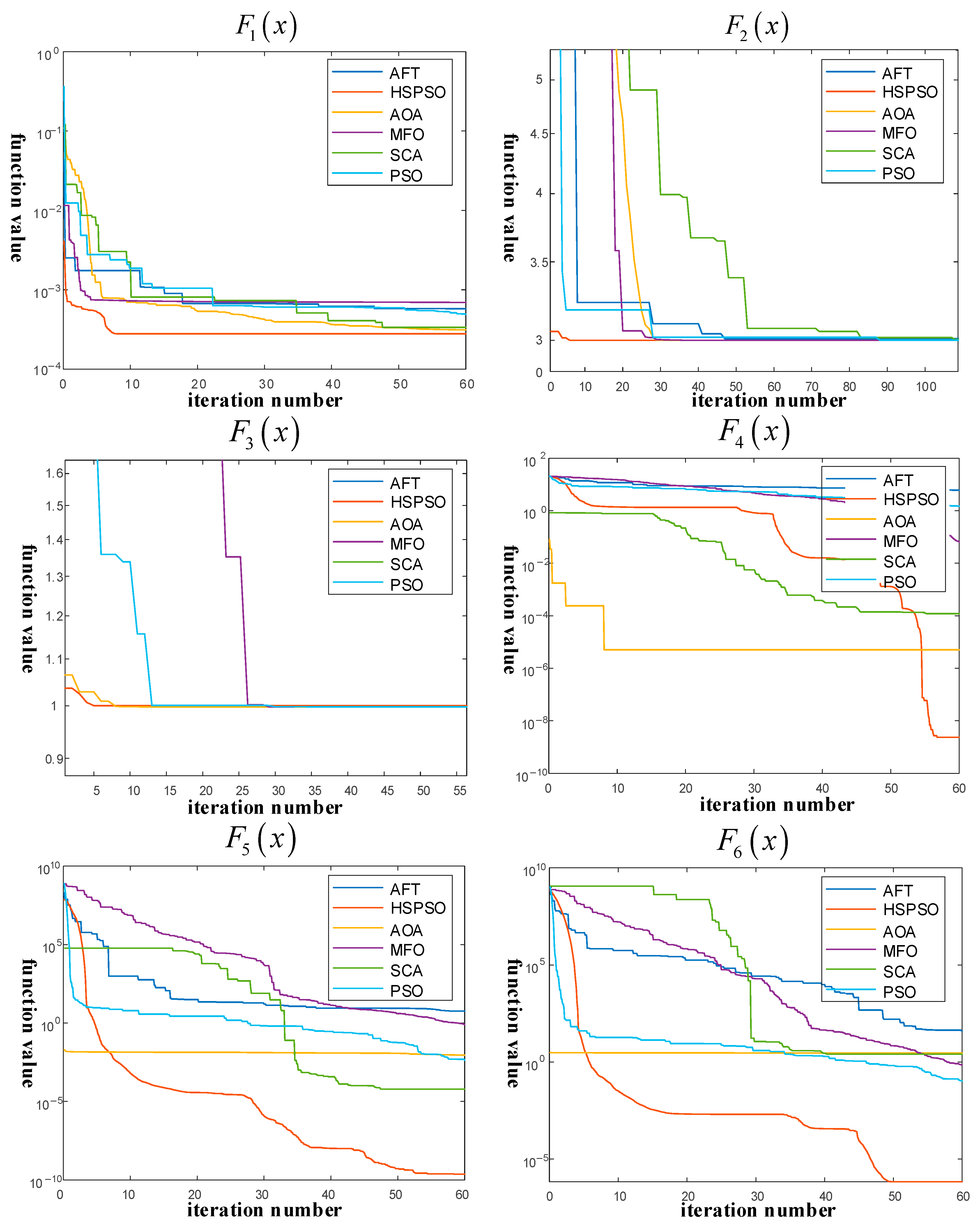
5.3. HSPSO Algorithm Performance Analysis and Validation

To validate the effectiveness of the HSPSO algorithm, it is compared with commonly used intelligent algorithms such as the Arithmetic Optimization Algorithm (AOA), Moth Flame Optimization Algorithm (MFO), Sine Cosine Algorithm (SCA), Ali Baba and Forty Thieves Algorithm (AFT), and PSO. Six classical benchmark functions, including both unimodal and multimodal functions, are used for testing. Detailed information about the test functions and algorithm parameter settings can be found in Appendix A. The maximum number of iterations for all algorithms is set to 600, with a population size of 30. Each algorithm is independently run 30 times, and the average convergence curve is shown in Figure 12.
As shown in Figure 12, the HSPSO algorithm exhibits minimal differences compared to other algorithms in unimodal functions, as the simple structure of unimodal problems allows for rapid convergence to the global optimal solution. However, in the optimization of multimodal functions, the HSPSO algorithm demonstrates a significant advantage, achieving higher computational accuracy than other algorithms. The hybrid strategy improves the algorithm by effectively enhancing population diversity and avoiding premature convergence. In contrast, other algorithms show lower computational accuracy in multimodal problems due to insufficient exploration capability.

5.4. Analysis of Dispatch Boundary Characterization

5.4.1. Results Analysis of Dispatch Boundary Characterization

Taking the 2nd and 17th time periods (i.e., 00:15–04:15, a 4 h duration) as an example, the scheduling boundary is depicted. Figure 13 illustrates the scheduling boundary of the virtual power plant during this period.
To ensure the safe and reliable operation of the virtual power plant, all scheduling boundaries depicted in this paper are rounded down to provide a certain margin. In the 4 h scheduling boundary depicted, there are a total of 136 scheduling scenarios. Taking the instruction start time period of 16 and instruction duration of 2 as an example (i.e., 03:45–04:15), the virtual power plant can increase power output by up to 3 MW or decrease it by up to 1 MW based on the original scheduling instructions.
The virtual power plant constructed in this paper not only provides scheduling boundaries to the distribution network but also offers the associated scheduling costs of these boundaries. This enables the distribution network to comprehensively evaluate whether to interact with the virtual power plant. The scheduling costs of the virtual power plant are shown in Figure 14.
Taking the instruction start time period of 5 and a duration of 2 as an example (i.e., 01:00–01:30), the virtual power plant can increase power output by up to 3 MW or reduce it by up to 1 MW. Reducing power by 1 MW decreases the cost by CNY 103, while increasing power by 1 MW, 2 MW, and 3 MW incurs costs of CNY 137, CNY 352, and CNY 526, respectively. Through time decoupling and optimization algorithm improvements, the boundary depiction and scheduling cost calculation can be completed within a short time, laying the foundation for the efficient operation and real-time interaction of the virtual power plant. The total time for scheduling boundary depiction is 115 s, and the total time for scheduling cost calculation is 6.7 s, effectively meeting the timeliness requirements for interactions between the virtual power plant and the distribution network.

5.4.2. Comparison of Virtual Power Plant Optimization and Interaction with the Distribution Network

With the rapid development of data-driven technologies, methods based on machine learning and reinforcement learning have been widely applied to virtual power plant optimization scheduling and interaction with the distribution network. To compare and analyze the performance of the method proposed in this paper with data-driven methods in optimization scheduling and interaction with the distribution network, we selected two methods for comparison:
Method A: The virtual power plant scheduling method based on Lyapunov optimization proposed in this paper.
Method B: The data-driven virtual power plant optimization scheduling method, as detailed in Reference [21], which will not be further elaborated in this paper.
Using a 4 h time scale as an example, we implement the characterization of the virtual power plant scheduling boundary and cost calculation. The results are shown in Table 5.
As shown in Table 5, the overall model update and training time is 98 s, with the model solving time and total time amounting to 113 s. The total time is approximately 7% shorter than the method proposed in this paper, indicating a minimal difference between the two. The main time-consuming aspect of the data-driven method lies in model updates and training, which account for 86.7% of the total time. Furthermore, this method requires continuous updates of training data to maintain model accuracy. Additionally, data-driven methods often lack transparency, making the decision-making process unclear to operators. In contrast, the scheduling method based on Lyapunov optimization proposed in this paper provides a clear decision-making process (with each scheduling boundary derived from actual calculations), avoiding the issues of over-reliance on data and lack of transparency that may arise with data-driven methods. Moreover, as indicated in Reference [21], the method in this paper has advantages in terms of scheduling boundary reliability and ease of interaction with the distribution network.

5.4.3. Comparison of Dispatch Boundary Characterization Methods

To further verify the reliability of the virtual power plant scheduling boundary characterization method proposed in this paper, and the feasibility of the distribution network issuing scheduling instructions based on this scheduling boundary, we compared it with the method in Reference [27]. Reference [27] generated a large number of wind and solar output scenarios based on the probability density function of renewable energy output, and it calculated the proportion of scenarios that meet the demand to obtain the execution probability of the scheduling boundary. We compared and analyzed the method in Reference [27] with the scheduling boundary characterization method proposed in this paper.
To obtain the probability density function of the renewable energy output, this paper uses the Gaussian kernel density estimation method. Based on a large amount of historical data, we derive the probability density functions of the intra-day ultra-short-term forecast errors for wind power and photovoltaic generation, as shown in Figure 15. Figure 16 displays 1000 wind and solar output scenarios randomly generated using the Monte Carlo method based on this forecast error probability density function, to simulate the uncertainty of wind and solar output.
Similarly, taking the 2nd and 17th time periods (i.e., 00:15–04:15, a 4 h duration) as an example, the scheduling boundaries are depicted. Using an instruction start time period of 14 and a duration of 1 period as an example, the scheduling boundary results are shown in Table 6.
As shown in Table 6, the scheduling boundaries depicted using the scenario generation method are broader. However, these boundaries are based on certain probabilities, and the method cannot guarantee that the virtual power plant can respond to all dispatch instructions issued by the distribution network within these boundaries. The scheduling boundaries proposed in this paper are relatively conservative. If the intraday wind and photovoltaic forecast data meet the national standard requirements referenced in this study, complete response to dispatch instructions can be achieved within the depicted boundaries, thus meeting the requirements for dispatch reliability.
In addition, the scenario generation method requires the Monte Carlo approach to generate numerous scenarios, followed by optimization calculations for each scenario. This results in a high computational burden, making it challenging to meet the timeliness requirements for intraday interactions. Therefore, the method proposed in this paper better satisfies the distribution network’s requirements in terms of both efficiency and reliability for scheduling boundary depiction.

6. Conclusions

This paper aims to improve the operational efficiency of virtual power plants, optimize operating costs, and quickly and reliably characterize the VPP scheduling boundary, thereby promoting efficient interaction between the VPP and the distribution network. To achieve this goal, this paper proposes a time-decoupling strategy based on Lyapunov optimization, and solves it using the ADMM distributed optimization framework combined with a hybrid strategy-improved Particle Swarm Optimization algorithm. The main conclusions are as follows:
(1)
Through the Lyapunov optimization theory, this paper successfully implements time decoupling within the virtual power plant, transforming the long-term optimization problem into multiple single-period optimization problems, which significantly reduces the complexity of the optimization problem. Taking a 2 h intra-day optimization scheduling for the VPP as an example, the solving time after decoupling is reduced by 86.11%, and the overall daily operational cost error is only 2.4%, which validates the feasibility and effectiveness of this strategy.
(2)
The hybrid strategy improved Particle Swarm Optimization algorithm proposed in this paper shows significant advantages in both computational accuracy and solving speed. Test results demonstrate that the algorithm converges in fewer than 15 iterations for unimodal tests, and achieves an accuracy of 10−5 or better in multimodal tests, proving the efficiency and superiority of this algorithm.
(3)
Compared to the scenario generation method based on probability density functions, the scheduling boundary characterization method proposed in this paper offers higher reliability and computational efficiency. For example, for the 4 h period from 00:15 to 04:15, the scheduling boundary is characterized in 115 s with an execution probability of 100%. In contrast, the scenario generation method cannot guarantee a 100% execution probability for the scheduling boundary, and requires analysis and calculation for each scenario, making it difficult to meet the timeliness requirements for intra-day interactions.
Although this paper primarily focuses on the internal optimization of the VPP and its interaction with the distribution network, future research could extend the application of VPP in the electricity market, including spot and futures markets, as well as ancillary services such as peak shaving and frequency regulation. Additionally, future studies could consider incorporating more controllable resources and uncertainty factors to enhance the adaptability of the methods and the robustness of the system. In particular, given the increasing use of grid-forming inverters in recent years, future research will explore how to integrate the frequency and voltage constraints of grid-forming inverters into the optimization model and examine whether this approach can produce effective results while allowing for an optimal solution.

Author Contributions

Conceptualization, Y.F. and J.Y.; methodology, J.Y.; validation, J.Y. and Y.F.; formal analysis, J.Y.; investigation, J.H.; resources, J.H.; data curation, J.Y.; writing—original draft preparation, J.Y.; writing—review and editing, J.Y.; visualization, J.Y.; supervision, J.H.; project administration, Y.F.; funding acquisition, Y.F. All authors have read and agreed to the published version of the manuscript.

Funding

This work has been supported by the Natural Science Foundation of Xinjiang Uygur Autonomous Region under 2022D01C365, and the Tianshan Talent Training Program under 2022TSYCLJ0019.

Data Availability Statement

The original contributions presented in the study are included in the article, further inquiries can be directed to the corresponding authors.

Conflicts of Interest

The authors declare no conflicts of interest.

Appendix A

Table A1. Mathematical expression.
Mathematical Expression
F 1 x = i = 1 11 a i x 1 b i 2 + x 2 b i b i 2 + x 3 b i + x 4 2
F 2 x = 1 + x 1 + x 2 + 1 2 19 14 x 1 + 3 x 1 2 14 x 2 + 6 x 1 x 2 + 3 x 2 2 × 30 + 2 x 1 3 x 2 2 18 32 x 1 + 12 x 1 2 + 48 x 2 36 x 1 x 2 + 27 x 2 2
F 3 x = 1 500 + j = 1 25 1 j + i = 1 2 x i c i j 6 1
F 4 x = 20 exp 0.2 1 n i = 1 n x i 2 exp 1 n i = 1 n cos 2 π x i + 20 + e
F 5 x = π n 10 sin π y 1 + i = 1 n 1 y i 1 2 1 + 10 sin 2 π y i + 1 + y n 1 2 + i = 1 n U f u n x i , 10 , 100 , 4 y i = 1 + x i + 1 4
F 6 x = 0.1 sin 2 ( 3 π x 1 ) + i = 1 n 1 x i 1 2 1 + sin 2 3 π x i + 1 + x n 1 2 1 + sin 2 2 π x n + i = 1 n U f u n x i , 5 , 100 , 4
Individual parameters in Table A3 are described as follows:
a = 0.1957 , 0.1947 , 0.1735 , 0.16 , 0.0844 , 0.0627 , 0.0456 , 0.0342 , 0.0323 , 0.0235 , 0.0246 ,
b = 1 0.25 , 0.5 , 1 , 2 , 4 , 6 , 8 , 10 , 12 , 14 , 16 ,
c = 32 , 16 , 0 , 16 , 32 , 2 , 16 , 0 , 16 , 32 , 32 , 16 , 0 , 16 , 32 , 32 , 16 , 0 , 16 , 32 , 32 , 16 , 0 , 16 , 32 ; 32 , 32 , 32 , 32 , 32 , 16 , 16 , 16 , 16 , 16 , 0 , 0 , 0 , 0 , 0 , 16 , 16 , 16 , 16 , 16 , 32 , 32 , 32 , 32 , 32 ,
U f u n x i , a , k , m = k x i a m x i > a 0 a < x i < a k x i a m x i < a .
Table A2. Parameter settings for each algorithm.
AlgorithmParameter
AFTInitial value of perceived potential: 0.15
Initial value of tracking distance: 1.5
MFOControl search intensity: −1
Step size influence factor: 1
AOAConvergence parameters:7, adjustment amplitude: 0.2
maximum/small target probability: 0.8/0.3
SCAControl convergence rate: 2
PSO ω max = 0.9 , ω min = 0.4 , c 1 = 2 , c 2 = 2
Table A3. Test function parameters.
Function IndexTypeDimensionalityValue RangeOptimal Value
F 1 x unimodal function4 [ 5 , 5 ] 0.0003
F 2 x unimodal function2 [ 2 , 2 ] 3
F 3 x unimodal function2 [ 65 , 65 ] 1
F 4 x multimodal function30 [ 32 , 32 ] 0
F 5 x multimodal function30 [ 50 , 50 ] 0
F 6 x multimodal function30 [ 50 , 50 ] 0

References

  1. Kaiss, M.; Wan, Y.; Gebbran, D. Review on Virtual Power Plants/Virtual Aggregators: Concepts, applications, prospects and operation strategies. Renew. Sustain. Energy Rev. 2025, 211, 115242. [Google Scholar] [CrossRef]
  2. Jin, W.; Wang, P.; Yuan, J. Key Role and Optimization Dispatch Research of Technical Virtual Power Plants in the New Energy Era. Energies 2024, 17, 5796. [Google Scholar] [CrossRef]
  3. Gao, H.; Jin, T.; Feng, C.; Li, C.; Chen, Q.; Kang, C. Review of virtual power plant operations: Resource coordination and multidimensional interaction. Appl. Energy 2024, 357, 122284. [Google Scholar] [CrossRef]
  4. Zhou, S.; Zhang, Y.; Dai, Y. Combined optimization scheduling of virtual power plant including tram. Autom. Instrum. 2024, 11, 125–129. [Google Scholar]
  5. Xu, Y.; Xu, Y.; Yang, J. Low-carbon economic dispatch of electricity-to-gas virtual power plant based on ladder carbon trading. J. Power Syst. Autom. 2023, 35, 118–128. [Google Scholar]
  6. Song, J.; Yang, Y.; Xu, Q.; Liu, Z.; Zhang, X. Robust bidding game approach for multiple virtual power plants participating in day-ahead electricity market. Electr. Power Autom. Equip. 2019, 43, 77–85. [Google Scholar]
  7. Su, H.; Wang, X.; Ding, Z. Bi-Level Optimization Model for DERs Dispatch Based on an Improved Harmony Searching Algorithm in a Smart Grid. Electronics 2023, 12, 4515. [Google Scholar] [CrossRef]
  8. Liu, Z.; Zhao, J.; Tao, W.; Ai, Q. Optimization Scheduling of Combined Heat–Power–Hydrogen Supply Virtual Power Plant Based on Stepped Carbon Trading Mechanism. Electronics 2024, 13, 4798. [Google Scholar] [CrossRef]
  9. Wang, Y.; Lin, H.; Lam, J.; Kwok, K.W. Differentially private consensus and distributed optimization in multi-agent systems: A review. Neurocomputing 2024, 597, 127986. [Google Scholar] [CrossRef]
  10. Zhu, J.; Dong, H.; Li, S.; Zhong, Z.; Chen, Z.; Wu, W. Review of Optimal Dispatching for the Aggregation of Micro-energy Grids Based on Distributed New Energy. Proc. CSEE 2024, 44, 7952–7970. [Google Scholar]
  11. Yang, J.; Hou, J.; Liu, Y.; Zhang, H. Distributed Cooperative Control Method and Application in Power System. Acta Electrotech. 2021, 36, 4035–4049. [Google Scholar]
  12. Chen, H.; Wang, Z.; Zhang, R.; Jiang, T.; Li, X.; Li, G. Decentralized optimal dispatching modeling for wind power integrated power system with virtual power plant. Proc. CSEE 2019, 39, 2615–2625. [Google Scholar]
  13. Kou, L.; Wu, M.; Li, Y.; Qu, X.; Xie, H. Optimization and control method of distributed active and reactive power in active distribution network. Proc. CSEE 2020, 40, 1856–1865. [Google Scholar]
  14. Siqin, Z.; Qiao, T.; Diao, R.; Wang, X.; Xu, G. Research on the Collaborative Operation of Diversified Energy Storage and Park Clusters: A Method Combining Data Generation and a Distributionally Robust Chance-Constrained Operational Model. Electronics 2024, 13, 4997. [Google Scholar] [CrossRef]
  15. Lu, W.; Liu, M.; Lin, S.; Li, L. Incremental-oriented ADMM for distributed optimal power flow with discrete variables in distribution networks. IEEE Trans. Smart Grid 2019, 10, 6320–6331. [Google Scholar] [CrossRef]
  16. Zang, Y.; Xia, S.; Li, J. A robust game optimization scheduling method for shared energy storage micro electric network group distribution. Power Syst. Prot. Control 2023, 51, 90–101. [Google Scholar]
  17. Guo, Z.; Li, G.; Zhou, M. Fast and dynamic robust optimization of integrated electricity-gas system operation with carbon trading. Power Syst. Technol. 2020, 44, 1220–1228. [Google Scholar]
  18. Fan, S.; He, G.; Zheng, X. Research on online distributed optimization-based self-approaching optimization operation method of Virtual Power Plant. Proc. CSEE 2023, 43, 4935–4950. [Google Scholar]
  19. Xu, Z.; He, J.; Liu, Z.; Chen, W.; Wang, X.; Zhang, P. Solution method of virtual power plant dynamic feasible region based on decoupling of coupling constraints. Proc. CSEE 2024, 44, 3440–3452. [Google Scholar]
  20. Sheng, W.; Li, P.; Duan, Q.; Li, Z.; Zhu, C. Research on Energy Management Strategy of Energy Hub with Energy Router Based on Lyapunov Optimization Method. Proc. CSEE 2019, 39, 6212–6225. [Google Scholar]
  21. Hao, R.; Fan, Y.; Hou, J.; Bai, X.; Liu, Y. Construction method of virtual power plant interaction model based on WKNN and KELM-GPR. Acta Energiae Solaris Sin. 2024, 45, 637–649. [Google Scholar]
  22. Chen, X.; Pei, W.; Deng, W.; Zhao, J.; Wang, X.; Pu, T. Data-driven Virtual Power Plant Dispatching Characteristic Packing Method. Proc. CSEE 2021, 41, 4816–4828. [Google Scholar]
  23. Lu, X.; Qiu, J.; Zhang, C.; Lei, G.; Zhu, J. Assembly and Competition for Virtual Power Plants with Multiple ESPs Through a “Recruitment–Participation” Approach. IEEE Trans. Power Syst. 2024, 39, 4382–4396. [Google Scholar] [CrossRef]
  24. Lu, X.; Qiu, J.; Zhang, C.; Lei, G.; Zhu, J. Seizing unconventional arbitrage opportunities in virtual power plants: A profitable and flexible recruitment approach. Appl. Energy 2024, 358, 122628. [Google Scholar] [CrossRef]
  25. Riaz, C.; Mancarella, P. On feasibility and flexibility operating regions of virtual power plants and TSO/DSO interfaces. In Proceedings of the 2019 IEEE Milan Power Tech, Milan, Italy, 23–27 June 2019; pp. 1–6. [Google Scholar]
  26. Liu, Y.; Wu, L.; Chen, Y.; Li, J. Integrating high DER-penetrated distribution systems into ISO energy market clearing: A feasible region projection approach. IEEE Trans. Power Syst. 2021, 36, 2262–2272. [Google Scholar] [CrossRef]
  27. Kalantar-Neyestanaki, M.; Sossan, F.; Bozorg, M.; Cherkaoui, R. Characterizing the reserve provision capability area of active distribution networks: A linear robust optimization method. IEEE Trans. Smart Grid 2020, 11, 2464–2475. [Google Scholar] [CrossRef]
  28. Wang, S.; Wu, W. Stochastic flexibility evaluation for virtual power plant by aggregating distributed energy resources. arXiv 2020, arXiv:2006.16170. [Google Scholar]
  29. Wang, S.; Wu, W. Aggregate Flexibility of Virtual Power Plants with Temporal Coupling Constraints. IEEE Trans. Smart Grid 2021, 12, 5043–5051. [Google Scholar] [CrossRef]
  30. Zhou, Y.; Essayeh, C.; Morstyn, T. Aggregated Feasible Active Power Region for Distributed Energy Resources with a Distributionally Robust Joint Probabilistic Guarantee. IEEE Trans. Power Syst. 2024, 40, 556–571. [Google Scholar] [CrossRef]
  31. Jiang, H.; Yang, Z.; Lin, W.; Yu, J. Probability distribution of dispatch region for a virtual power plant considering distributed renewable uncertainties. Proc. CSEE 2022, 42, 5565–5576. [Google Scholar]
  32. GB/T 40607-2021; Technical Requirements for Dispatching Side Forecasting System of Wind or Photovoltaic Power. National Electric Power Regulatory Standardization Technical Committee: Beijing, China, 2022.
  33. Neely, M.J. Stochastic Network Optimization with Application to Communication and Queueing Systems; Morgan & Claypool: San Rafael, CA, USA, 2010; pp. 1–160. [Google Scholar]
  34. Liu, T.; Li, Y.; Qin, X. Hybrid strategy improved Harris Hawks optimization algorithm for global optimization and microgrid economic scheduling problem. Clust. Comput. 2025, 28, 177. [Google Scholar] [CrossRef]
  35. Lingkon RL, M.; Ahmmed, S.M. Application of an improved ant colony optimization algorithm of hybrid strategies using scheduling for patient management in hospitals. Heliyon 2024, 10, e40134. [Google Scholar] [CrossRef]
  36. Zhao, C.; Wu, L.; Zuo, C.; Zhang, H. An improved fruit fly optimization algorithm with Q-learning for solving distributed permutation flow shop scheduling problems. Complex Intell. Syst. 2024, 10, 5965–5988. [Google Scholar] [CrossRef]
  37. Zhao, F.; Fan, Y. Bi level optimal dispatching of multi energy virtual power plant influenced by TOU price. Power Syst. Prot. Control 2019, 47, 33–40. [Google Scholar]
Figure 1. Virtual Power Plant.
Electronics 14 00932 g001
Figure 2. Virtual Power Plant Scheduling Process.
Electronics 14 00932 g002
Figure 3. Distributed optimization design process.
Electronics 14 00932 g003
Figure 4. Interrelationship between optimization periods.
Electronics 14 00932 g004
Figure 5. Population Distribution Diagram. (a) Sobol Sequence Initialization; (b) Random Initialization.
Electronics 14 00932 g005
Figure 6. Interaction Process Between Virtual Power Plant and Distribution Network.
Electronics 14 00932 g006
Figure 7. Dispatch Boundary Calculation Process of Virtual Power Plant.
Electronics 14 00932 g007
Figure 8. Wind Power, Photovoltaic Power, Dispatch Commands.
Electronics 14 00932 g008
Figure 9. Day-Ahead Dispatch Plan of Virtual Power Plant.
Electronics 14 00932 g009
Figure 10. Time Decoupling Comparison.
Electronics 14 00932 g010
Figure 11. Comparison of Operating Costs.
Electronics 14 00932 g011
Figure 12. Average Convergence Curves of Test Functions.
Electronics 14 00932 g012
Figure 13. Dispatch Boundary of Virtual Power Plant.
Electronics 14 00932 g013
Figure 14. Costs Associated with Virtual Power Plant Dispatch Boundary.
Electronics 14 00932 g014
Figure 15. Probability Density Function of Wind–Solar Forecast Errors.
Electronics 14 00932 g015
Figure 16. Wind–Solar Output Scenarios.
Electronics 14 00932 g016
Table 1. Explanation of Parameters.
ParametersDescription
F Daily operating cost of VPP
T Total number of time periods in the scheduling cycle
F t Total operating cost during time period t
F W , t Wind power operating cost during time period t
F P V , t Photovoltaic operating cost during time period t
F E S , t Energy storage operating cost during time period t
F M T , t Gas turbine operating cost during time period t
F C L , t Demand response cost during time period t
F Q , t Unserved load penalty cost during time period t
F S , t Surplus electricity selling revenue during time period t
C W Wind power operating cost coefficient
C P V Photovoltaic operating cost coefficient
C E S Energy storage battery operating cost coefficient
C C L Demand response compensation cost coefficient
C Q Unserved load penalty coefficient
C sell Surplus electricity selling price
a MT / b MT Gas turbine operating cost coefficient
P W , t Wind power output during time period t
P PV , t Photovoltaic output during time period t
P ES , t Energy storage output during time period t
P MT , t Gas turbine output during time period t
P CL , t Dispatchable load output during time period t
P Q , t Unserved load power during time period t
P sell , t Surplus electricity injected into the grid during time period t
Δ t Duration of a time period
Δ P G , t New dispatch instructions issued by the distribution network
b / u GT , t / u t char / u t dis 0–1 variable
P t dis / P t char Charge and discharge power of energy storage during time period t
P char max / P dis max Maximum charging and discharging power of energy storage
η char / η dis Charging and discharging efficiency of the energy storage battery
E bat Rated capacity of energy storage
S t State of charge of energy storage at the end of time period t
S min / S max Minimum and maximum allowable state of charge for energy storage
S start / S end State of charge of energy storage at the beginning and end of the day
P CL , t max Maximum reducible load at time t
P MT min / P MT max Maximum and minimum power of gas turbine
P MT up / P MT down Ramp-up and ramp-down limits of gas turbine power
r PV / r WT Forecast error coefficient of photovoltaic/wind power
P sell max Maximum selling power
ζ Non-negative weight coefficient
Q t Virtual queue
P i , t Power of the i -th unit during the t-th time period
C Function vector composed of constraint conditions
λ t Vector composed of dual multipliers corresponding to the constraints during time period t
β Penalty coefficient
( . ) 2 Squared L2 norm of the vector
z Relaxation variable vector
ω max / ω min Maximum and minimum inertia coefficients
f a v e r a g e d / f min d The average and minimum fitness of all particles during the d -th iteration
f x i d / Δ f x i d The fitness value of the i-th particle in the d -th iteration and the flag indicating local optimality
S Threshold for determining local optimality
Table 2. Other Key Parameters.
ParameterValue
Wind   power   prediction   error   coefficient   r w t 0.13
PV   prediction   error   coefficient   r p v 0.1
ADMM penalty coefficient β 1.2
Non-negative weight coefficient ζ 20
Weight   ω max / ω min 0.9/0.4
Local convergence judgment threshold S 0.6
Table 3. This is a Operating Parameters of Virtual Power Plant Units.
Unit TypeCostValue
Wind turbine C W CNY/(MWh)30.6
Photovoltaic unit C PV CNY/(MWh)9.8
Energy storage E b a t /(MWh)8
P E S m a x /(MW)2.5
S max / S min / S s t a r t 0.9/0.1/0.625
η c h a r / η d i s 0.9/0.9
C E S CNY/(MWh)430
Gas turbine P M T m i n / P M T m a x 8/2
a M T / b M T 400/120
Reducible load P C L CNY/MWh)780
surplus electricity export P s e l l , t CNY/(MWh)200
Table 4. Comparison of Optimization Problems Before and After Time Decoupling.
ScenarioObjective FunctionNumber of ConstraintsNumber of Variables
1 min F = s u m ( F i , t ) 15032
2 F = s u m ( min F t r ) 154
Table 5. Comparison of Results.
MethodModel Update and TrainingModel SolvingTotal Time/s
Method A0121.7121.7
Method B9815113
Table 6. Comparison of Characterization Results.
MethodUpper Scheduling BoundaryExecution Probability
Proposed method3 MW100%
Scenario generation method3.5 MW71%
3.2 MW92%
3 MW95.7%
Disclaimer/Publisher’s Note: The statements, opinions and data contained in all publications are solely those of the individual author(s) and contributor(s) and not of MDPI and/or the editor(s). MDPI and/or the editor(s) disclaim responsibility for any injury to people or property resulting from any ideas, methods, instructions or products referred to in the content.

