Abstract
Time series anomaly detection is a significant challenge due to the inherent complexity and diversity of time series data. Traditional methods for time series anomaly detection (TAD) often struggle to effectively address the intricate nature of a complex time series and the composite characteristics of diverse anomalies. In this paper, we propose SCConv-Denoising Diffusion Probabilistic Model Anomaly Detection Based on TimesNet (SDADT), a novel framework that integrates the Spatial and Channel Reconstruction Convolution (SCConv) module and Denoising Diffusion Probabilistic Models (DDPMs) to address these challenges. By transforming 1D time series into 2D tensors via TimesNet, our method captures intra- and inter-period variations, achieving state-of-the-art performance across three real-world datasets: 85.39% F1-score on SMD, 92.76% on SWaT, and 97.36% on PSM, outperforming nine baseline models including Transformers and LSTM. Ablation studies confirm the necessity of both modules, with performance dropping significantly when either SCConv or DDPMs are removed. In conclusion, this paper proposes a novel alternative solution for anomaly detection in the Cyber Physical Systems (CPSs) domain.
1. Introduction
As the number of networked equipment and sensors in Cyber Physical Systems (CPSs)—such as data centers, industrial systems, and automobiles—increases rapidly, there is a growing need to keep monitoring this equipment to prevent attacks [1]. CPSs have grown significantly over the last 20 years. Not only have more critical infrastructures, such as industrial power plants, banking systems, and other essential service providers, embraced CPS technologies, but hacking activities have also become more sophisticated [2]. Massive volumes of time series data are produced by numerous interconnected sensors found in many real-world systems. For instance, each of the numerous components of a water treatment facility has sensors that measure various parameters, such as the level of water, velocity, and quality of water. However, these sensors may encounter problems such as nonlinear responses, sensor drift, or external interference, leading to anomalous data [3]. Therefore, automated anomaly detection methods are crucial for ensuring the stability and safety of industrial systems.
Detecting anomalies in such data is crucial for ensuring system safety and operational efficiency. Anomaly detection models targeting 1D data may encounter certain limitations and challenges in their practical implementation [4]. Canizo et al. proposed a multi-head CNN–RNN architecture for detecting multivariate time series anomalies [5]. Their experimental results show the effectiveness of using a hybrid architecture that combines the strengths of CNN, RNN, and LSTM for tasks with both spatial and temporal dependencies. In this approach, RNN is utilized to concurrently learn temporal patterns after CNN has extracted significant features from raw data. However, 1D data remain susceptible to noise interference, which may complicate feature engineering and negatively impact the stability and accuracy of the model. Additionally, due to the locality of 1D convolution kernels, they are only capable of modeling changes between adjacent time points, thus failing to capture long-term dependencies. Using the Transformer architecture, Kim et al. presented a prediction-based unsupervised time series anomaly detection technique [6]. The prediction-based approach forecasts the values of subsequent time steps and identifies temporal anomalies based on the prediction errors. The model might have trouble detecting trustworthy dependencies from sparse temporal observations and capturing underlying patterns in the data in situations where there is a lack of data. The main reason for this is that temporal dependencies are frequently completely hidden within intricate temporal patterns. To address the challenge of extracting features from 1D data, Haixu Wu et al. proposed a method that involves converting a 1D time series into a set of 2D tensors [7]. In order to create a 2D representation of the time series, this method successfully unifies the intra-period and inter-period variations of the time series into a 2D space, overcoming the representation capability limitations in the original 1D space. However, such approaches often neglect two critical aspects: (1) the cumulative impact of noise on feature extraction, and (2) the redundancy in spatial-channel features introduced by multi-scale convolutions.
Therefore, we propose SCConv-Denoising Diffusion Probabilistic Model Anomaly Detection Based on TimesNet (SDADT) in this study. Specifically, the method uses TimesBlock to adaptively transform a 1D time series into a set of 2D tensors based on learned periodicity. Furthermore, intra- and inter-period fluctuations in the two-dimensional space can be further captured by a parameter-efficient inception block. The technique shows outstanding performance across several datasets by combining DDPMs and SCConv to produce clearer samples and better capture multi-scale characteristics. The following is a summary of our work’s primary contributions:
- We integrated Denoising Diffusion Probabilistic Models (DDPMs) into TimesNet’s architecture. This enables the iterative refinement of noisy input representations during training, enhancing robustness against sensor drift and adversarial perturbations.
- We designed a lightweight Spatial and Channel Reconstruction Convolution (SCConv) module that dynamically suppresses redundant features. This integration enables more effective multi-scale feature extraction, enhances the ability to capture multi-scale data characteristics, and improves anomaly detection performance.
- SDADT jointly optimizes periodicity modeling (via TimesBlock), noise resilience (via DDPMs), and feature efficiency (via SCConv) and demonstrates that our method achieves promising performance in anomaly detection.
2. Related Work
In this section, we give a quick summary of the relevant research that has been conducted recently on anomaly detection in time series data.
Before CPSs were widely adopted in industrial, transportation, and other societal infrastructure sectors, many researchers had already conducted extensive studies on anomaly-based attack detection in CPSs. These anomaly-based detection methods can be broadly classified into three categories [8]:
- Traditional Detection Methods: Conventional time series anomaly detection approaches, which build normal operating models of systems or data to find anomalies based on deviations, mostly rely on statistical and rule-based analytical techniques. For example, Rigatos et al. used a derivative-free nonlinear Kalman filter to estimate system states, measured the deviation between observed and estimated values, and set a confidence interval to recognize attacks [9].
- Machine Learning Detection Methods: These methods detect anomalies or attacks by learning the system’s behavior under normal conditions, even when such behaviors are not included in prior knowledge. In order to detect anomalous traffic patterns with a low false negative rate, Hao et al. created a hybrid machine learning algorithm that combines a dynamic threshold model based on the seasonal autoregressive integrated moving average (SARIMA) with an LSTM model [10].
- Deep Learning Detection Methods: Deep learning’s benefit for CPS attack detection is its capacity to glean useful features from intricate, extensive, and multimodal data, increasing the precision and robustness of identifying different kinds of attacks. By using GANs to train anomaly detection models and recognize network attack behaviors in intricate multisensor industrial networks, Freitas P et al. presented a novel framework to detect malicious behavior in CPSs [11].
Deep learning has emerged as a powerful technique for handling the complexity of CPSs. This approach has applications in CPSs for fault identification, control, optimization, and anomaly detection [12]. CPS applications have made extensive use of deep learning, specifically convolutional neural networks (CNNs), recurrent neural networks (RNNs), and deep belief networks (DBNs) [8]. According to their optimized feature representations, Zhou X et al. proposed creating a Siamese CNN encoding network to calculate the distance between input samples [13]. To improve the effectiveness of the training procedure, they subsequently presented a strong cost function design that incorporates three distinct loss functions. Lastly, a clever algorithm for detecting anomalies was suggested. The experiment’s findings demonstrated that this strategy significantly raised the F1-score and false alarm rate (FAR). Akowuah F et al. suggested a real-time adaptive sensor attack detection framework that can dynamically modify the false alarm rate and detection latency based on changing system variables in order to satisfy detection deadlines and enhance usability [14]. J Li et al. proposed SCConv, a method made up of two reconstruction units. While the CRU uses a split-conversion–fusion strategy to reduce channel redundancy, the SRU suppresses spatial redundancy through separation and reconstruction [15]. In order to prove the effectiveness and efficiency of the suggested framework, real sensor data from an automotive CPS were used for implementation and validation. The experimental results show that models incorporating SCConv improve performance while significantly reducing complexity and computational cost. Finally, the proposed framework was implemented and validated with real sensor data from an automotive CPS to show its efficiency and effectiveness.
Although CPS data are frequently limited and costly to collect, deep learning models need vast amounts of data for training [4]. To overcome this difficulty, transfer learning techniques have been used to take advantage of pre-trained models [16]. Deep learning methods can also be utilized to improve CPS security. For example, autoencoders can be used to detect intrusions, and Generative Adversarial Networks (GANs) can be used to create adversarial examples, increasing CPS resilience [17]. Deep learning techniques based on GANs have recently surfaced for the detection of time series anomalies [17]. However, these approaches require identifying the best mapping between the real-time and latent spaces during the anomaly detection stage, which adds more time and introduces new errors. Niu Zijian et al. proposed a time series anomaly detection method based on an LSTM Variational Autoencoder Generative Adversarial Network (VAE-GAN), which successfully resolves the previously mentioned problems [18]. This approach uses the discriminator’s discriminative power and the encoder’s mapping capability to train the discriminator, generator, and encoder together. LSTM networks serve as the discriminator, generator, and encoder in this technique. Reconstruction differences and discriminator findings are used to identify anomalies during anomaly detection. The experimental results demonstrate that this method can quickly and accurately identify anomalies. Recently, DDPMs, as part of a new family of deep generative models, have emerged and outperformed autoencoders and GANs in image synthesis challenges [19]. All things considered, deep learning has demonstrated encouraging outcomes in a number of CPS applications and is anticipated to be essential in developing the newest CPS technologies.
However, the aforementioned methods ignore the limitations of 1D data in deep learning. Complex feature expression, multi-scale anomaly perception, noise robustness, and visualization are all challenges with 1D time series data. Furthermore, using image processing methods in deep learning for such data is challenging. Converting 1D data into a 2D tensor allows for the extraction of spatial features using methods like convolution, the disclosure of hidden spatiotemporal features, and an improvement in noise robustness and detection accuracy. Additionally, 2D tensors are easier to visualize and interpret, which improves anomaly detection’s usability and efficacy. As a result, the model can detect intricate abnormal patterns with greater accuracy.
3. Materials and Methods
In this section, we propose SCConv-Denoising Diffusion Probabilistic Model Anomaly Detection Based on TimesNet (SDADT) for anomaly detection in time series data. The overall architecture is illustrated in Figure 1. In SDADT, (1) the TimeBlock is utilized to transform 1D data into a 2D tensor. (2) The framework incorporates DDPMs and SCConv modules, where DDPMs are employed for generation and denoising, and SCConv is used for multi-scale feature extraction. (3) Finally, MSELoss is applied to compute the anomaly scores, enabling the detection of anomalous instances.
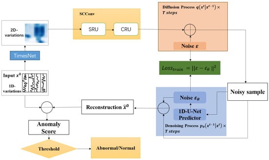
Figure 1.
Framework of SDADT.
3.1. TimesNet
In time series analysis, periodicity (or seasonality) is a prominent feature of the data, particularly in application scenarios with pronounced cyclical fluctuations, such as power demand analysis, sensor data, and other similar contexts. The utilization of periodic features helps improve the modeling accuracy of time series data. Traditional time series models, such as ARIMA and LSTM, can handle some periodicity but often perform poorly when faced with complex or multiple periodic fluctuations. These models typically only capture single or simple cycles, limiting their ability to model more intricate patterns. The periodicity in time series data can exhibit multiple scales, and these cycles may overlap or vary over time. Traditional models struggle to simultaneously capture these multi-scale periodic patterns, as they are typically designed to model simpler or single-cycle behaviors. In contrast, TimesNet views every time point in the time series as reasonably independent. On the one hand, it emphasizes inter-period differences by accounting for overlapping time segments to capture interactions between segments. Conversely, it examines the connections between distinct time points within each segment, emphasizing intra-period variations—differences between neighboring times within the same period. Multi-periodic variations in a 1D time series often overlap, and direct handling of such data may lead to confusion. However, by transforming the data into a 2D tensor, different periods can be clearly separated for individual processing. Once the time series is converted into a 2D tensor, the model can process the data in a manner similar to image processing. This improves the model’s capacity to represent both local and global features by making it easier to employ two-dimensional convolution and other methods to capture intricate spatiotemporal relationships. To achieve the aforementioned effect, TimesNet converts the 1D time series into a 2D tensor, as shown in Figure 2. Time points within a single period are contained in each column, while time points at the same phase over multiple periods are represented by each row.

Figure 2.
The multi-periodicity and temporal two-dimensional variation of a time series.
The aforementioned procedure is integrated into TimesNet’s TimesBlock, which models both kinds of variations efficiently by using a parameter-efficient beginning block. Below is a detailed description of the TimesNet configuration. Examining the time series’ periodicity is essential to accurately capturing and illustrating the temporal differences within and between periods. The Fast Fourier Transform (FFT), represented as , can be applied along the time dimension of the 1D time series to achieve this. Here, T represents the time series’ length, and represents the dimensionality of the input features. Using FFT on the time dimension aids in recognizing periodic patterns in the time series. Here is the procedure:
where represents the amplitude of each frequency component in . The highest k frequencies correspond to the most significant periodic lengths of k in the time series. Considering conjugate symmetry in the frequency domain, we restrict our analysis to frequencies within the range . Equation (1) can be summarized as follows:
As illustrated in Figure 3, the original one-dimensional time series is compressed according to the selected periods. This process can be formally expressed as follows:
where is the procedure that adds zeros to the end of the sequence in order to make sure that divides its length. We obtain a series of 2D tensors by carrying out this operation, where each represents the 2D temporal variations dominated by the period .
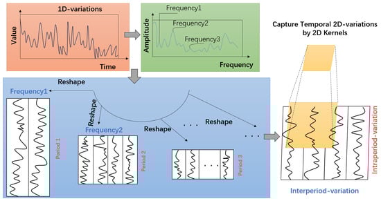
Figure 3.
A univariate example for illustrating the 2D structure in a time series.
TimeBlock
The architecture of TimesNet is shown in Figure 4. In the lth layer of the TimesBlock, the input is , which can be processed using 2D convolution to extract 2D temporal variations. This process can be represented by the following formula:
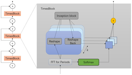
Figure 4.
Framework of TimesNet.
Below is a detailed explanation of the full TimesBlock procedure for collecting the 2D temporal fluctuations of a time series. It mostly consists of the four subprocesses listed below:
- (1)
- Transforming the 1D time series into a 2D tensor.
The first step is to extract and transform the periodicity of the input 1D time feature into a 2D tensor that will represent the 2D temporal fluctuations. The following is a rewrite of the formula based on the previously discussed procedure:
- (2)
- Capturing the 2D temporal variation representation.
We can use 2D convolution to extract information from the 2D tensors with 2D locality . In this case, we use the traditional inception model.
- (3)
- Converting the 2D tensor into a 1D space.
To aggregate the information, we first capture the temporal features and then transform them back into a 1D space.
where indicates the process of eliminating the zeros added during the operation in step (1), and .
- (4)
- Adaptive Aggregation
As in Autoformer [20], the adaptive fusion mechanism generates the final output by performing a weighted sum of the 1D representations obtained according to their corresponding frequency values.
The TimesBlock can record multi-scale and fine-grained 2D temporal patterns at the same time. Thus, TimesNet achieves more efficient representation learning than directly extracting features from a 1D time series.
3.2. DDPMs
A distribution that approximates the initial data distribution of two Markov chain processes is what DDPMs aim to learn. Over a number of steps, noise is gradually added to the input in the forward process. In the opposite procedure, the input is recovered by eliminating the noise that a neural network predicted.
Gaussian noise is gradually injected into the initial input, resulting in a series of latent variables at each diffusion step . Each step is controlled by a noise schedule function , which can be mathematically expressed as
Given , we can sample at any time step in a closed form:
where and .
Starting from , we sample from over T steps to remove the noise until is reconstructed. For a sufficiently small , approximates a Gaussian distribution, and it can be parameterized by the model . This reverse process can be formulated as follows:
According to Bayes’ theorem, the posterior distribution takes the form of
with
We train the neural network to predict at each time step t using as the input. The current diffusion time step is specified by sinusoidal positional embeddings. The training objective can be described as optimizing the negative log-likelihood [21], as follows:
After simplification, the training loss is defined as minimizing:
3.3. SCConv
As shown in Figure 5, the two units that make up SCConv are the Channel Reconstruction Unit (CRU) and the Spatial Reconstruction Unit (SRU). Whereas the CRU reduces channel redundancy by using a segmentation–transformation–fusion strategy, the SRU suppresses spatial redundancy by using a separation–reconstruction approach. Combining SCConv with TimesNet improves performance by cutting down on redundant features, drastically lowering computational cost and complexity, and successfully enhancing anomaly detection performance.
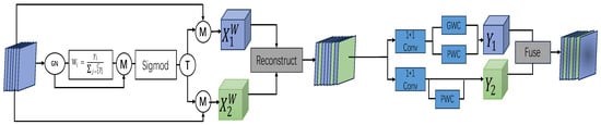
Figure 5.
Framework of SCConv.
For SRU, it utilizes separation and reconstruction operations: First, Group Normalization (GN) is used to normalize the input features [22]. Then, the trainable parameters are re-weighted, and the resulting weights are processed through the function to map them to the range [0, 1]. Weights greater than 0.5 are considered information weights , while the remaining weights are considered non-informative weights . Specifically, as shown in Equation (21):
Subsequently, the input features X are multiplied by and , respectively, resulting in with rich feature information and with redundant information. These two parts then undergo cross-reconstruction operations to obtain spatially refined features. In the case of the CRU, the feature map is initially divided into two channels, and , and is then compressed using a convolution to improve computational efficiency. One set of features serves as a rich feature extractor and undergoes GWC (Group-wise Convolution) with and a operation called PWC (Point-wise Convolution), resulting in a mapping with rich features. This operation enhances the overall feature extraction process and helps reduce computational complexity while maintaining or improving feature richness for anomaly detection tasks. The other set of features uses PWC to extract shallow features, complementing the rich feature extractor, resulting in the mapping . Finally, both and undergo global average pooling to reduce dimensionality and the number of parameters, producing the outputs and . This process is mathematically represented as
Then, through a channel-wise soft attention operation, feature vectors and are obtained. These two feature vectors are used to combine and along the channel dimension, thereby obtaining the channel-refined features. This process is mathematically represented as
3.4. Anomaly Score
The input time series data are passed through the model to generate a reconstructed output, obtaining the predicted reconstruction values. The actual values at each time point are then compared with the reconstructed values, and an anomaly score is calculated. The Mean Squared Error (MSE) formula, which is a measure of the reconstruction error, is used to calculate the anomaly score, as indicated in Equation (25):
where is the actual value, is the reconstructed value, and n is the sequence length.
In this error distribution, most of the normal data points have a small MSE, while anomalous data points typically have a higher MSE. Therefore, the error distribution reflects the normal and anomalous patterns in the data. An anomaly is defined as one where the anomaly score is greater than a predetermined threshold; if the anomaly score is less than the threshold, it is considered normal.
4. Experiment
4.1. Dataset
The SWaT, PSM, SMD, and SMAP are commonly used datasets for anomaly detection in CPSs due to their relevance in real-world industrial and server monitoring applications. SWaT (Secure Water Treatment) focuses on water treatment systems, while the PSM (Prognostics Server Machine) includes predictive maintenance and system management data. The SMD (Server Machine Dataset) provides data on server health and performance. The SMAP (Soil Moisture Active Passive) dataset is a high-resolution, satellite-derived collection of global soil moisture measurements, designed to monitor and analyze terrestrial water cycles. These datasets are particularly valuable because they contain labeled anomalies and reflect the complex, dynamic behaviors typical in industrial and server environments. Table 1 summarizes the statistics of the three datasets, covering server monitoring as well as water treatment applications:

Table 1.
Statistics for the three datasets utilized in the experiments.
- SWaT (Secure Water Treatment) is a CPS cyber security research testbed that replicates an actual industrial water treatment system [23]. Developed by the Singapore University of Technology and Design (SUTD), it aims to study potential cyber attacks and defense measures in critical infrastructure.
- The PSM (Prognostics Server Machine) dataset is a time series dataset for server machine metrics, mainly used for anomaly detection tasks [24]. It was collected by eBay and contains server performance indicators recorded every minute over a period of 21 weeks.
- The SMD (Server Machine Dataset) is designed for multivariate time series anomaly detection [25]. It comprises system performance metrics collected by sensors from servers during their regular operation. This dataset is commonly used in both industry and academia for research related to server anomaly detection.
- The SMAP (Soil Moisture Active Passive) was launched by NASA in January 2015; the SMAP mission combines an L-band radar and radiometer to provide accurate, frequent observations of soil moisture at a spatial resolution of approximately 9 km (radiometer) and 3 km (radar) [26]. The dataset is mainly used for tasks such as remote sensing monitoring and anomaly detection.
4.2. Baselines
We evaluate our suggested approach’s performance against nine well-known anomaly detection models, such as the following:
- LSTM [27]: LSTM is used in anomaly detection by learning normal patterns from time series data. It predicts the next step or reconstructs the input, and anomalies are identified when the prediction or reconstruction error exceeds a predetermined threshold.
- Transformers [28]: Transformers model global dependencies in time series data and identify anomalies by using the self-attention mechanism. Anomalies are identified when the prediction error or reconstruction error of the sequence exceeds a predefined threshold after learning the patterns of normal data.
- LogTrans [29]: LogTrans uses a logarithmic sparse self-attention mechanism to capture time series dependencies both locally and globally. By learning the normal patterns of the data, it performs anomaly detection when the prediction error exceeds a predefined threshold.
- Reformer [30]: To manage a lengthy time series, Reformer employs an effective locality-sensitive hashing self-attention mechanism. By comparing the difference between the actual and predicted values, it learns the typical patterns of behavior and identifies anomalies.
- Pyraformer [31]: Pyraformer efficiently captures multi-scale dependencies in a time series through its pyramid-structured attention mechanism. This enables the model to identify anomaly patterns when processing a long time series, facilitating effective anomaly detection.
- ETSformer [32]: ETSformer detects anomalies by decomposing the time series into three components: level, trend, and seasonality. Anomalies are identified by recognizing abnormal changes in these components. If certain patterns in the data deviate from the expected level, trend, or seasonal behavior, they are flagged as anomalies, enabling effective anomaly detection.
- LightTS [33]: LightTS captures anomaly patterns in a time series efficiently through its self-attention mechanism and multi-scale modeling.
- Dlinear [34]: Dlinear breaks down time series data into trend and seasonal components in order to identify anomalies. It then applies linear models to process these components separately. By learning the linear relationships within the time series, Dlinear identifies anomaly points that deviate from the normal trend.
- CARLA [35]: CARLA utilizes self-supervised contrastive learning to generate embedding representations of a time series. It maximizes the similarity between normal data and minimizes the difference for anomalous data, thereby enabling effective anomaly detection.
4.3. Evaluation Metrics
We evaluate the performance of SDADT using the most common metrics, including , and :
where and stand for true positives, false negatives, and false positives, respectively.
4.4. Data Preprocessing
To increase robustness and speed up convergence, we clean and normalize the data before training the model. Data normalization is used on both the training and test sets, as shown below:
where represents the ith univariate time series. and represent the maximum and minimum values of , respectively. Both reconstruction-based and prediction-based models are susceptible to anomalous and erratic occurrences in the training set. In order to address this issue, we use Spectral Residual (SR) [36], a cutting-edge univariate anomaly identification technique, to find anomalous timestamps in every time series in the training data. We then complete data cleaning by replacing the values of the anomalous timestamps with the surrounding normal values.
4.5. Experimental Setup
The methods and their variants mentioned in this paper were implemented using CUDA 12.7 and PyTorch 12.1 in Python 3.8, and the system used for the experiments had a 12th Gen Intel® Core™ i5-12400F @ 2.50 GHz CPU and an NVIDIA GeForce RTX 4060 Ti GPU. Following Anomaly Transformer’s preprocessing method, we used a sliding window to segment the dataset into continuous, non-overlapping fragments. In previous research, reconstruction was a traditional task for unsupervised point-wise representation learning, and the standard for anomaly detection was the reconstruction error. We employed MSE as the common anomaly detection criterion for all experiments and only altered the base model for reconstruction in order to provide a fair comparison. Regarding hyperparameters, different datasets corresponded to different parameter settings, as shown in Table 2. Here, k represents the variable in Equation (1), denotes the length of the input time series for the model, and the group number denotes the number of groups (g) for Group-wise Convolution in the SCConv module.
Table 2.
Experiment configuration of SDADT.
4.6. Overall Performance
To compare the performance of different models, this paper adopts the widely used Point Adjustment (PA) strategy [37]. The core of this strategy is to adjust errors or biases in the detection results to reduce false positives or false negatives. Particularly when dealing with time-series data, the point-adjustment strategy can optimize the output of detected points.
This paper compares the proposed method with nine baseline models across three real-world datasets, as shown in Table 3. In all three datasets, SDADT performs better in terms of precision than almost all baselines. In particular, it performs best on SMD and only marginally worse than one baseline on the other two datasets. In terms of recall, although it does not achieve the best results among the baselines, it lags behind the best baseline by an average of only about 3.6%. With the exception of SWaT, where it performs only 0.58% worse than the best baseline, our model offers the best detection performance from the standpoint of the F1-score on the majority of datasets. The F1-score and precision performance are the best in the SMAP dataset, while the recall performance is the second best. The experimental findings verify that adding convolution operations to DDPMs improves performance in terms of F1-score, precision, and recall.
Table 3.
Anomaly detection accuracy in terms of precision (%), recall (%), and F1-score, on four datasets with ground-truth labeled anomalies. The best results are in bold, and the second-best is indicated by underline.
4.7. Ablation Study
To investigate the necessity of each component in our proposed method and ensure fairness in the ablation study, we progressively excluded these components while keeping the same hyperparameter settings to observe how the model performance degraded. Our main modifications include removing the DDPM module (denoted as w/o DDPM), removing the SCConv module (denoted as w/o SCConv), and removing both the DDPM and SCConv modules simultaneously (denoted as w/o DDPM and SCConv). The results are shown in Figure 6. From the observations, the conclusions can be drawn as follows:
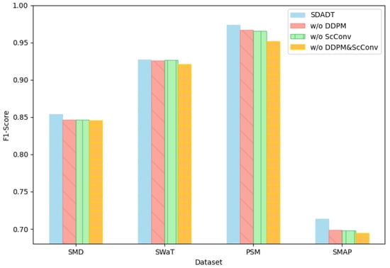
Figure 6.
Comparison of F1-scores in ablation experiments.
When the SCConv module was removed, a significant drop in performance was observed. This phenomenon highlights the importance of capturing feature relevance, and SCConv is capable of capturing multi-scale features. It also demonstrates that the combination of the DDPM module and the convolution module effectively improves experimental performance. The combination shows a more noticeable improvement in the PSM dataset, indicating that it is more effective for anomaly detection in datasets with complex multivariate dependencies, noise, and short-term and long-term features, as well as irregular change patterns.
4.8. Hyperparameter Sensitivity Analysis
To investigate the sensitivity of the model to hyperparameters, this section selects two hyperparameters to study the hyperparameter sensitivity of SDADT.
We introduce the hyperparameter k in Equation (1) to select the most significant frequencies. The parameter k determines the number of frequency components selected, specifically choosing the k components with the highest amplitudes as the primary periodic features of the sequence. Figure 7 illustrates the experimental results of the model under different values of k while keeping other hyperparameters consistent. As shown in the figure, the model consistently maintains stable F1-scores across different datasets. The model’s capacity to learn from the data distribution is improved by the newly introduced DDPM module, which produces samples that roughly reflect the original data distribution through the diffusion process. In the meantime, the expression is enhanced in both spatial and channel dimensions, and feature redundancy is successfully reduced by the SCConv module. The inclusion of these modules makes the model more robust in handling input features, thereby reducing the model’s sensitivity to the hyperparameter k.
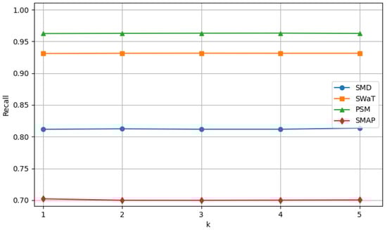
Figure 7.
Performance of F1-score with varying k values.
Image_size is an important parameter in DDPMs for adjusting the reconstructed image size. Figure 8 shows that both excessively large and small values of image_size negatively affect the performance of anomaly detection. This indicates that when the image_size is too small, the representation of the data after converting them into a 2D tensor may be overly compact, leading to the insufficient representation of some important time series features. For example, some long-period fluctuations or trend information may be compressed or lost in tensors with small sizes, making it difficult for the model to capture the full patterns in the data, thereby affecting the accuracy of anomaly detection. As the image_size increases, it significantly raises computational costs and model complexity. This can lead to excessively long training times, higher memory requirements, and even issues such as gradient vanishing or explosion, ultimately affecting the model’s training performance and stability.
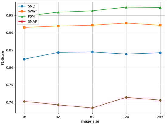
Figure 8.
Performance of F1-score with varying image_size values.
As shown in Figure 9, the optimal seq_len is inherently tied to the temporal scale of anomalies and the trade-off between context integration and noise suppression. Adaptive seq_len selection is guided by anomaly duration.Future work could explore dynamic sequence length tuning based on real-time anomaly characteristics.
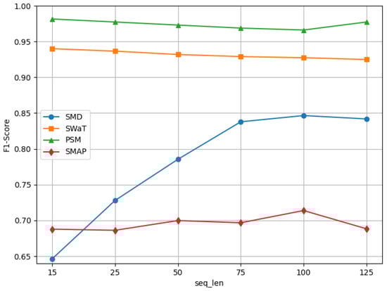
Figure 9.
Performance of F1-score with varying seq_len values.
5. Conclusions
In this study, we innovatively combined TimesNet, DDPM, and SCConv to construct a novel model architecture for anomaly detection. We compared this model with a variety of sophisticated baseline models and thoroughly assessed its performance in anomaly detection tasks using rigorous and extensive experiments on several publicly available datasets. The experimental findings clearly show that the suggested model performs noticeably better in anomaly detection. In particular, it outperforms baseline models in important performance metrics like precision, recall, and F1-score. The findings of this study provide a new and effective solution for anomaly detection, which is expected to play an important role in practical applications. However, our research also has certain limitations. For example, the model may face challenges related to computational resources and time costs when handling extremely large datasets. Due to the large number of features in large datasets, it is difficult to quickly and accurately obtain features, resulting in longer training time. We may be looking for new methods to enhance the feature extraction module. In addition, the model’s performance can still be enhanced for data with unique distributions or noise features. In future work, we intend to further optimize the model architecture, investigate more efficient algorithms to improve computational efficiency, and investigate how to improve the model’s adaptability to complex data environments, all with the goal of improving its performance in anomaly detection tasks.
Author Contributions
Conceptualization, J.Z.; Methodology, J.Z.; Software, J.Z.; Validation, X.Y.; Writing—original draft, J.Z.; Funding acquisition, Z.R. All authors have read and agreed to the published version of the manuscript.
Funding
This research was funded by Key R&D Program of Zhejiang Province, grant number 2023C01023, 2024C01134.
Data Availability Statement
Data are contained within the article.
Conflicts of Interest
The authors declare no conflicts of interest.
Abbreviations
The following abbreviations are used in this manuscript:
| CPSs | Cyber Physical Systems |
| SCConv | Spatial and Channel Reconstruction Convolution |
| DDPMs | Denoising Diffusion Probabilistic Models |
| FFT | Fast Fourier Transform |
| SRU | Spatial Reconstruction Unit |
| CRU | Channel Reconstruction Unit |
| GN | Group Normalization |
| GWC | Group-wise Convolution |
| PWC | Point-wise Convolution |
| MSE | Mean Squared Error |
| SWaT | Secure Water Treatment |
| PSM | Prognostics Server Machine |
| SMD | Server Machine Dataset |
| SMAP | Soil Moisture Active Passive |
| PA | Point Adjustment |
| SR | Spectral Residual |
References
- Deng, A.; Hooi, B. Graph neural network-based anomaly detection in multivariate time series. In Proceedings of the AAAI Conference on Artificial Intelligence, Virtual Event, 2–9 February 2021; Volume 35, pp. 4027–4035. [Google Scholar]
- Ogie, R.I. Cyber security incidents on critical infrastructure and industrial networks. In Proceedings of the 9th International Conference on Computer and Automation Engineering, Sydney, Australia, 18–21 February 2017; pp. 254–258. [Google Scholar]
- Zhai, L.; Vamvoudakis, K.G. A data-based private learning framework for enhanced security against replay attacks in cyber-physical systems. Int. J. Robust Nonlinear Control 2021, 31, 1817–1833. [Google Scholar] [CrossRef]
- Zamanzadeh Darban, Z.; Webb, G.I.; Pan, S.; Aggarwal, C.; Salehi, M. Deep learning for time series anomaly detection: A survey. ACM Comput. Surv. 2024, 57, 1–42. [Google Scholar] [CrossRef]
- Canizo, M.; Triguero, I.; Conde, A.; Onieva, E. Multi-head CNN–RNN for multi-time series anomaly detection: An industrial case study. Neurocomputing 2019, 363, 246–260. [Google Scholar] [CrossRef]
- Kim, J.; Kang, H.; Kang, P. Time-series anomaly detection with stacked Transformer representations and 1D convolutional network. Eng. Appl. Artif. Intell. 2023, 120, 105964. [Google Scholar] [CrossRef]
- Wu, H.; Hu, T.; Liu, Y.; Zhou, H.; Wang, J.; Long, M. Timesnet: Temporal 2d-variation modeling for general time series analysis. arXiv 2022, arXiv:2210.02186. [Google Scholar]
- Gaba, S.; Budhiraja, I.; Kumar, V.; Martha, S.; Khurmi, J.; Singh, A.; Singh, K.K.; Askar, S.S.; Abouhawwash, M. A systematic analysis of enhancing cyber security using deep learning for cyber physical systems. IEEE Access 2024, 12, 6017–6035. [Google Scholar] [CrossRef]
- Rigatos, G.; Zervos, N.; Serpanos, D.; Siadimas, V.; Siano, P.; Abbaszadeh, M. Fault diagnosis of gas-turbine power units with the Derivative-free nonlinear Kalman Filter. Electr. Power Syst. Res. 2019, 174, 105810. [Google Scholar] [CrossRef]
- Hao, W.; Yang, T.; Yang, Q. Hybrid statistical-machine learning for real-time anomaly detection in industrial cyber–physical systems. IEEE Trans. Autom. Sci. Eng. 2021, 20, 32–46. [Google Scholar] [CrossRef]
- de Araujo-Filho, P.F.; Kaddoum, G.; Campelo, D.R.; Santos, A.G.; Macêdo, D.; Zanchettin, C. Intrusion detection for cyber–physical systems using generative adversarial networks in fog environment. IEEE Internet Things J. 2020, 8, 6247–6256. [Google Scholar] [CrossRef]
- Pang, G.; Shen, C.; Cao, L.; Hengel, A.V.D. Deep learning for anomaly detection: A review. ACM Comput. Surv. (CSUR) 2021, 54, 1–38. [Google Scholar] [CrossRef]
- Zhou, X.; Liang, W.; Shimizu, S.; Ma, J.; Jin, Q. Siamese neural network based few-shot learning for anomaly detection in industrial cyber-physical systems. IEEE Trans. Ind. Inform. 2020, 17, 5790–5798. [Google Scholar] [CrossRef]
- Akowuah, F.; Kong, F. Real-time adaptive sensor attack detection in autonomous cyber-physical systems. In Proceedings of the 2021 IEEE 27th Real-Time and Embedded Technology and Applications Symposium (RTAS), Nashville, TN, USA, 18–21 May 2021; IEEE: Piscataway, NJ, USA, 2021; pp. 237–250. [Google Scholar]
- Li, J.; Wen, Y.; He, L. Scconv: Spatial and channel reconstruction convolution for feature redundancy. In Proceedings of the IEEE/CVF Conference on Computer Vision and Pattern Recognition, Vancouver, BC, Canada, 17–24 June 2023; pp. 6153–6162. [Google Scholar]
- Li, G.; Jung, J.J. Deep learning for anomaly detection in multivariate time series: Approaches, applications, and challenges. Inf. Fusion 2023, 91, 93–102. [Google Scholar] [CrossRef]
- Jiang, W.; Hong, Y.; Zhou, B.; He, X.; Cheng, C. A GAN-based anomaly detection approach for imbalanced industrial time series. IEEE Access 2019, 7, 143608–143619. [Google Scholar] [CrossRef]
- Niu, Z.; Yu, K.; Wu, X. LSTM-based VAE-GAN for time-series anomaly detection. Sensors 2020, 20, 3738. [Google Scholar] [CrossRef] [PubMed]
- Wyatt, J.; Leach, A.; Schmon, S.M.; Willcocks, C.G. Anoddpm: Anomaly detection with denoising diffusion probabilistic models using simplex noise. In Proceedings of the IEEE/CVF Conference on Computer Vision and Pattern Recognition, New Orleans, LA, USA, 18–24 June 2022; pp. 650–656. [Google Scholar]
- Wu, H.; Xu, J.; Wang, J.; Long, M. Autoformer: Decomposition transformers with auto-correlation for long-term series forecasting. Adv. Neural Inf. Process. Syst. 2021, 34, 22419–22430. [Google Scholar]
- Sohl-Dickstein, J.; Weiss, E.; Maheswaranathan, N.; Ganguli, S. Deep unsupervised learning using nonequilibrium thermodynamics. In Proceedings of the International Conference on Machine Learning, PMLR, Lille, France, 7–9 July 2015; pp. 2256–2265. [Google Scholar]
- Wu, Y.; He, K. Group normalization. In Proceedings of the European Conference on Computer Vision (ECCV), Munich, Germany, 8–14 September 2018; pp. 3–19. [Google Scholar]
- Mathur, A.P.; Tippenhauer, N.O. SWaT: A water treatment testbed for research and training on ICS security. In Proceedings of the 2016 International Workshop on Cyber-Physical Systems for Smart Water Networks (CySWater), Vienna, Austria, 11 April 2016; IEEE: Piscataway, NJ, USA, 2016; pp. 31–36. [Google Scholar]
- Abdulaal, A.; Liu, Z.; Lancewicki, T. Practical approach to asynchronous multivariate time series anomaly detection and localization. In Proceedings of the 27th ACM SIGKDD Conference on Knowledge Discovery & Data Mining, Singapore, 14–18 August 2021; pp. 2485–2494. [Google Scholar]
- Su, Y.; Zhao, Y.; Niu, C.; Liu, R.; Sun, W.; Pei, D. Robust anomaly detection for multivariate time series through stochastic recurrent neural network. In Proceedings of the 25th ACM SIGKDD International Conference on Knowledge Discovery & Data Mining, Anchorage, AK, USA, 4–8 August 2019; pp. 2828–2837. [Google Scholar]
- Zhao, H.; Wang, Y.; Duan, J.; Huang, C.; Cao, D.; Tong, Y.; Xu, B.; Bai, J.; Tong, J.; Zhang, Q. Multivariate time-series anomaly detection via graph attention network. In Proceedings of the 2020 IEEE International Conference on Data Mining (ICDM), Sorrento, Italy, 17–20 November 2020; IEEE: Piscataway, NJ, USA, 2020; pp. 841–850. [Google Scholar]
- Hochreiter, S. Long Short-term Memory. Neural Comput. 1997, 9, 1735–1780. [Google Scholar] [CrossRef]
- Vaswani, A. Attention is all you need. Adv. Neural Inf. Process. Syst. 2017. [Google Scholar]
- Li, S.; Jin, X.; Xuan, Y.; Zhou, X.; Chen, W.; Wang, Y.X.; Yan, X. Enhancing the locality and breaking the memory bottleneck of transformer on time series forecasting. Adv. Neural Inf. Process. Syst. 2019, 32. [Google Scholar]
- Kitaev, N.; Kaiser, Ł.; Levskaya, A. Reformer: The efficient transformer. arXiv 2020, arXiv:2001.04451. [Google Scholar]
- Liu, S.; Yu, H.; Liao, C.; Li, J.; Lin, W.; Liu, A.X.; Dustdar, S. Pyraformer: Low-Complexity Pyramidal Attention for Long-Range Time Series Modeling and Forecasting. 2022. Available online: https://openreview.net/forum?id=0EXmFzUn5I (accessed on 10 February 2025).
- Woo, G.; Liu, C.; Sahoo, D.; Kumar, A.; Hoi, S. Etsformer: Exponential smoothing transformers for time-series forecasting. arXiv 2022, arXiv:2202.01381. [Google Scholar]
- Zhang, T.; Zhang, Y.; Cao, W.; Bian, J.; Yi, X.; Zheng, S.; Li, J. Less is more: Fast multivariate time series forecasting with light sampling-oriented mlp structures. arXiv 2022, arXiv:2207.01186. [Google Scholar]
- Zeng, A.; Chen, M.; Zhang, L.; Xu, Q. Are transformers effective for time series forecasting? In Proceedings of the AAAI Conference on Artificial Intelligence, Washington, DC, USA, 7–14 February 2023; Volume 37, pp. 11121–11128. [Google Scholar]
- Darban, Z.Z.; Webb, G.I.; Pan, S.; Aggarwal, C.C.; Salehi, M. CARLA: Self-supervised contrastive representation learning for time series anomaly detection. Pattern Recognit. 2025, 157, 110874. [Google Scholar] [CrossRef]
- Ren, H.; Xu, B.; Wang, Y.; Yi, C.; Huang, C.; Kou, X.; Xing, T.; Yang, M.; Tong, J.; Zhang, Q. Time-series anomaly detection service at microsoft. In Proceedings of the 25th ACM SIGKDD International Conference on Knowledge Discovery & Data Mining, Anchorage, AK, USA, 4–8 August 2019; pp. 3009–3017. [Google Scholar]
- Xu, H.; Chen, W.; Zhao, N.; Li, Z.; Bu, J.; Li, Z.; Liu, Y.; Zhao, Y.; Pei, D.; Feng, Y.; et al. Unsupervised anomaly detection via variational auto-encoder for seasonal kpis in web applications. In Proceedings of the 2018 World Wide Web Conference, Lyon, France, 23–27 April 2018; pp. 187–196. [Google Scholar]
Disclaimer/Publisher’s Note: The statements, opinions and data contained in all publications are solely those of the individual author(s) and contributor(s) and not of MDPI and/or the editor(s). MDPI and/or the editor(s) disclaim responsibility for any injury to people or property resulting from any ideas, methods, instructions or products referred to in the content. |
© 2025 by the authors. Licensee MDPI, Basel, Switzerland. This article is an open access article distributed under the terms and conditions of the Creative Commons Attribution (CC BY) license (https://creativecommons.org/licenses/by/4.0/).