FPGA Implementation of Image Encryption by Adopting New Shimizu–Morioka System-Based Chaos Synchronization

Abstract

This study presents an innovative approach utilizing the new Shimizu–Morioka chaotic system. By integrating adaptive backstepping control with GYC partial region stability theory, we successfully achieve synchronization of a slave system with the proposed Shimizu–Morioka chaotic system. The architecture, encompassing the chaotic master system, synchronized slave system, adaptive backstepping controllers, and parameter update laws, has been implemented on an FPGA platform. Comparative analysis demonstrates that the synchronization convergence times (e1, e2, e3, and e4) are significantly reduced compared to conventional adaptive backstepping control methods, exhibiting speed enhancements of approximately 3.42, 3.55, 5.89, and 9.23 times for e1, e2, e3, and e4, respectively. Furthermore, the synchronization results obtained from continuous-time, discrete-time systems, and FPGA implementations exhibit consistent outcomes, validating the effectiveness of the proposed model and controller. Leveraging this validated synchronization framework, chaotic synchronization and secure image encryption are successfully implemented on the FPGA platform. The chaotic signal circuits are meticulously designed and integrated into the FPGA to facilitate a robust image encryption algorithm. In this system, digital signals generated by the synchronized slave chaotic system are utilized for image decryption, while the master chaotic system’s digital signals are employed for encryption. This dual-system architecture highlights the efficacy of the chaotic synchronization method based on the novel Shimizu–Morioka system for practical applications in secure communication.

1. Introduction

With the increasing adoption of mobile devices, the volume of mobile data has surged correspondingly. Among various types of mobile content, video content stands out due to its significantly higher bit rates, making it a primary driver of mobile traffic growth as projected for 2018. The annual growth in mobile video traffic per month is detailed in Ref. [1]. Since a large number of Internet video services fall within the realm of cloud-based applications, the trends in mobile cloud traffic closely mirror those of video content traffic. Despite the inherent memory and processing speed constraints of mobile devices, cloud services such as Netflix, YouTube, Pandora, and Spotify empower users to circumvent these limitations, delivering a seamless media consumption experience regardless of device capability.

Computer networks are inherently vulnerable to a wide range of security threats and attacks. For instance, unauthorized remote access by hackers can lead to data breaches and information compromise. Furthermore, malicious software can potentially erase data across numerous systems, causing substantial losses. Personal data, including sensitive images, messages, and videos, are also at risk of being permanently deleted. These pressing concerns underscore the critical need for robust encryption algorithms designed to enhance security and safeguard personal data from unauthorized access and destruction.

A variety of methods have been developed to encrypt messages and ensure secure transmission, yet the application of chaos in encryption represents a relatively recent innovation. Since the 1990s, researchers have identified a profound connection between chaos theory and cryptography [2,3,4,5]. The key distinction lies in their operational domains: cryptographic systems function within a finite field, whereas chaos theory applies to continuous domains. Despite this divergence, both fields exhibit notable parallels. Core principles of chaos theory, such as mixing, sensitivity to initial conditions, and parameter dependence, strongly correspond to cryptographic principles. For example, the mixing property in chaos theory closely mirrors the diffusion process in cryptographic systems [6].

Table 1. Common characteristics between the properties of chaos and cryptography.

Chaotic Systems	Cryptography Algorithms
Phase space: set of real numbers	Phase space: finite set of integer numbers
Iterations	Rounds
Parameters	Keys
Sensitivity to initial conditions and control parameters	Diffusion
Ergodicity	Confusion
Sensitivity to initial conditions/ control parameter	Diffusion with a small change in the plaintext/secret key
Deterministic dynamics	Deterministic pseudo-randomness
Mixing property	Diffusion with a small change in one plain-block of the whole plaintext
Structure complexity	Algorithm (attack) complexity

illustrates the shared attributes and distinctive features of these two fields [7,8,9].

Since Edward Lorenz’s groundbreaking discovery of a chaotic system [10], numerous chaotic systems have been identified worldwide. Chaos is now recognized as an unpredictable and pervasive phenomenon in nature. Chaos theory has proven to be highly applicable across diverse domains, including digital communication, electronic engineering, biological systems, and secure communication [11,12,13,14,15,16,17,18]. Due to its unique and inherently unpredictable dynamic behavior, chaos presents significant challenges for analysis. As a result, the study of chaotic control and synchronization has garnered substantial attention in both theoretical research and practical applications.

This study proposes an innovative chaotic synchronization framework leveraging adaptive backstepping control and the GYC partial region stability theory [19]. This efficient strategy employs a control Lyapunov function formulated as a simple linear homogeneous function of the system states. As a result, the derived controllers and parameter update laws are substantially simplified, effectively reducing computational overhead and mitigating simulation inaccuracies. The synchronized chaotic systems, comprising the master system, slave system, adaptive backstepping controllers, and parameter update laws, have been successfully implemented on an FPGA platform.

The structure of this paper is as follows: Section 2 provides an overview of the Shimizu–Morioka chaotic system. Section 3 presents an innovative chaos synchronization approach leveraging adaptive backstepping control and the GYC partial region stability theory. The stability of the error dynamic system and the parametric error system is validated using Lyapunov theory, with the update laws derived in this section. Section 4 explores the discretization and FPGA-based implementation of chaos synchronization for the new Shimizu–Morioka system. Section 5 conducts a comprehensive security analysis of the system, highlighting its encryption speed and performance. Furthermore, it demonstrates the practicality of this approach through an FPGA hardware implementation for image encryption and decryption. Finally, Section 6 concludes the paper with key findings and insights.

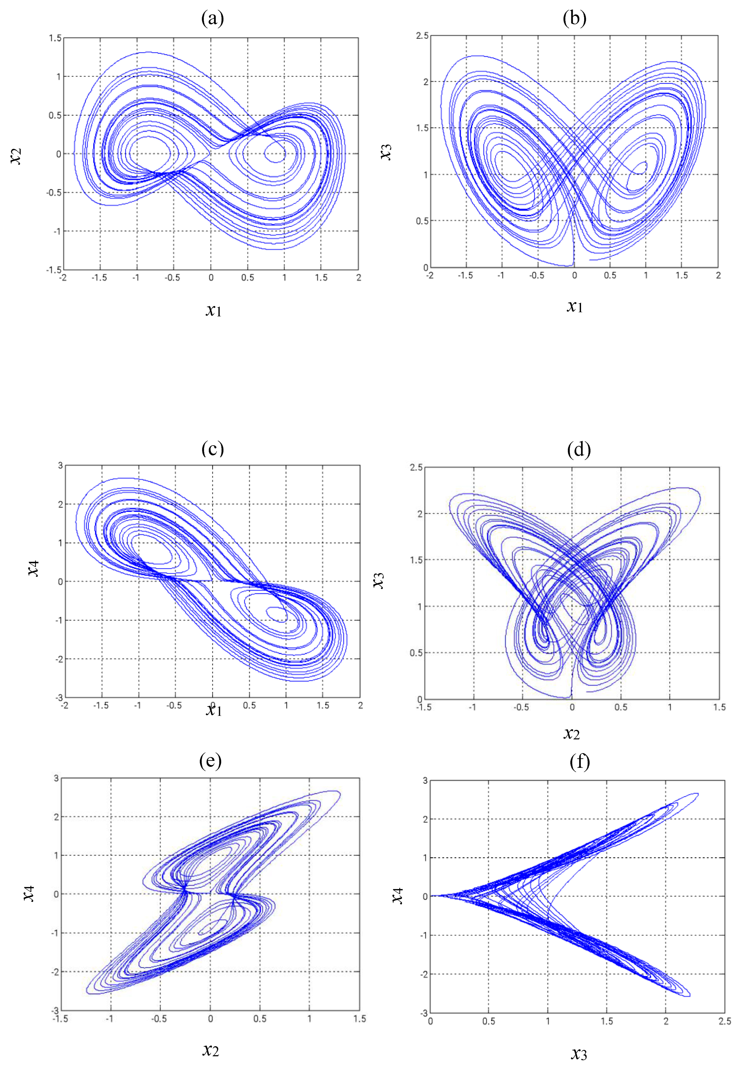
2. Nonlinear Dynamics Analysis of the New Shimizu–Morioka System

The Shimizu–Morioka system is described by the following set of nonlinear differential equations: [20]:

$$\left\{\begin{array}{l}{\dot{x}}_1=x_2\\ {\dot{x}}_2=x_1-b{x}_2-x_1{x}_3\\ {\dot{x}}_3=-a{x}_3+x_1^2\end{array}\right.$$

(1)

The third item of Equation (1) changes ${\dot{x}}_3=-a{x}_3+x_1^2$ to ${\dot{x}}_3=-a{x}_3+r{x}_1^2+d{x}_4$, and adds a fourth item ${\dot{x}}_4=-x_1{x}_3-c{x}_4$ to the four-wing Shimizu–Morioka system, transforming it into a new nonlinear dimensional system. This updated Shimizu–Morioka system is expressed as follows:

$$\left\{\begin{array}{l}{\dot{x}}_1=x_2\\ {\dot{x}}_2=x_1-b{x}_2-x_1{x}_3\\ {\dot{x}}_3=-a{x}_3+r{x}_1^2+d{x}_4\\ {\dot{x}}_4=-x_1{x}_3-c{x}_4\end{array}\right.$$

(2)

In this context, a, b, c, d, and r represent the parameters. For this section, the chosen values for these parameters are a = 0.45, b = 0.75, c = 1, d = 0.01, and r = 0.55.

Figure 1 illustrates the two-dimensional phase diagrams of the modified Shimizu–Morioka system, which exhibit its chaotic dynamics.

3. Achieving Chaotic Synchronization of the Updated Shimizu–Morioka System Through Adaptive Backstepping Control and GYC Partial Region Stability Theory

3.1. Chaos Synchronization Method

Imagine two identical chaotic dynamical systems, where the master system is defined as follows:

$$\dot{x}=Ax+f(x,\hspace{0.33em}B)$$

(3)

where $x={\left[x_1,x_2,\cdots ,x_n\right]}^T$ represents the state vector; $A={\left[A_1,A_2,\cdots ,A_n\right]}^T$ is an $n\times n$ constant coefficient matrix; f s a nonlinear vector function; and $B={\left[B_1,B_2,\cdots ,B_n\right]}^T$ is a vector of constant coefficients in f.

The slave system is described as follows:

$$\dot{y}=\widehat{A}y+f(y,\hspace{0.33em}\widehat{B})+u(t)$$

(4)

where $y={\left[y_1,y_2,\cdots ,y_n\right]}^T$ represents the state vector; $\widehat{A}$ is an $n\times n$ estimated coefficient matrix; $\widehat{B}$ is a vector of estimated coefficients in f; and $u(t)=[u_1\left(t\right),\hspace{0.33em}{u}_2\left(t\right),\hspace{0.33em}\cdots ,\hspace{0.33em}{u}_n\left(t\right){]}^T$ is the control input vector.

Chaos synchronization is achieved as time approaches infinity, when the error vector tends to zero:

$$\underset{t\to \mathrm{\infty }}{lim}{e}_i=0,\hspace{1em}(i=1,\hspace{0.33em}2,\hspace{0.33em}\hspace{0.33em}3,\hspace{0.33em}\cdots ,\hspace{0.33em}n)$$

(5)

$$\mathrm{where} e=y-x+G_k$$

(6)

The constant Gk is chosen. The inclusion of Gk ensures that the error dynamics remain within the first quadrant at all times. By differentiating Equation (6), the error dynamic equations are obtained as follows:

$${\dot{e}}_i={\dot{y}}_i-{\dot{x}}_i,\hspace{1em}(i=1,\hspace{0.33em}2,\hspace{0.33em}\hspace{0.33em}3,\hspace{0.33em}\cdots ,\hspace{0.33em}n)$$

(7)

$${\dot{e}}_i={\widehat{A}}_i{y}_i-A_i{x}_i+f_i(y,\hspace{0.33em}\widehat{B})-f_i(x,\hspace{0.33em}B)+u_i(t),\hspace{1em}(i=1,\hspace{0.33em}2,\hspace{0.33em}\hspace{0.33em}3,\hspace{0.33em}\cdots ,\hspace{0.33em}n)$$

(8)

Using GYC partial region stability theory, Lyapunov functions of the form of positive definite functions in the first quadrant were chosen:

$$\left\{\begin{array}{l}{V}_1(e_1,\hspace{0.33em}{\tilde{A}}_1,\hspace{0.33em}{\tilde{B}}_1)=e_1+{\tilde{A}}_1+{\tilde{B}}_1\\ V_2(V_1,\hspace{0.33em}{e}_2,\hspace{0.33em}{\tilde{A}}_2,\hspace{0.33em}{\tilde{B}}_2)=V_1+e_2+{\tilde{A}}_2+{\tilde{B}}_2\\ \hspace{1em}⋮\hspace{1em}\hspace{1em}\hspace{1em}\hspace{1em}\hspace{1em}\hspace{1em}\hspace{1em}\hspace{1em}\hspace{1em}⋮\\ V_n(V_{n-1},\hspace{0.33em}{e}_n,\hspace{0.33em}{\tilde{A}}_n,\hspace{0.33em}{\tilde{B}}_n)=V_{n-1}+e_n+{\tilde{A}}_n+{\tilde{B}}_n\end{array}\right.$$

(9)

where ${\tilde{A}}_i=A_i-{\widehat{A}}_i$ and ${\tilde{B}}_i=B_i-{\widehat{B}}_i$. ${\tilde{A}}_i$ and ${\tilde{B}}_i$ must be greater than zero.

The derivative along any trajectory of the system described by the differential equations, including Equation (8) and the parameter update equations for ${\tilde{A}}_i$ and ${\tilde{B}}_i$, are as follows:

$$\left\{\begin{array}{l}{\dot{V}}_1(e_1,\hspace{0.33em}{\tilde{A}}_1,\hspace{0.33em}{\tilde{B}}_1)=[{\widehat{A}}_1{y}_1-A_1{x}_1+{\widehat{B}}_1{f}_1(y)-B_1{f}_1(x)+u_1(t)]+{\dot{\tilde{A}}}_1+{\dot{\tilde{B}}}_1\\ {\dot{V}}_2(V_1,\hspace{0.33em}{e}_2,\hspace{0.33em}{\tilde{A}}_2,\hspace{0.33em}{\tilde{B}}_2)={\dot{V}}_1+[{\widehat{A}}_2{y}_2-A_2{x}_2+{\widehat{B}}_2{f}_2(y)-B_2{f}_2(x)+u_2(t)]+{\dot{\tilde{A}}}_2+{\dot{\tilde{B}}}_2\\ \hspace{1em}\hspace{1em}⋮\hspace{1em}\hspace{1em}\hspace{1em}\hspace{1em}\hspace{1em}\hspace{1em}\hspace{1em}\hspace{1em}\hspace{1em}⋮\\ {\dot{V}}_n(V_{n-1},\hspace{0.33em}{e}_n,\hspace{0.33em}{\tilde{A}}_n,\hspace{0.33em}{\tilde{B}}_n)={\dot{V}}_{n-1}+[{\widehat{A}}_n{y}_n-A_n{x}_n+{\widehat{B}}_n{f}_n(y)-B_n{f}_n(x)+u_n(t)]+{\dot{\tilde{A}}}_n+{\dot{\tilde{B}}}_n\end{array}\right.$$

(10)

where ui(t), ${\dot{\tilde{A}}}_i$, and ${\dot{\tilde{B}}}_i$ are selected so that ${\dot{V}}_i={\sum }_{j=1}^i(C_{1j}{e}_j+C_{2j}{\tilde{A}}_j+C_{3j}{\tilde{B}}_j),\hspace{0.33em}\hspace{0.33em}(i=1,\hspace{0.33em}2,\hspace{0.33em}\hspace{0.33em}3,\hspace{0.33em}\cdots ,\hspace{0.33em}n).$ C1j, C2j, and C3j are negative values. The problem to realize the chaos synchronization between two identical chaotic systems now transforms to another problem on how to designed control laws ui and update laws ${\dot{\tilde{A}}}_i$ and ${\dot{\tilde{B}}}_i$ to make $e_i(t)$, ${\tilde{A}}_i=A_i-{\widehat{A}}_i$ and ${\tilde{B}}_i=B_i-{\widehat{B}}_i$ generally converge to zero with time increasing. The design of adaptive backstepping control, combined with GYC partial region stability theory, is employed to accomplish the desired objective.

This paper presents an example where the error dynamics and parameter dynamics are positioned within the first quadrant of the coordinate plane, leveraging the GYC partial region stability framework. The Lyapunov functions applied are simple linear homogeneous expressions of the states, facilitating the development of lower-order controllers that are more efficient and computationally less intensive compared to traditional methods.

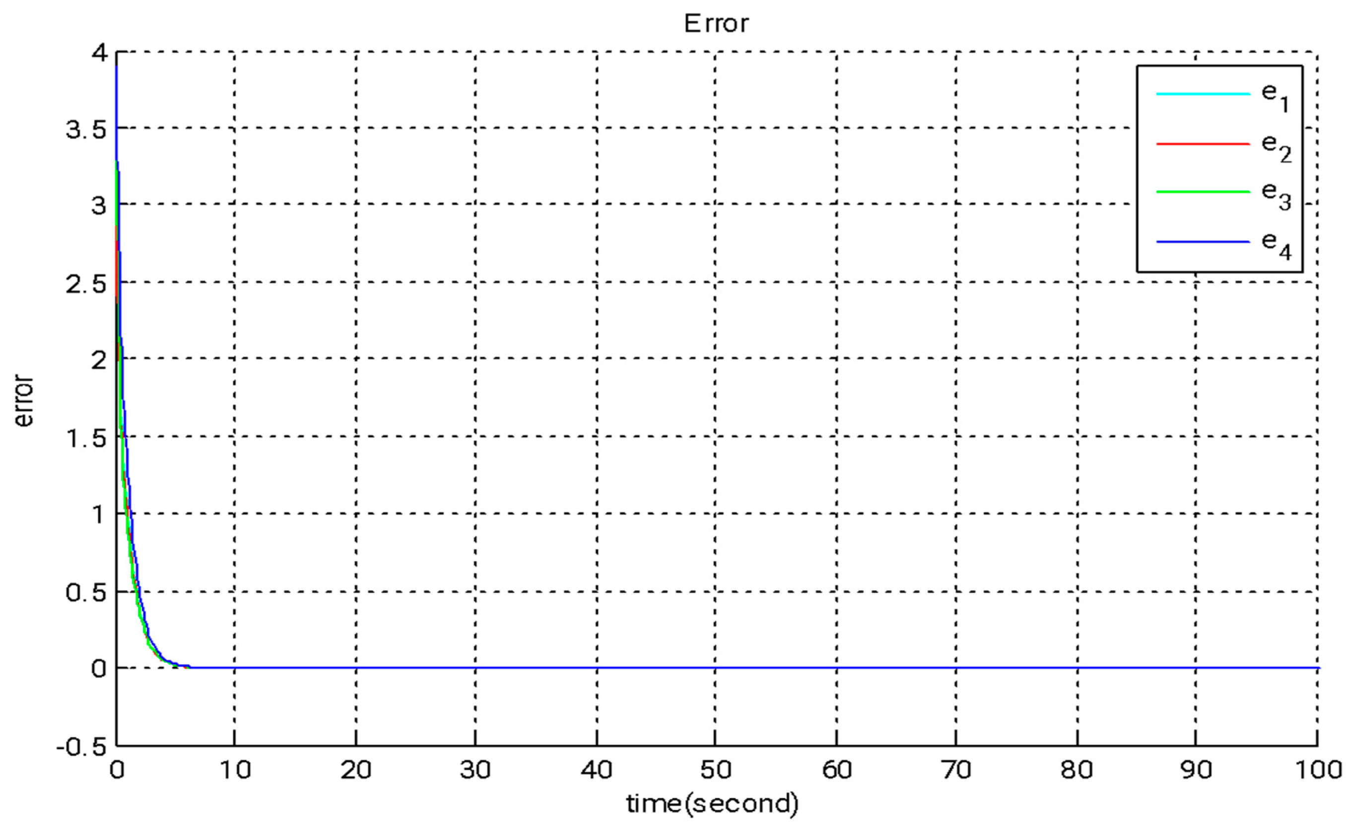
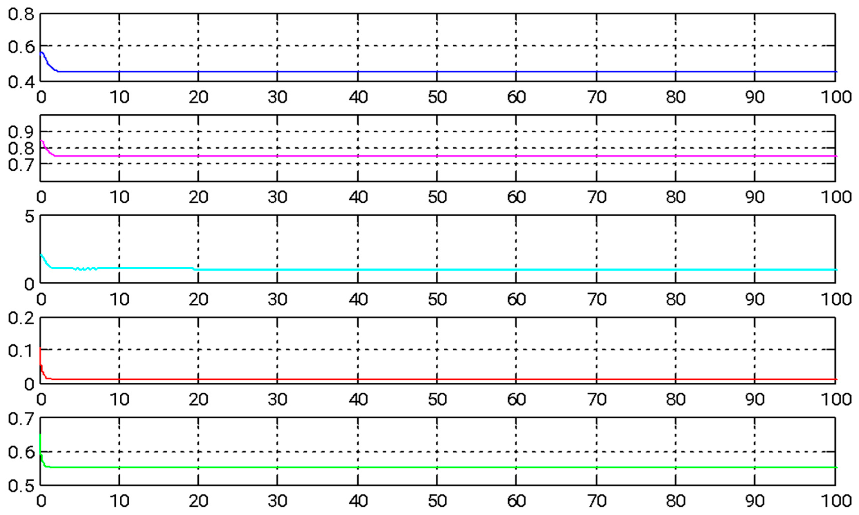
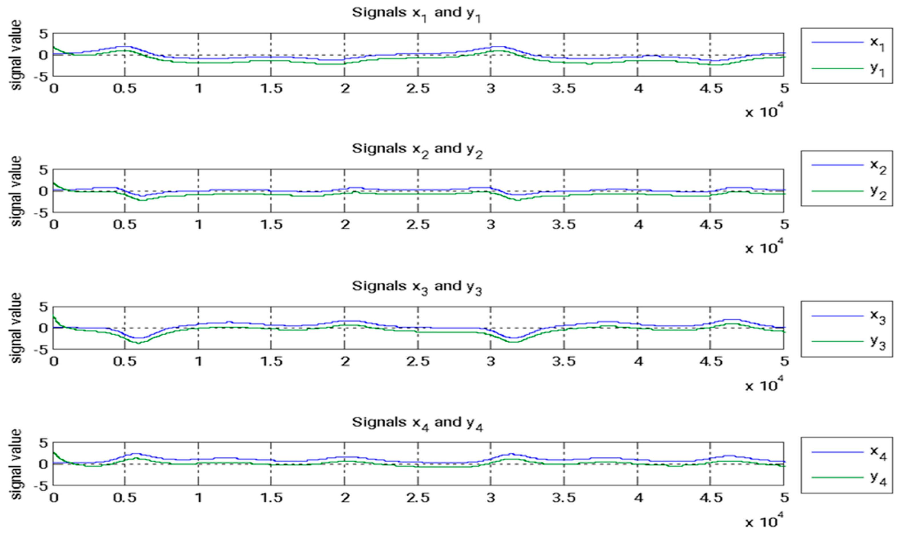
3.2. Design and Numerical Analysis of Synchronization Using Adaptive Backstepping Control with the GYC Partial Region Stability Framework

GYC partial region stability theory [19] is utilized in this section to achieve adaptive backstepping control synchronization. By applying this framework, the new Shimizu–Morioka function can be expressed as a linear homogeneous form, streamlining the controller design process for chaotic synchronization.

This section examines two identical nonlinear dynamical systems, with the slave system tracking and governing the dynamics of the master system. The behavior of the master system is defined by the following set of equations:

$$\left\{\begin{array}{l}{\dot{x}}_1=x_2\\ {\dot{x}}_2=x_1-b{x}_2-x_1{x}_4\\ {\dot{x}}_3=-x_1{x}_4-c{x}_3\\ {\dot{x}}_4=-a{x}_4+r{x}_1^2+d{x}_3\end{array}\right.$$

(11)

where the values of parameters are a = 0.45, b = 0.75, c = 1, d = 0.01, and r = 0.55 in numerical simulation.

The slave system is described as follows:

$$\left\{\begin{array}{l}{\dot{y}}_1=y_2+u_1(t)\\ {\dot{y}}_2=y_1-\widehat{b}{y}_2-y_1{y}_4+u_2(t)\\ {\dot{y}}_3=-y_1{y}_4-\widehat{c}{y}_3+u_3(t)\\ {\dot{y}}_4=-\widehat{a}{y}_4+\widehat{r}{y}_1^2+\widehat{d}{y}_3+u_4(t)\end{array}\right.$$

(12)

The initial conditions of the master system, of the slave system, and of estimated parameters are $x_1=x_2=x_3=x_4=0.1$, $y_1=y_2=2,y_3=y_4=3$, $\widehat{a}=0.55,\hspace{0.33em}\widehat{b}=0.85,\hspace{0.33em}\widehat{c}=2,\hspace{0.33em}\widehat{d}=0.11$, and $\widehat{r}=0.65$, respectively.

The error function can be defined as follows:

$$e_i=y_i-x_i+G_k>0(i=\mathrm{1,2},\mathrm{3,4})$$

(13)

When G_k = 1, inclusion of the constant G_k ensures that the error dynamics always remain in the first quadrant. From the derivative of Equation (13), the error dynamic equation be obtained as follows:

$$\left\{\begin{array}{l}{\dot{e}}_1=(y_2-x_2)+u_1(t)\\ {\dot{e}}_2=(y_1-x_1)-b(y_2-x_2)-\tilde{b}{y}_2-y_1{y}_4+x_1{x}_4+u_2(t)\\ {\dot{e}}_3=-y_1{y}_4+x_1{x}_4-c(y_3-x_3)-\tilde{c}{y}_3+u_3(t)\\ {\dot{e}}_4=-a(y_4-x_4)-\tilde{a}{y}_4+r(y_1^2-x_1^2)+\tilde{r}{y}_1^2+d(y_3-x_3)+\tilde{d}{y}_3+u_4(t)\end{array}\right.$$

(14)

where $\tilde{a}=\widehat{a}-a>0$, $\tilde{b}=\widehat{b}-b>0$, $\tilde{c}=\widehat{c}-c>0$, $\tilde{d}=\widehat{d}-d>0$, and $\tilde{r}=\widehat{r}-r>0$ are the error of parameters, which are positive numbers. u₁(t), u₂(t), u₃(t), and u₄(t) are controllers. These controllers enable the two systems to achieve synchronization as time approaches infinity, with the error function converging to zero in the limit.

Step I. Starting with the first Equation (16), the application of GYC partial region stability theory involves selecting a Lyapunov function (V1), which is a positive definite function specifically defined within the first quadrant:

$$V_1=e_1$$

(15)

The time derivative of this function is expressed as follows:

$${\dot{V}}_1={\dot{e}}_1=(y_2-x_2)+u_1(t)$$

(16)

The controller u₁(t) is defined as follows:

$$u_1(t)=-(y_2-x_2)-e_1)$$

(17)

Equation (16) can be reformulated as follows:

$${\dot{V}}_1=-e_1<0$$

(18)

This function was shown to be a negative definite with respect to e₁ in the first quadrant. As a result, it met the criteria for both the Lyapunov asymptotic stability theorem and the GYC partial region stability framework. The common origin of the error dynamic Equation (16) was determined to be asymptotically stable.

Step II. We consider e₂ to act as the virtual controller.

$$e_2=\alpha e_1=0(\alpha =0)$$

(19)

To analyze the ($e_1$,$m_1$) system, the following was carried out:

According to $e_2=\alpha e_1=0$, m₁ is shown as follows:

$$m_1=e_2-\alpha e_1=e_2$$

(20)

Then, ${\dot{m}}_1$ can be outlined as follows:

$${\dot{m}}_1={\dot{e}}_2=(y_1-x_1)-b(y_2-x_2)-\tilde{b}{y}_2-y_1{y}_4+x_1{x}_4+u_2(t)$$

(21)

Using GYC partial region stability theory, a Lyapunov function (V₂) was chosen as a positive definite function specifically formulated for the first quadrant:

$$V_2=V_1+m_1+\tilde{b}$$

(22)

The time derivative is transformed into the following:

$${\dot{V}}_2={\dot{V}}_1+{\dot{m}}_1+\dot{\tilde{b}}=-e_1+(y_1-x_1)-b(y_2-x_2)-\tilde{b}{y}_2-y_1{y}_4+x_1{x}_4+u_2(t)+\dot{\widehat{b}}$$

(23)

The controller u₂(t) and the parameter update rules ($\dot{\tilde{b}}$) were formulated as follows:

$$u_2(t)=-(y_1-x_1)+b(y_2-x_2)+y_1{y}_4-x_1{x}_4-e_2$$

(24)

$$\dot{\tilde{b}}=\dot{\widehat{b}}=\tilde{b}{y}_2-2\tilde{b}$$

(25)

Equation (23) can be reformulated as follows:

$${\dot{V}}_2=-e_1-e_2-2\tilde{b}<0$$

(26)

This function was shown to be a negative definite with respect to e₁, e₂, and $\tilde{b}$ in the first quadrant. As a result, it adhered to the conditions outlined in both the Lyapunov asymptotic stability theorem and the GYC partial region stability framework. The combined origin of the error dynamics (21) and parameter dynamics (25) was confirmed to exhibit asymptotic stability.

Step III. We designate e₃ as the virtual control input.

$$e_3=\beta e_2=0(\beta )=0$$

(27)

To analyze the ($e_2$,$m_2$) system, the following was carried out:

According to $e_3=\beta e_2=0$, m₂ is shown as follows:

$$m_2=e_3-\beta e_2=e_3$$

(28)

Then, we can represent it as follows:

$${\dot{m}}_2={\dot{e}}_3=-y_1{y}_4+x_1{x}_4-c(y_3-x_3)-\tilde{c}{y}_3+u_3(t)$$

(29)

Using GYC partial region stability theory, a Lyapunov function (V₃) was formulated as a positive definite function, specifically defined for the first quadrant:

$$V_3=V_2+m_2+\tilde{c}$$

(30)

The corresponding time derivative is expressed as follows:

$${\dot{V}}_3={\dot{V}}_2+{\dot{m}}_2+\dot{\tilde{c}}=-(e_1+e_2)-2\tilde{b}-y_1{y}_4+x_1{x}_4-c(y_3-x_3)-\tilde{c}{y}_3+u_3(t)+\dot{\widehat{c}}$$

(31)

The controller u₃(t) and the parameter update law ($\dot{\tilde{c}}$) were developed as follows:

$$u_3(t)=y_1{y}_4-x_1{x}_4+c(y_3-x_3)-e_3$$

(32)

$$\dot{\tilde{c}}=\dot{\widehat{c}}=\tilde{c}{y}_3-2\tilde{c}$$

(33)

Equation (31) can be reformulated in the following manner:

$${\dot{V}}_3=-(e_1+e_2+e_3)-2(\tilde{b}+\tilde{c})<0$$

(34)

This function was confirmed to be a negative definite with respect to e₁, e₂, e₃, $\tilde{b},$ and $\tilde{c}$ within the first quadrant. As a result, it fulfilled the conditions of both the Lyapunov asymptotic stability theorem and the GYC partial region stability framework. The shared origin of the error dynamics (29) and parameter dynamics (33) was determined to exhibit asymptotic stability.

Step IV. Finally, e₄ is designated as the virtual control input.

$$e_4=\gamma e_3=0(\gamma =0)$$

(35)

For studying the ($e_3$,$m_3$) system, the following was carried out:

According to $e_4=\gamma e_3=0$, m₃ is shown as follows:

$$m_3=e_4-\gamma e_3=e_4$$

(36)

Then, we can outline it as follows:

$${\dot{m}}_3={\dot{e}}_4=-a(y_4-x_4)-\tilde{a}{y}_4+r(y_1^2-x_1^2)+\tilde{r}{y}_1^2+d(y_3-x_3)+\tilde{d}{y}_3+u_4(t)$$

(37)

Using the GYC partial region stability theory, a Lyapunov function (V₄) was selected as a positive definite function specifically designed for the first quadrant:

$$V_4=V_3+m_3+\tilde{a}+\tilde{d}+\tilde{r}$$

(38)

The time derivative transforms into the following:

$$\begin{array}{l}{\dot{V}}_4={\dot{V}}_3+{\dot{m}}_3+\dot{\tilde{a}}+\dot{\tilde{d}}+\dot{\tilde{r}}\\ =-(e_1+e_2+e_3)-2(\tilde{b}+\tilde{c})+\dot{\widehat{a}}+\dot{\widehat{d}}+\dot{\widehat{r}}\\ -a(y_4-x_4)-\tilde{a}{y}_4+r(y_1^2-x_1^2)+\tilde{r}{y}_1^2+d(y_3-x_3)+\tilde{d}{y}_3+u_4(t)\end{array}$$

(39)

The controller u₄(t) and update laws of parameters ($\dot{\tilde{a}},\hspace{0.33em}\dot{\tilde{d}},\hspace{0.33em}\mathrm{and}\hspace{0.33em}\dot{\tilde{r}}$) were designed as follows:

$$u_4(t)=a(y_4-x_4)-r(y_1^2-x_1^2)-d(y_3-x_3)-e_4$$

(40)

$$\left\{\begin{array}{l}\dot{\tilde{a}}=\dot{\widehat{a}}=\tilde{a}{y}_4-2\tilde{a}\\ \dot{\tilde{d}}=\dot{\widehat{d}}=-\tilde{d}{y}_3-2\tilde{d}\\ \dot{\tilde{r}}=\dot{\widehat{r}}=-\tilde{r}{y}_1^2-2\tilde{r}\end{array}\right.$$

(41)

Equation (39) can be reformulated as follows:

$${\dot{V}}_4=-(e_1+e_2+e_3+e_4)-2(\tilde{a}+\tilde{b}+\tilde{c}+\tilde{d}+\tilde{r})<0$$

(42)

This function was confirmed to be a negative definite with respect to e₁, e₂, e₃, e₄, $\tilde{a}$, $\tilde{b}$, $\tilde{c}$, $\tilde{d},$ and $\tilde{r}$ in the first quadrant. Consequently, it adhered to both the Lyapunov asymptotic stability theorem and the GYC partial region stability theorem. The shared origin of the error dynamics (37) and parameter dynamics (41) was found to be asymptotically stable.

In this section, we introduce a novel method that combines adaptive backstepping control with the GYC partial region stability theory to accomplish chaos synchronization. This approach provides two major advantages: (I) the Lyapunov functions are formulated as straightforward linear homogeneous functions of system states and update rules; and (II) synchronization performance is greatly enhanced, especially in the context of parameter adaptation. Figure 2, Figure 3 and Figure 4 illustrate the simulation outcomes of the adaptive backstepping control strategy integrated with the GYC partial region stability framework. Figure 5, Figure 6 and Figure 7 display the simulation results of the traditional adaptive backstepping control method.

Table 2. The duration required for error states in a continuous-time system to reach stability.

Method of Control	Error States	e1	e2	e3	e4
Adaptive backstepping control	$\mathbf{e}\le \left|0.1\right|$	t = 18.00 s	t = 16.20 s	t = 16.74 s	t = 17.28 s
	$\mathbf{e}\le \left|0.01\right|$	t = 19.44 s	t = 20.16 s	t = 33.48 s	t = 55.26 s
Adaptive backstepping control with GYC partial region stability theory	$\mathbf{e}\le \left|0.1\right|$	t = 3.533 s	t = 3.366 s	t = 3.366 s	t = 3.700 s
	$\mathbf{e}\le \left|0.01\right|$	t = 5.684 s	t = 5.684 s	t = 5.684 s	t = 5.988 s

provides a comparison of the settling times for the steady-state error between the adaptive backstepping control with the GYC partial region stability theory and the traditional adaptive backstepping control approach.

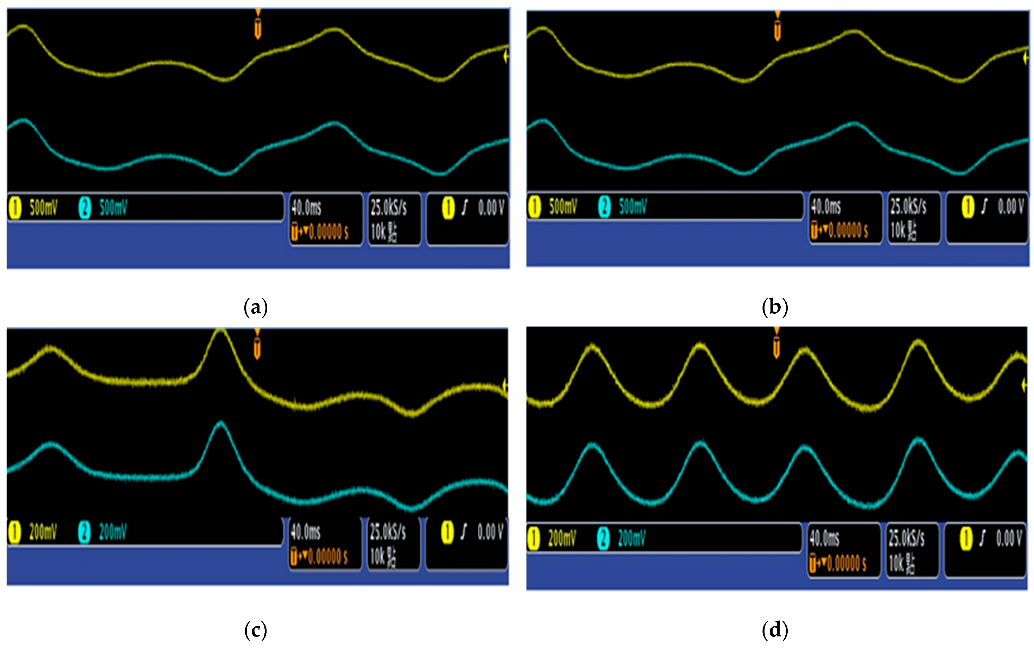
4. The Process of Discretizing the Chaos Synchronization Mechanism for the Updated Shimizu–Morioka System

The master system in continuous time can be represented as follows:

$$\left\{\begin{array}{l}{\dot{x}}_1=x_2\\ {\dot{x}}_2=x_1-b{x}_2-x_1{x}_4\\ {\dot{x}}_3=-x_1{x}_4-c{x}_3\\ {\dot{x}}_4=-a{x}_4+r{x}_1^2+d{x}_3\end{array}\right.$$

(43)

The slave system in continuous time is represented as follows:

$$\left\{\begin{array}{l}{\dot{y}}_1=y_2+u_1(t)\\ {\dot{y}}_2=y_1-\widehat{b}{y}_2-y_1{y}_4+u_2(t)\\ {\dot{y}}_3=-y_1{y}_4-\widehat{c}{y}_3+u_3(t)\\ {\dot{y}}_4=-\widehat{a}{y}_4+\widehat{r}{y}_1^2+\widehat{d}{y}_3+u_4(t)\end{array}\right.$$

(44)

For the numerical simulation, the following parameter values are used: a = 0.45, b = 0.75, c = 1, d = 0.01, and r = 0.55. The starting conditions for both the master and slave systems are as follows: x₁ = x₂ = x₃ = x₄ = 0.1, y₁ = −2, y₂ = 2, y₃ = 3, and y₄ = −3. The initial conditions for the update rule are as follows: $\widehat{a}=0.55,\hspace{0.33em}\widehat{b}=0.85,\hspace{0.33em}\widehat{c}=2,\hspace{0.33em}\widehat{d}=0.11$, and $\widehat{r}=0.65$. These controllers guarantee synchronization between the two systems as time tends toward infinity, with the error function eventually converging to zero. The error function is expressed as follows:

$$e_i=y_i-x_i+G_k>0(i=\mathrm{1,2},\mathrm{3,4})$$

(45)

When G_k = 1, the inclusion of this constant ensures that the error dynamics remain within the first quadrant, thus maintaining positive error states. By differentiating Equation (45), the error dynamic equations can be derived as follows:

$$\left\{\begin{array}{l}{\dot{e}}_1=(y_2-x_2)+u_1(t)\\ {\dot{e}}_2=(y_1-x_1)-b(y_2-x_2)-\tilde{b}{y}_2-y_1{y}_4+x_1{x}_4+u_2(t)\\ {\dot{e}}_3=-y_1{y}_4+x_1{x}_4-c(y_3-x_3)-\tilde{c}{y}_3+u_3(t)\\ {\dot{e}}_4=-a(y_4-x_4)-\tilde{a}{y}_4+r(y_1^2-x_1^2)+\tilde{r}{y}_1^2+d(y_3-x_3)+\tilde{d}{y}_3+u_4(t)\end{array}\right.$$

(46)

where $\tilde{a}=\widehat{a}-a$, $\tilde{b}=\widehat{b}-b$, $\tilde{c}=\widehat{c}-c$, $\tilde{d}=\widehat{d}-d$_, and $\tilde{r}=\widehat{r}-r$. The parameter dynamics must remain positive.

Subsequently, continuous-time Equations (43) and (44) are discretized by using a small sampling interval T, transforming them into their equivalent discrete-time forms.

$$\left\{\begin{array}{l}{x}_1(J)=T[x_2(j)]+x_1(j)\\ x_2(J)=T[x_1(j)-b{x}_2(j)-x_1(j)x_4(j)]+x_2(j)\\ x_3(J)=T[-x_1(j)x_4(j)-c{x}_3(j)]+x_3(j)\\ x_4(J)=T[-a{x}_4(j)+r{x}_1(j)x_1(j)+d{x}_3(j)]+x_4(j)\end{array}\right.$$

(47)

and

$$\left\{\begin{array}{l}{y}_1(J)=T[y_2(j)+u_1(j)]+y_1(j)\\ y_2(J)=T[y_1(j)-\widehat{b}{y}_2(j)-y_1(j)y_4(j)+u_2(j)]+y_2(j)\\ y_3(J)=T[-y_1(j)y_4(j)-\widehat{c}{y}_3(j)+u_3(j)]+y_3(j)\\ y_4(J)=T[-\widehat{a}{y}_4(j)+\widehat{r}{y}_1(j)y_1(j)+\widehat{d}{y}_3(j)+u_4(j)]+y_4(j)\end{array}\right.$$

(48)

where J = kT and j = (k − 1)T, k. The kth time step is represented, with the time step measured in milliseconds. The discrete-time error function can then be expressed as follows:

$$\left\{\begin{array}{l}{e}_1(J)=T[w_2(j)+u_1(j)]+e_1(j)\\ e_2(J)=T[w_1(j)-b{w}_2(j)-\tilde{b}(j)y_2(j)-y_1(j)y_4(j)+x_1(j)x_4(j)+u_2(j)]+e_2(j)\\ e_3(J)=T[-y_1(j)y_4(j)+x_1(j)x_4(j)-c{w}_3(j)-\tilde{c}(j)y_3(j)+u_3(j)]+e_3(j)\\ e_4(J)=T\{-a{w}_4(j)-\tilde{a}(j)y_4(j)+r[y_1(j)y_1(j)-x_1(j)x_1(j)]+\tilde{r}(j)y_1(j)y_1(j)\\ \hspace{1em}\hspace{1em}\hspace{1em}+d{w}_3(j)+\tilde{d}(j)y_3(j)+u_4(j)\}+e_4(j)\end{array}\right.$$

(49)

where $w_i\left(j\right)=y_i\left(j\right)-x_i\left(j\right),(i=\mathrm{1,2},\mathrm{3,4}).$ $\tilde{a}=\widehat{a}-a>0$, $\tilde{b}=\widehat{b}-b>0$, $\tilde{c}=\widehat{c}-c>0$, $\tilde{d}=\widehat{d}-d>0$, and $\tilde{r}=\widehat{r}-r>0.$ These represent errors in the parameters, which are all positive values. u₁(t), u₂(t), u₃(t), and u₄(t) denote the adaptive backstepping controllers, which are formulated as follows:

$$\left\{\begin{array}{l}{u}_1(J)=-w_2(j)-e_1(j)\\ u_2(J)=-w_1(j)+b{w}_2(j)+y_1(j)y_4(j)-x_1(j)x_4(j)-e_2(j)\\ u_3(J)=y_1(j)y_4(j)-x_1(j)x_4(j)+c{w}_3(j)-e_3(j)\\ u_4(J)=a{w}_4(j)-r[y_1(j)y_1(j)-x_1(j)x_1(j)]-d{w}_3(j)-e_4(j)\end{array}\right.$$

(50)

The parameter update rule is selected as follows:

$$\left\{\begin{array}{l}\widehat{a}(J)=T[\tilde{a}(j)y_4(j)-2\tilde{a}(j)]+\widehat{a}(j)\\ \widehat{b}(J)=T[\tilde{b}(j)y_2(j)-2\tilde{b}(j)]+\widehat{b}(j)\\ \widehat{c}(J)=T[\tilde{c}(j)y_3(j)-2\tilde{c}(j)]+\widehat{c}(j)\\ \widehat{d}(J)=T[-\tilde{d}(j)y_3(j)-2\tilde{d}(j)]+\widehat{d}(j)\\ \widehat{r}(J)=T[-\tilde{r}(j)y_1(j)y_1(j)-2\tilde{r}(j)]+\widehat{r}(j)\end{array}\right.$$

(51)

Figure 8 illustrates the state signals for both the master and slave systems. The evolution of the estimated parameters over time is shown in Figure 9. The synchronized waveforms for both systems, captured via FPGA, are presented in Figure 10.

Table 3. The settling time of error states of the discrete time system.

Method of Control	Error States	e1	e2	e3	e4
Adaptive backstepping control	$\mathbf{e}\le \left|0.1\right|$	t = 2.652 s	t = 3.677 s	t = 7.576 s	t = 9.773 s
	$\mathbf{e}\le \left|0.01\right|$	t = 5.911 s	t = 6.988 s	t = 15.378 s	t = 13.644 s
Adaptive backstepping control with GYC partial region stability theory	$\mathbf{e}\le \left|0.1\right|$	t = 3.361 s	t = 3.334 s	t = 3.366 s	t = 3.526 s
	$\mathbf{e}\le \left|0.01\right|$	t = 5.655 s	t = 5.690 s	t = 5.724 s	t = 5.033 s

outlines the settling times for the error states, while

Table 4. The settling time for the error states in the FPGA system.

	Error States	e1	e2	e3	e4
Controllers
Adaptive backstepping		t = 1.858 ms	t = 1.509 ms	t = 1.491 ms	t = 1.480 ms
Adaptive backstepping control with GYC partial region stability theory		t = 1.070 ms	t = 1.467 ms	t = 1.049 ms	t = 1.101 ms

provides the corresponding settling times for the FPGA system. A comparison of the results from Table 3 and Table 4 clearly demonstrates that adaptive backstepping control, enhanced by the GYC partial region stability theory, offers superior performance compared to traditional methods.

5. FPGA-Based Implementation of the Updated Shimizu–Morioka System for Image Encryption

5.1. Research and Method

FPGA is capable of implementing a wide range of circuits, including control systems, chips, and digital signal processing. The circuit is described using VHDL (VHSIC Hardware Description Language) or Verilog HDL (Verilog Hardware Description Language) for simulation, synthesis, and validation. In this chapter, we utilize an Altera DE2-115 development board. The updated Shimizu–Morioka system is compiled for a DE2-115 board using an Altera Cyclone IV 4CE115 chip with VHDL code. The encrypted image is generated using Verilog code. During the practical experiment, a Terasic MTL (Multi-Touch LCD) module is connected to the DE2-115 board to display either the input (GPIO) image or the encrypted image [21,22]. The hardware implementation of the transmitter is carried out using Quartus II. With the RTL Viewer tool in Quartus II, a schematic diagram of the circuit system can be visualized.

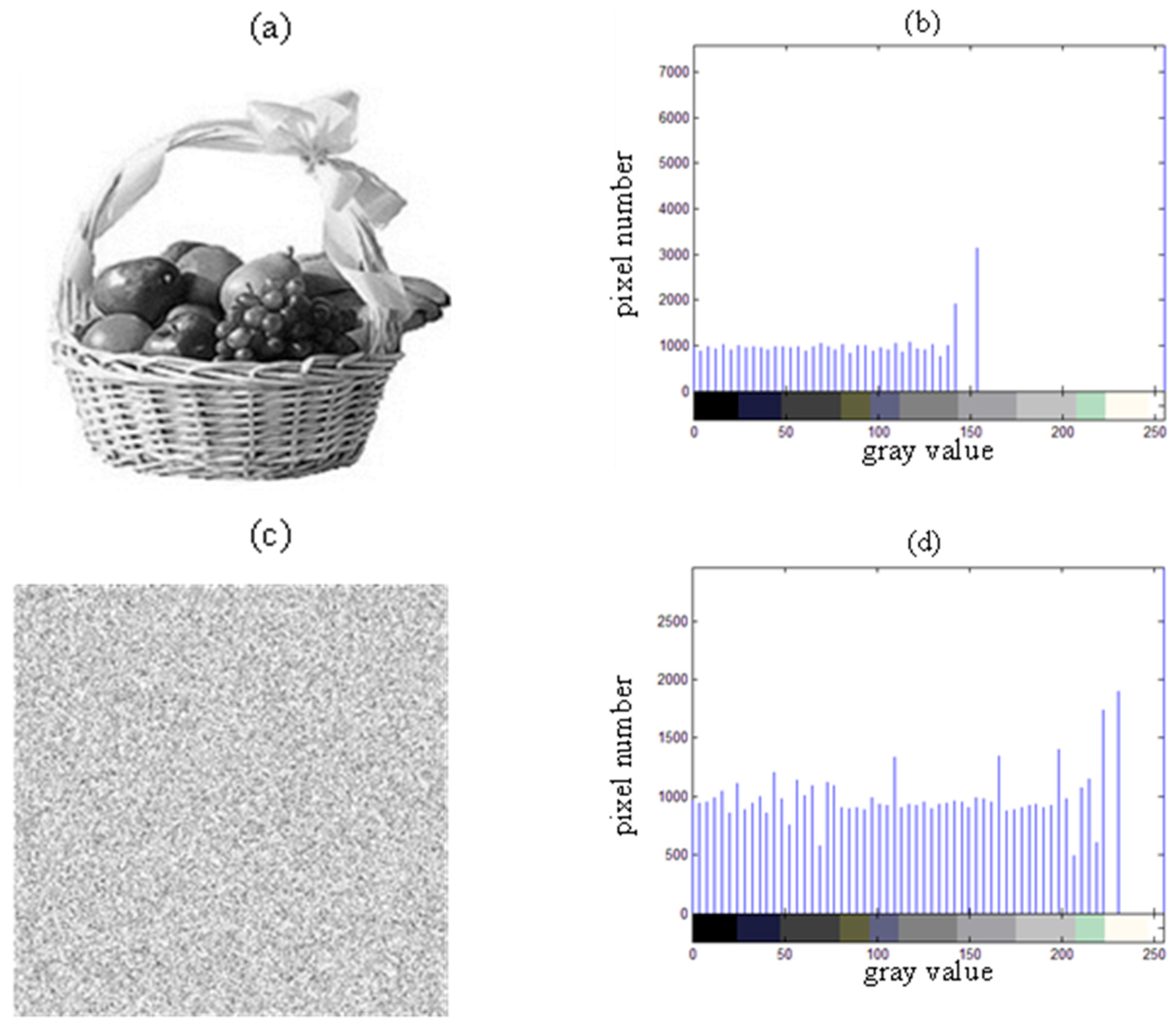
5.2. Image Encryption

In cryptography, the XOR cipher is a basic example of an additive cipher. For example, the string can be 「11101110 00000111」. The string can be encrypted with a cyclic key 「10101111」 in the following manner in

Table 5. Encryption principle of XOR cipher.

Plain text:	11101110	00000111
Encryption key:	10101111	10101111
Cipher text message:	01000001	10101000	The first XOR encryption
Decryption key:	10101111	10101111
Decrypt the message:	11101110	00000111	The second XOR decryption

.

The XOR operation is a key element in many advanced ciphers. However, when utilized with a simple, repeating key, a basic XOR cipher becomes highly susceptible to frequency analysis, making it easy to break. If any part of the message is recognizable or can be guessed, the key is vulnerable. Despite these flaws, the XOR cipher is popular for its ease of implementation and minimal computational demand.

Having understood the XOR encryption technique, we apply it to image encryption in this section. The image has a resolution of 800 × 480 pixels and is in BMP format. To transmit the image, three channels are used for the red (R), green (G), and blue (B) components. Therefore, each pixel consists of 8 × 3 = 24 bits. The total image size is 800 × 480 × 24 = 9,216,000 bits. We can modify each bit of the image by combining it with a chaotic digital signal to achieve encryption. The following are encryption steps:

Step 1: Designing the image output on FPGA.

Step 2: Designing the circuit for the chaotic master system.

Step 3: To integrate these signals together.

Step 4: Producing four distinct signals from the chaotic system (x₁, x₂, x₃, and x₄). Choose x₁, x₂, x₃ to correspond to the color signal (I_R, I_G, I_B) of the original image.

Step 5: Chaotic signal using sort function of sort shift, and converted into $X_1,X_2,X_3$. Let the color gamut signal (I_R, I_G, I_B) correspond to sequence signal ($X_1,X_2,X_3$). Let them use logic operation (XOR) to obtain I_{Mix_R}, I_{Mix_G}, I_{Mix_B}.

Step 6: Finally, output I_{Mix_R}, I_{Mix_G}, I_{Mix_B} to GPIO, and display the encrypted image I_Mix on MTL module.

5.3. Image Decryption

As we have established the synchronization of the new Shimizu–Morioka system in Section 4, we can now use the slave system to decrypt the image encrypted by the master system. The decryption process is illustrated in the flowchart in Figure 11.

The steps for decrypting the image are as follows:

Step 1: Producing four distinct signals from the chaotic system. ($x_5,x_6,x_7$ and $x_8$).

Step 2: We choose $x_5,x_6,x_7$ to correspond to the master chaotic signals ($x_1,x_2,x_3$). Using sort function of sort shift, and converting into $X_5,X_6,X_7$.

Step 3: To integrate these signal sequences.

Step 4: Let the encrypted image color gamut matrix (I_{Mix_R}, I_{Mix_G}, I_{Mix_B}) correspond to the slave system signals ($X_5,X_6,X_7$). Encrypted image signals use sort function of logic operation (XOR). And we can use the XOR truth table and the slave system signals ($X_5,X_6,X_7$) to let every bit be original.

Step 5: Finally, encrypted image color gamut matrix (I_{Mix_R}, I_{Mix_G}, I_{Mix_B}) will be decrypted to the original image (I_R, I_G, I_B).

5.4. Histogram Analysis

A histogram displays how pixel values are distributed across an image. In the case of an encrypted image, the ideal histogram should be uniformly distributed, significantly differing from the original image’s histogram. This ensures that attackers cannot retrieve meaningful statistical data. For our simulation, the test image used is called “Fruit”, with a resolution of 256 × 256 pixels.

Figure 12 demonstrates that the histograms of the encrypted images produced by the algorithm are evenly distributed, which is clearly different from the histogram of the original image. This shows that the encryption effectively masks any relevant information, preventing attackers from utilizing statistical methods to break the cryptosystem.

6. Conclusions

In this study, a novel chaotic system is introduced, extending the Shimizu-Morioka system by incorporating additional parameters and a nonlinear component. By combining GYC partial region stability theory with adaptive backstepping synchronization, we significantly reduce the convergence time of the new chaotic system. The synchronization speeds for e₁, e₂, e₃, and e₄ are found to be approximately 3.42, 3.55, 5.89, and 9.23 times faster, respectively. The synchronization of this complex system is also successfully achieved. Furthermore, the FPGA-based synchronization of the new Shimizu–Morioka system is implemented, with identical results observed across the continuous-time, discrete-time, and FPGA systems. When compared with traditional adaptive backstepping control, the proposed method, using GYC partial region stability theory, outperforms it in performance as presented in Table 2, Table 3 and Table 4. Finally, an image encryption algorithm is developed using FPGA and digital signal processing. Experimental results indicate that the encryption’s key space is sufficiently large to withstand exhaustive key differential attack analysis. The proposed method has been shown to offer robust security, and its processing speed is highly suitable for image encryption tasks. Encryption through logic operations has been completed, and decryption using the slave system has also been successfully achieved, following the implementation of synchronization.

References

1. CISCO. Available online: https://www.cisco.com/#tabs-35d568e0ff-item-194f491212-tab (accessed on 29 January 2025).
2. Brown, R.; Chua, L.O. Clarifying chaos: Examples and counterexamples. Int. J. Bifurc. Chaos 1996, 6, 219–249. [Google Scholar] [CrossRef]
3. Dachselt, F.; Schwarz, W. Chaos and cryptography. IEEE Trans. Circuits Syst. I Fundam. Theory Appl. 2001, 48, 1498–1509. [Google Scholar] [CrossRef]
4. Jakimoski, G.; Kocarev, L. Chaos and cryptography: Block encryption ciphers based on chaotic maps. IEEE Trans. Circuits Syst. I Fundam. Theory Appl. 2001, 48, 163–169. [Google Scholar] [CrossRef]
5. Schmitz, R. Use of chaotic dynamical systems in cryptography. J. Frankl. Inst. 2001, 338, 429–441. [Google Scholar] [CrossRef]
6. Kocarev, L.; Jakimoski, G.; Stojanovski, T.; Parlitz, U. From chaotic maps to encryption schemes. In Proceedings of the 1998 IEEE International Symposium on Circuits and Systems (ISCAS), Monterey, CA, USA, 31 May–3 June 1998; pp. 514–517. [Google Scholar]
7. Alvarez, G.; Li, S. Some basic cryptographic requirements for chaos-based cryptosystems. Int. J. Bifurc. Chaos 2006, 16, 2129–2151. [Google Scholar] [CrossRef]
8. Sankpal, P.R.; Vijaya, P. Image encryption using chaotic maps: A survey. In Proceedings of the 2014 Fifth International Conference on Signal and Image Processing, Bangalore, India, 8–10 January 2014; pp. 102–107. [Google Scholar]
9. Ephin, M.; Joy, J.A.; Vasanthi, N. Survey of Chaos based Image encryption and decryption techniques. In Proceedings of the Amrita International Conference of Women in Computing (AICWIC’13), Coimbatore, India, 9–11 January 2013; International Journal of Computer Applications (IJCA): Wilmington, NC, USA, 2013. [Google Scholar]
10. Lorenz, E.N. Deterministic nonperiodic flow. J. Atmos. Sci. 1963, 20, 130–141. [Google Scholar] [CrossRef]
11. Hsu, W.-T.; Tsai, J.S.-H.; Guo, F.-C.; Guo, S.-M.; Shieh, L.-S. From fault-diagnosis and performance recovery of a controlled system to chaotic secure communication. Int. J. Bifurc. Chaos 2014, 24, 1450151. [Google Scholar] [CrossRef]
12. Mittal, A.; Dwivedi, A.; Dwivedi, S. Parameter adaptation technique for rapid synchronization and secure communication. Eur. Phys. J. Spec. Top. 2014, 223, 1549–1560. [Google Scholar] [CrossRef]
13. Hu, H.; Deng, Y.; Liu, L. Counteracting the dynamical degradation of digital chaos via hybrid control. Commun. Nonlinear Sci. Numer. Simul. 2014, 19, 1970–1984. [Google Scholar] [CrossRef]
14. Liu, S.; Zhang, F. Complex function projective synchronization of complex chaotic system and its applications in secure communication. Nonlinear Dyn. 2014, 76, 1087–1097. [Google Scholar] [CrossRef]
15. Padmanaban, E.; Boccaletti, S.; Dana, S. Emergent hybrid synchronization in coupled chaotic systems. Phys. Rev. E 2015, 91, 022920. [Google Scholar] [CrossRef]
16. Mahmoud, G.M.; Mahmoud, E.E.; Arafa, A.A. Passive control of n-dimensional chaotic complex nonlinear systems. J. Vib. Control 2013, 19, 1061–1071. [Google Scholar] [CrossRef]
17. Hung, M.-L.; Yau, H.-T. Circuit implementation and synchronization control of chaotic horizontal platform systems by wireless sensors. Math. Probl. Eng. 2013, 2013, 903584. [Google Scholar] [CrossRef]
18. Eskov, V.; Gavrilenko, T.; Vokhmina, Y.V.; Zimin, M.; Filatov, M. Measurement of chaotic dynamics for two types of tapping as voluntary movements. Meas. Tech. 2014, 57, 720–724. [Google Scholar] [CrossRef]
19. Ge, Z.-M.; Yu, J.-K.; Chen, H.-K. Three asymptotical stability theorems on partial region with applications. Jpn. J. Appl. Phys. 1998, 37, 2762. [Google Scholar] [CrossRef]
20. El-Dessoky, M.; Yassen, M.; Aly, E. Bifurcation analysis and chaos control in Shimizu–Morioka chaotic system with delayed feedback. Appl. Math. Comput. 2014, 243, 283–297. [Google Scholar] [CrossRef]
21. Tlelo-Cuautle, E.; Carbajal-Gomez, V.; Obeso-Rodelo, P.; Rangel-Magdaleno, J.; Nunez-Perez, J.C. FPGA realization of a chaotic communication system applied to image processing. Nonlinear Dyn. 2015, 82, 1879–1892. [Google Scholar] [CrossRef]
22. Masmoudi, A.; Puech, W. Lossless chaos-based crypto-compression scheme for image protection. IET Image Process. 2014, 8, 671–686. [Google Scholar] [CrossRef]
Figure 1. Phase diagrams of the updated Shimizu–Morioka system: (a)   x 1 - x 2 Phase, (b)   x 1 - x 3 Phase, (c)   x 1 - x 4 Phase, (d)   x 2 - x 3 Phase, (e)   x 2 - x 4 Phase, (f)   x 3 - x 4 Phase.
Electronics 14 00740 g001
Figure 2. State signals of the master and slave systems governed by adaptive backstepping control, incorporating the GYC partial region stability framework.
Electronics 14 00740 g002
Figure 3. The time evolution of error states under adaptive backstepping control utilizing the GYC partial region stability framework.
Electronics 14 00740 g003
Figure 4. The temporal evolution of estimated parameters under adaptive backstepping control employing the GYC partial region stability framework.
Electronics 14 00740 g004
Figure 5. The state signals of the master and slave systems under adaptive backstepping control.
Electronics 14 00740 g005
Figure 6. The temporal progression of error states under adaptive backstepping control.
Electronics 14 00740 g006
Figure 7. The time evolution of estimated parameters during adaptive backstepping control.
Electronics 14 00740 g007
Figure 8. State signals for both the master and slave systems.
Electronics 14 00740 g008
Figure 9. The temporal progression of estimated parameters.
Electronics 14 00740 g009
Figure 10. Actual oscilloscope images of synchronized waveforms for both the master and slave systems, captured using FPGA: (a) y 1 x 1 , (b) y 2 x 2 , (c) y 3 x 3 , and (d) y 4 x 4 .
Electronics 14 00740 g010
Figure 11. A flowchart for encryption and decryption processes.
Electronics 14 00740 g011
Figure 12. (a) The original gray image of Fruit; (b) the histogram of the original grayscale image of Fruit; (c) the grayscale image of Fruit after encryption; and (d) the histogram of the encrypted grayscale image of Fruit.
Electronics 14 00740 g012