Improved Informed RRT*: Based on Dynamic Shrinkage Threshold Node Selection Mechanism and Adaptive Goal-Biased Strategy

Abstract

This study presents an improved Informed RRT* algorithm integrating a dynamic shrinkage threshold node selection mechanism with an adaptive goal-biased strategy, aimed at reducing computational iterations and accelerating convergence performance. To resolve node redundancy during Informed RRT* sampling, a dynamic shrinkage threshold-based node selection mechanism is developed. Through the dynamic evaluation of nodal distances (between newly generated nodes and the existing tree structure) against node selection thresholds, redundant nodes are eliminated to enhance spatial exploration efficiency. To address blind exploration and convergence delays, an adaptive goal-biased strategy guides the directional expansion of the search tree toward target regions, thereby optimizing convergence behavior. Systematic simulations demonstrate the effectiveness of the proposed algorithm across multiple scenarios. Comparative experiments demonstrate that the two key technologies significantly improved the speed of the initial-path generation of Informed RRT*. Moreover, the proposed method shows good adaptability and stability in different environments, which proves its potential and advantages in the path-planning field.

1. Introduction

Advancements in robotics, sensor systems, and computational technologies have driven the expanding adoption of autonomous wheeled mobile robots across the industrial [1], agricultural [2,3], logistics [4], service [5], and autonomous vehicle [6] sectors. Path planning and trajectory tracking have emerged as fundamental enabling technologies for autonomous navigation systems, as demonstrated in recent studies [7].

Contemporary path-planning methodologies can be classified into three primary categories: (1) search-based approaches, comprising Dijkstra’s algorithm [8] and A [9]; (2) sampling-based techniques, including Rapidly exploring Random Trees (RRT), its optimal variant RRT [10], and the informed version Informed RRT* [11]; and (3) bio-inspired algorithms, such as Genetic Algorithms, Ant Colony Optimization, and the Intelligent Bug Algorithm (IBA) [12]. The Rapidly exploring Random Tree (RRT) algorithm, a foundational sampling-based method first introduced by LaValle (1998), provides probabilistically complete exploration in configuration spaces. Initialized from a root node, the algorithm iteratively extends the search tree through stochastic sampling, achieving progressive space exploration via sequential leaf node additions. Upon detecting the target configuration within the expanding tree, the exploration phase terminates automatically, enabling collision-free path extraction. This methodology eliminates explicit spatial discretization requirements while naturally accommodating both kinematic constraints and high-dimensional configuration spaces. With probabilistically complete guarantees and linear time complexity, the algorithm demonstrates inherent capability in obstacle avoidance and differential constraint satisfaction (including nonholonomic and dynamic systems) without requiring explicit path transformations. These characteristics establish RRT as a preferred solution for robotic motion planning in complex environments.

Recent methodological advancements have substantially enhanced the RRT framework’s path optimization capabilities. Zhao et al. [13] integrated dynamic equilibrium control with RRT for environments containing stochastically distributed obstacles, achieving improved convergence–pathlength trade-offs. Comparative analysis demonstrated the dynamic RRT variant’s superior performance relative to Lower Bound Tree-RRT under identical environmental conditions. Wu et al. [14] developed Fast-RRT to address inherent RRT limitations, including prolonged initial-path discovery phases and suboptimal solution trajectories. Tu’s team [15] introduced a narrow passage-optimized RRT that reduces node exploration density and computational latency in constrained indoor spaces. Yu et al. [16] implemented a dual-tree RRT architecture that simultaneously handles kinodynamic constraints and dynamic obstacle avoidance in vehicular path planning.

The RRT* algorithm demonstrates progressive path optimization capabilities, offering distinct advantages in motion planning applications. However, several limitations persist, including (1) suboptimal convergence rates in complex environments, (2) stochastic node expansion behavior, and (3) computational intensity during path refinement [17]. The integration of RRT with artificial potential field (APF) methodologies has proven effective in crowded environments, simultaneously enhancing path feasibility and convergence characteristics. The APF framework reduces iteration counts through intelligent parent node selection, thereby accelerating convergence rates [18]. Beyond RRT-APF integration for enhanced obstacle avoidance, a directional-biased adaptive sampling strategy has been developed to improve global exploration efficiency and solution quality [19]. The synergistic integration of APF with fuzzy adaptive expansion mechanisms significantly improves RRT*’s convergence properties, demonstrating robust performance in dense operational scenarios [20]. The F-RRT* algorithm employs $FindReachest$ and $CreatNode$ operations for parent node generation and path cost optimization, leveraging triangular inequality principles to enhance solution quality and convergence characteristics [21]. Building upon these advancements, FF-RRT* demonstrates enhanced computational efficiency and convergence rates, extending applicability to increasingly complex environments [22].

While demonstrating efficient optimal path generation, Informed RRT* exhibits constrained convergence rates. To address this limitation, a synergistic integration of particle swarm optimization (PSO) with Informed RRT* yields $RRT$-$PSO$, achieving accelerated convergence during path exploration [23]. A probability-smoothed bidirectional RRT (Bi-RRT) variant has been developed, incorporating kinodynamic constraints and goal-oriented sampling strategies. This dual-directional exploration paradigm reduces computational iterations while enhancing convergence properties, ultimately refining solution optimality [24].

The adaptive Informed RRT* achieves asymptotic convergence to optimal solutions, with subsequent elliptical sampling-based local refinement enhancing solution quality. Experimental validation demonstrates the adaptive Informed RRT*’s capability to generate stable optimal trajectories for robotic navigation in constrained environments [25]. While providing asymptotically optimal paths, Informed RRT* exhibits proximity to obstacles, prompting the development of bidirectional Informed RRT* through dual-tree exploration for enhanced path reliability [26]. Addressing irregular obstacle distributions in orchard environments, the continuous bidirectional Quick-RRT* implements dual-tree node smoothing for enhanced path continuity [27]. In medical applications, Bi-RRT incorporates greedy expansion and start-point repulsion mechanisms to optimize sampling efficiency [28]. Leveraging potential fields and explicit bias sampling, the dynamic Informed Bias RRT*-Connect employs adaptive bias points for precise dual-tree growth guidance [29]. An enhanced Informed RRT* variant integrates greedy heuristics, search space reduction, and Dynamic Window Approach (DWA) integration to simultaneously improve path quality and navigation efficiency [30].

While existing studies have advanced Informed RRT*’s capabilities, persistent challenges remain in convergence acceleration and exploration process optimization for guaranteed path quality. This work presents a synergistic integration of dynamic shrinkage threshold node selection with adaptive goal biasing, enhancing search efficiency and environmental adaptability across diverse operational scenarios. The dynamic threshold mechanism enhances exploration efficiency through computational redundancy reduction, while adaptive goal biasing enables directed tree expansion toward target regions. The main innovations and contributions of the article are summarized as follows:

(i)

A dynamic shrinkage threshold node selection mechanism is employed to improve algorithm efficiency. This mechanism dynamically adjusts the selection threshold based on environmental complexity and eliminates redundant nodes during sampling. Furthermore, the threshold shrinks during iterations to prevent the loss of potentially optimal paths in later stages.

(ii)

An adaptive goal-biased strategy is employed to address the problem of blind sampling in Informed RRT. This strategy dynamically adjusts the goal-bias probability based on the obstacle distribution along the line defined in the algorithm, ensuring efficient exploration in complex environments while accelerating convergence in simpler scenarios.

This paper is organized to systematically present the research methodology and findings as follows: Section 2 establishes the theoretical foundation, introducing fundamental algorithms, defining essential concepts, and detailing the core principles of RRT*, Elliptical Sampling, and Informed RRT*. Section 3 presents the proposed improved Informed RRT* algorithm, with comprehensive technical exposition and innovation analysis. Section 4 delivers extensive simulation results, including comparative performance evaluation and critical parameter analysis. Section 5 focuses on robotic platform validation, demonstrating the algorithm’s practical feasibility through comprehensive experimental evaluation. Section 6 concludes with a synthesis of key findings, highlighting the algorithm’s technical advantages and potential applications.

2. Algorithm Overview

In this section, the definition of motion path planning, related work and background, and other algorithms of the paper such as RRT*and Informed RRT* are introduced.

2.1. Basic Definition

The path-planning problem is formally defined on a configuration space X, where $X_{obs}$ is the obstacle area, $X_{free}=X/X_{obs}$ is the accessible area, $x_{start}ϵX_{free}$ is the initial position, $X_{goal}ϵX_{free}$ is the target area, $x_{goal}$ is the end position, and (X, $x_{start}$, $x_{goal}$) are important parameters. Let a continuous function $\sigma$: [0, 1] →$X_{free}$ denote a feasible obstacle-free path, where $\forall \tau ϵ[0,1],\sigma \left(t\right)ϵX_{free}$, $c_{\sigma }$ is the lenth of the path.

Definition 1. 

Feasible path planning is based on (X, $x_{start}$, $x_{goal}$) to find a collision-free path σ, where $\sigma \left(0\right)=x_{start}$ and $\sigma \left(1\right)=x_{goal}$.

Definition 2. 

Path optimization is based on (X, $x_{start}$, $x_{goal}$) to find an optimized path ${\sigma }^{*}$ that minimizes the cost $c\left({\sigma }^{*}\right)$ = min c(σ): σ, where $c\left(\sigma \right)$ is the cost to arrive at $x_{goal}$ along with the initial path σ.

2.2. RRT*

The Rapidly exploring Random Tree (RRT) algorithm iteratively explores the search space through stochastic sampling and tree expansion until a feasible path connecting the start and goal configurations is discovered [31]. During each iteration, RRT generates new nodes by sampling the configuration space and connects them to their nearest neighbors in the existing tree structure. This process continues until either the maximum iteration count is reached or a collision-free path is successfully generated. While RRT demonstrates efficient path-planning capabilities, it does not guarantee the asymptotic optimality of the generated paths [15].

Algorithm 1 presents the pseudo-code implementation of RRT*. The key enhancement of RRT* over its predecessor lies in its path optimization mechanism, which incorporates the $ChooseParent$ and $Rewire$ processes [10]. These mechanisms collectively reduce the overall path cost: the $ChooseParent$ operation minimizes the cost of newly generated nodes by selecting optimal parent connections, while the $Rewire$ process eliminates redundant paths in the tree structure, thereby improving path quality. The RRT* algorithm maintains a tree structure $T=(V,E)$, where V represents the set of valid sampling nodes and E denotes the edges connecting these nodes. The tree originates from the initial configuration $x_{\mathrm{start}}$ and progressively explores the configuration space. During each iteration, the algorithm dynamically adjusts node connections and expands the tree structure, continuously refining the path quality through the aforementioned optimization processes. During each iteration, RRT* generates a random sample $x_{\mathrm{rand}}\in X_{\mathrm{free}}$ and identifies its nearest neighbor $x_{\mathrm{nearest}}$ within the existing tree structure T. The algorithm then creates a new node $x_{\mathrm{new}}$ by extending from $x_{\mathrm{nearest}}$ to $x_{\mathrm{rand}}$, where $x_{\mathrm{parent}}$ denotes the parent node connected to $x_{\mathrm{new}}$. For a continuous path $\sigma :[0,1]\to X_{\mathrm{free}}$ satisfying $\sigma \left(0\right)=x_{\mathrm{start}}$ and $\sigma \left(1\right)=x_{\mathrm{nearest}}$, if $\forall \tau \in [0,1]$, $\sigma \left(\tau \right)\in X_{\mathrm{free}}$, the $ChooseParent$ and $Rewire$ procedures are executed to optimize the tree structure.    

Algorithm 1: RRT*
	Input: $x_{start},x_{goal},X_{obs},Iter$
	Output: $T=(V,E)$
1	$V\leftarrow \left\{x_{start}\right\}$, $E\leftarrow ⌀$
2	for  $i=1$ to $Iter$ do
3		$x_{rand}\leftarrow Sample\left(i\right)$
4		$x_{nearest}\leftarrow NearestNode(V,x_{rand})$
5		$x_{new}\leftarrow Steer(x_{rand},x_{nearest})$
6		if  NoCollision($x_{nearest},x_{new},X_{obs}$)  then
7			$X_{near}\leftarrow NearNode(V,x_{new})$
8			$x_{parent}\leftarrow ChooseParent(X_{near},x_{new},x_{nearest})$
9			$V\leftarrow V\cup \left\{x_{new}\right\}$
10			$E\leftarrow E\cup \left\{(x_{parent},x_{new})\right\}$
11			$T\leftarrow Rewire(T,X_{near},x_{new})$
12		end
13	end
14	return $T=(V,E)$

2.3. Elliptical Sampling Method

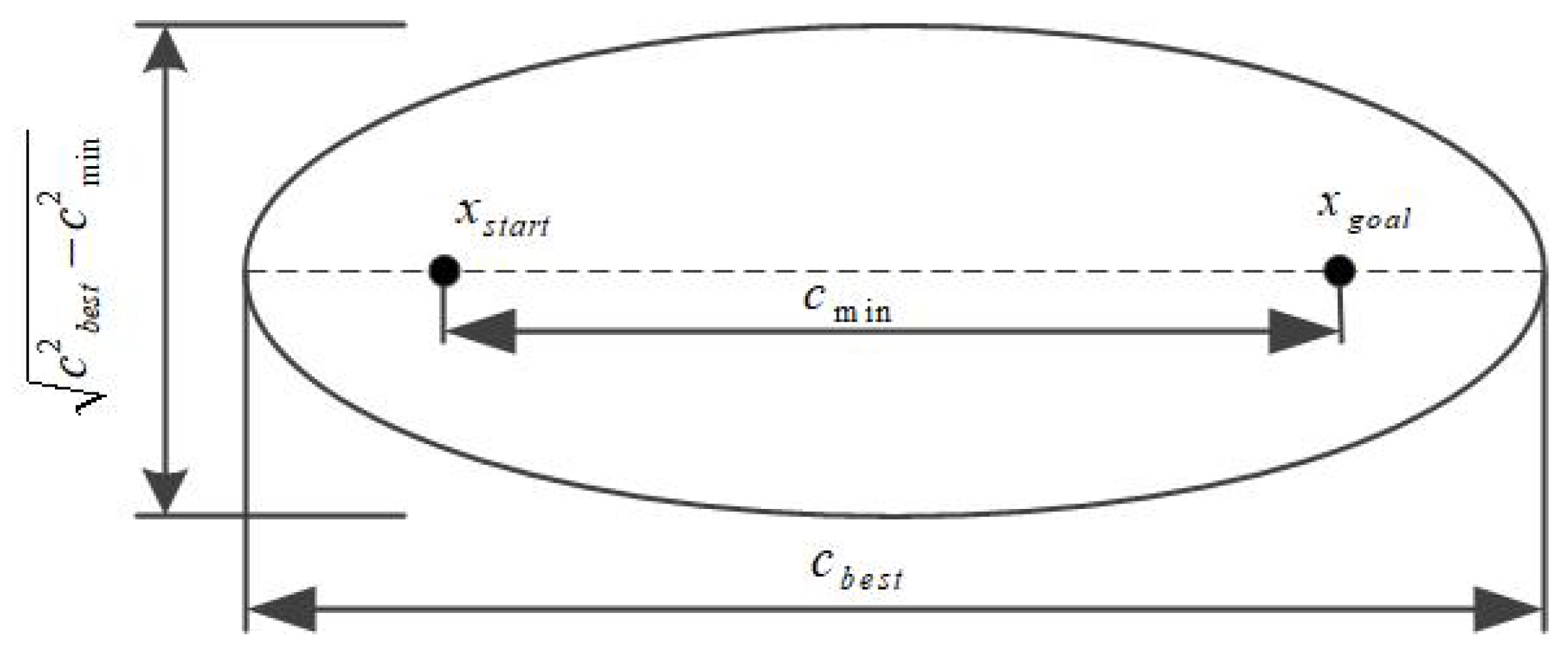
Informed RRT* utilizes an elliptical sampling strategy defined by $c_{\mathrm{best}}$ and $c_{\min }$, as illustrated in Figure 1. Here, $c_{\min }$ represents the Euclidean distance between $x_{\mathrm{start}}$ and $x_{\mathrm{goal}}$, while $c_{\mathrm{best}}$ corresponds to the cost of the first feasible path found by RRT*, serving as the major axis of the ellipse.

Once an initial path is obtained, Informed RRT* constructs the sampling ellipse by setting $c_{\mathrm{best}}$ as the major axis length $2a$ and $c_{\min }$ as the focal distance $2c$. The elliptical sampling space is then determined through Equations (1) and (2).

$$\begin{array}{c}\hfill {\displaystyle \frac{x^2}{a^2}}+{\displaystyle \frac{y^2}{b^2}}=1\end{array}$$

(1)

$$\begin{array}{c}\hfill a^2-c^2=b^2\end{array}$$

(2)

The Informed RRT* algorithm employs an elliptical sampling strategy to replace global uniform sampling, significantly improving computational efficiency. During each iteration, Informed RRT* performs sampling within the dynamically updated elliptical space, which contracts as shorter paths are discovered. This sampling mechanism accelerates the convergence rate, ultimately yielding shorter and more optimized paths [11]. The pseudo-code for the elliptical sampling function is presented in Algorithm 2.

Algorithm 2: InformedSample
	Input: $x_{start},x_{goal},C_{best}$
	Output: $x_{rand}$
1	if  $C_{best}<\infty$ then
2		$C_{min}\leftarrow {\Vert x_{goal}-x_{start}\Vert }_2$
3		$C_{center}={\displaystyle \frac{1}{2}}(x_{start}+x_{goal})$
4		$c\leftarrow RotationToWorldFrame(x_{start},x_{goal})$
5		$r_1\leftarrow {\displaystyle \frac{1}{2}}{C}_{best}$
6		for $i=2$ to n do
7			$r_i\leftarrow {\displaystyle \frac{1}{2}}\sqrt{C_{best}^2-C_{min}^2}$
8		end
9		$L\leftarrow diag\{r_1,\cdots ,r_n\}$
10		$X_{ball}\leftarrow SampleUnitBall$
11		$x_{rand}\leftarrow (cL{X}_{ball}+C_{center})\cap X$
12	end
13	else
14		$x_{rand}\leftarrow U\left(X\right)$
15	end
16	return $x_{rand}$

2.4. Informed RRT*

Informed RRT* consists of five core components: input initialization, main loop execution, node insertion and topology adjustment, path update, and optimized output generation. By incorporating heuristic constraints and optimizing the sampling space, Informed RRT* significantly enhances the performance of standard RRT*. The complete pseudo-code is provided in Algorithm 3.

Algorithm 3: Informed RRT*
	Input: $x_{start},x_{goal},X_{obs},Iter$
	Output: $T=(V,E)$
1	$V\leftarrow \left\{x_{start}\right\}$, $E\leftarrow ⌀$, $X_{soln}\leftarrow ⌀$
2	for $i=1$ to $Iter$ do
3		$C_{min}\leftarrow mi{n}_{X_{soln}\in X_{soln}}\left\{Cost\left(X_{soln}\right)\right\}$
4		$x_{rand}\leftarrow InformedSample(x_{start},x_{goal},C_{min})$
5		$x_{nearest}\leftarrow NearestNode(V,x_{rand})$
6		$x_{new}\leftarrow Steer(x_{rand},x_{nearest})$
7		if NoCollision($x_{nearest},x_{new},X_{obs}$) then
8			$X_{near}\leftarrow NearNode(V,x_{new})$
9			$x_{parent}\leftarrow ChooseParent(X_{near},x_{new},x_{nearest})$
10			$V\leftarrow V\cup \left\{x_{new}\right\}$
11			$E\leftarrow E\cup \left\{(x_{new},x_{parent})\right\}$
12			$G\leftarrow Rewire(G,X_{near},x_{new})$
13		end
14		if InGoalRegion($x_{new}$) then
15			$X_{soln}\leftarrow X_{soln}\cup \left\{x_{new}\right\}$
16		end
17	end
18	return  $T=(V,E)$

    The algorithmic workflow of Informed RRT* is as follows:

Step 1: Initialize input parameters, including start configuration $x_{\mathrm{start}}$, goal configuration $x_{\mathrm{goal}}$, obstacle space $X_{\mathrm{obs}}$, and maximum iteration count $Iter$. Initialize vertex set V, edge set E, tree structure $T=(V,E)$, and solution path set $X_{\mathrm{soln}}$.

Step 2: Compute the current optimal path cost $C_{\min }$ from $X_{\mathrm{soln}}$ and generate the heuristic sampling region. Sample a random configuration $x_{\mathrm{rand}}$ within this region and create a new node $x_{\mathrm{new}}$ by extending from $x_{\mathrm{nearest}}$ with a predefined step size.

Step 3: If the connection between $x_{\mathrm{nearest}}$ and $x_{\mathrm{new}}$ is collision-free, perform node insertion and topology optimization. The $ChooseParent$ procedure selects the optimal parent node for $x_{\mathrm{new}}$, while the $Rewire$ process attempts to connect $x_{\mathrm{new}}$ to nearby nodes in $X_{\mathrm{near}}$ to further reduce path cost.

Step 4: If $x_{\mathrm{new}}$ lies within the goal region, add it to $X_{\mathrm{soln}}$, and update $C_{\min }$ accordingly.

Step 5: Output the final tree structure $T=(V,E)$ and the optimal path from $X_{\mathrm{soln}}$.   

3. Improved Informed RRT* Algorithm

Informed RRT* improves sampling efficiency by incorporating heuristic guidance to avoid low-priority regions. During each iteration, the algorithm restricts sampling to a dynamically updated ellipsoidal search space, which is determined by the current optimal path length and heuristic information (e.g., the straight-line distance from start to goal). However, Informed RRT* requires an initial feasible path to establish this heuristic-guided search region. To accelerate convergence, two key improvements have been introduced: (1) a dynamic shrinkage threshold node selection mechanism and (2) an adaptive goal-biased strategy. These improvements significantly increase the efficiency of initial-path generation. The complete pseudo-code for the improved Informed RRT*, including the dynamic shrinkage threshold and adaptive goal-biased strategies, is provided in Algorithms 4–6.

Algorithm 4: Informed RRT*
	Input: $x_{start},x_{goal},X_{obs},Iter$
	Output: G=(V, E)
1	$V\leftarrow \left\{x_{start}\right\}$, $E\leftarrow ⌀$, $X_{soln}\leftarrow ⌀$
2	$r\leftarrow r_0$; $d\leftarrow d_0$;
3	for $i=1$ to $Iter$ do
4		$C_{min}\leftarrow mi{n}_{X_{soln}\in X_{soln}}\left\{Cost\left(X_{soln}\right)\right\}$
5		$x_{rand}\leftarrow InformedSample(x_{start},x_{goal},C_{min})$
6		$m\leftarrow Random(0,1)$; if $m>r$ then
7			$x_{target}\leftarrow x_{rand}$;
8		end
9		else
10			$x_{target}\leftarrow x_{goal}$;
11		end
12		$x_{nearest}\leftarrow NearestNode(V,x_{target})$
13		$x_{new}\leftarrow Steer(x_{target},x_{nearest})$
14		if NoCollision($x_{nearest},x_{new},X_{obs}$) then
15			$X_{near}\leftarrow NearNode(V,x_{new})$
16			$x_{parent}\leftarrow ChooseParent(X_{near},x_{new},x_{nearest})$
17			$V\leftarrow V\cup \left\{x_{new}\right\}$
18			$E\leftarrow E\cup \left\{(x_{new},x_{parent})\right\}$
19			$G\leftarrow Rewire(G,X_{near},x_{new})$
20			$hasNodeInRadius\leftarrow False$; foreach $x\in V$ do
21				if $Distance(x,x_{new})<d$ then
22					$hasNodeInRadius\leftarrow True$; break;
23				end
24			end
25			if $hasNodeInRadius$ then
26				$V\leftarrow V\setminus \left\{x_{new}\right\}$;
27			end
28			$r\leftarrow AdaptiveRate\left(r_0\right)$; $d\leftarrow AdaptiveD\left(d_0\right)$;
29		end
30		if InGoalRegion($x_{new}$) then
31			$X_{soln}\leftarrow X_{soln}\cup \left\{x_{new}\right\}$
32		end
33	end
34	return $G=(V,E)$

Algorithm 5: AdaptiveD function
	Input: alpha, i, iter, nobs, Sobs, S
	Output: d
1	$N_1\leftarrow nobs$
2	$N_2\leftarrow Sobs/S$
3	$d\leftarrow \alpha \ast (1-i/iter)/(N_1\ast e^{N_2})$
4	return d

Algorithm 6: AdaptiveRate function
	Input: $r_0$
	Output: r
1	$n_{pass},n_{total},S_{pass},S_{total}\leftarrow$ getObstacleInfo()
2	$C_{nobs}\leftarrow n_{pass}/n_{total}$
3	$C_{sobs}\leftarrow S_{pass}/S_{total}$
4	if $r\ne r_0$  then
5		$r\leftarrow r_0/e^{(C_{nobs}+C_{sobs})}$
6	end
7	else
8		$r\leftarrow 1$
9	end
10	if isInitialPathGenerated() then
11		$r\leftarrow 0$
12	end
13	return r

3.1. Dynamic Shrinkage Threshold Node Selection Mechanism

The node selection mechanism improves exploration efficiency by reducing redundancy. In this mechanism, once a $x_{\mathrm{new}}$ is explored, the distance between $x_{\mathrm{new}}$ and its neighboring nodes is calculated. If the distance exceeds the node selection threshold d, then $x_{\mathrm{new}}$ is added to the random tree; otherwise, the node is pruned to avoid unnecessary expansion [32]. Figure 2 illustrates the node selection mechanism, with black circles denoting the node selection threshold.

In this mechanism, the node selection threshold is a critical parameter. In simple environments with low complexity, path planning is relatively straightforward. Setting a small threshold has minimal impact on improving algorithmic efficiency. Conversely, a small threshold may lead to excessive sampling and redundant computations, thereby reducing efficiency. Therefore, in simple environments, selecting a larger threshold can effectively reduce sampling points and computational complexity while improving algorithmic efficiency. However, in obstacle-dense environments, a larger threshold may restrict the search space, degrade path quality, or even prevent the complete exploration of feasible paths. Hence, in high-complexity environments, a smaller threshold should be chosen to increase sampling density and optimize path planning. Additionally, heuristic guidance can restrict the sampling range, as the path is optimized, and the sampling range gradually narrows. In such cases, the node selection mechanism might lead to insufficient exploration within the sampling range, potentially omitting optimal paths and affecting the quality of the final planning results.

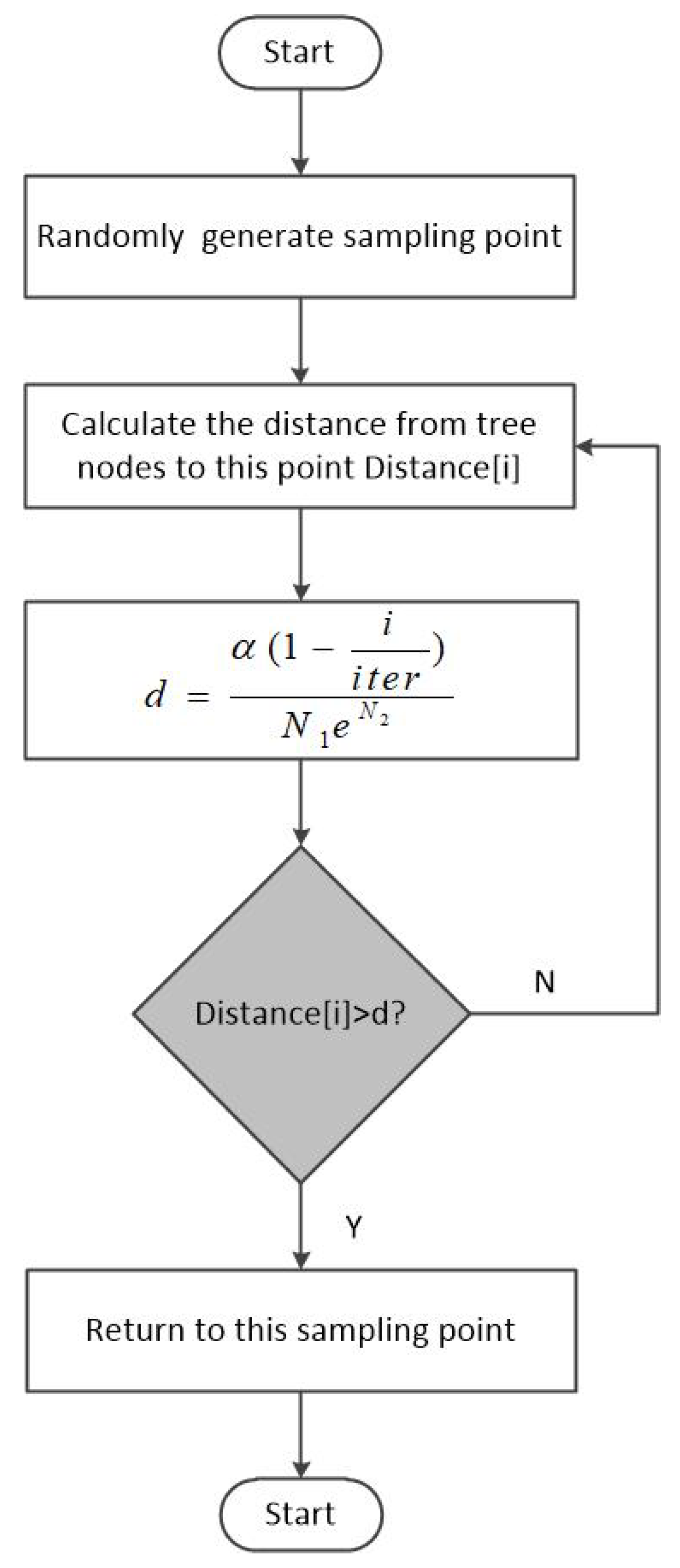
To address these limitations, this paper proposes a dynamic threshold shrinking node selection mechanism, as illustrated in Figure 3. The mechanism adaptively adjusts the node selection threshold based on environmental complexity and optimization progress, ensuring efficient exploration while maintaining path quality.

The improved method introduces a dynamic adjustment strategy based on the traditional node selection mechanism. By incorporating obstacle information from the map, the initial selection threshold is determined. Additionally, the method implements a threshold shrinking strategy, where the node selection threshold gradually decreases during the iteration process. This design effectively prevents the omission of potential optimal paths in later iterations caused by a reduced sampling range and excessively large selection thresholds. Consequently, it significantly improves the algorithm’s path optimization capability and global exploration performance.

The method for calculating the node selection threshold d is shown in Equations (3)–(5):

$$\begin{array}{c}\hfill d={\displaystyle \frac{\alpha (1-\frac{i}{iter})}{N_1{e}^{N_2}}}\end{array}$$

(3)

$$\begin{array}{c}\hfill N_1=n_{obs}\end{array}$$

(4)

$$\begin{array}{c}\hfill N_2={\displaystyle \frac{S_{obs}}{S}}\end{array}$$

(5)

where $\alpha$ is the limit parameter of the threshold, ensuring the node selection threshold remains within a reasonable range; S denotes the total area of the environment; i represents the current iteration count; $iter$ is the total number of iterations; $N_1$ indicates the number of obstacles; and $N_2$ is the ratio of the obstacle area to the total environmental area.

3.2. Adaptive Goal-Biased Strategy

The goal-biased strategy significantly improves the efficiency of reaching the goal point and reduces the time required to find feasible paths. The core idea is to increase the probability of selecting the goal point as a sampling point during random sampling, thereby accelerating tree expansion toward the target region [33]. This strategy ensures that the improved algorithm maintains strong target orientation. By incorporating the goal-biased strategy, the algorithm reduces the number of iterations needed to find the target path. Consequently, it enables the rapid exploration of the goal region, particularly in scenarios where the distance between the start and goal points is long.

The selection of goal-biased probability significantly impacts algorithm performance. In complex environments with numerous obstacles, the random tree may frequently encounter blockages when attempting to expand toward the goal point. If the goal-biased probability is set too high, finding feasible paths to bypass obstacles becomes challenging. Therefore, in complex environments, it is advisable to reduce the goal-biased probability and increase the frequency of random expansion, enabling the random tree to explore the environment more comprehensively and generate feasible paths. Conversely, in environments with fewer obstacles where path planning is simpler, increasing the goal-biased probability accelerates expansion toward the goal point, thereby improving algorithm efficiency. In practical applications, different environments require different goal-biased probabilities. Thus, this parameter typically needs to be experimentally adjusted and optimized to achieve a balance between exploration efficiency and comprehensiveness.

To address this issue, an adaptive goal-biased strategy is proposed, capable of calculating the goal-biased probability in real time based on the obstacle information along the line connecting the passing node $x_{nearest}$ and the goal point. This approach enables the algorithm to adjust its search strategy in real time based on real-time obstacle information, avoiding excessive bias towards the target point that may cause ineffective expansion in complex environments while enabling rapid expansion towards the target point in simpler environments. With this strategy, the algorithm maintains good versatility and adaptability in different complex environments. Figure 4 shows a detailed schematic of the adaptive goal-biased strategy, with the green circle representing obstacles.

This strategy determines the goal-biased probability r based on calculating the obstacle information along the line between $x_{neares{t}_1}$ and $x_{goal}$ by using the formula during the expansion of node $x_{neares{t}_1}$. When extended to $x_{neares{t}_2}$, due to the absence of obstacles along the connecting line, the bias probability r is set to 1, and the random tree grows directly towards the target point. This strategy enables the algorithm to quickly bypass obstacles and find feasible paths in complex environments while rapidly expanding towards the target point in simpler environments, enhancing the generation speed of initial paths and improving the algorithm’s efficiency.

The formula for computing the target bias probability r is provided in Equations (6)–(8).

$$\begin{array}{c}\hfill r={\displaystyle \frac{r_0}{e^{(C_{nobs}+C_{sobs})}}}\end{array}$$

(6)

$$\begin{array}{c}\hfill C_{nobs}={\displaystyle \frac{n_{pass}}{n_{total}}}\end{array}$$

(7)

$$\begin{array}{c}\hfill C_{sobs}={\displaystyle \frac{S_{pass}}{S_{total}}}\end{array}$$

(8)

where $r_0$ represents the maximum bias probability, $c_{nobs}$ denotes the ratio of the number of obstacles intersected by the line to the total number of obstacles, and $c_{sobs}$ indicates the ratio of the area of obstacles intersected by the line to the total obstacle area. Additionally, $n_{pass}$ is the number of obstacles the line crosses, $n_{total}$ is the total number of obstacles, $s_{pass}$ represents the area of obstacles intersected by the line, and $s_{total}$ denotes the total area of the map.

Adaptive Probability Adjustment: When $r=r_0$, both $c_{nobs}$ and $c_{sobs}$ are equal to 0, indicating that no obstacles exist along the connection. Consequently, r is set to 1, allowing the tree to expand directly towards the goal point, thereby accelerating the generation of the initial path. Once the initial path is obtained, elliptical heuristic information becomes available to guide the search, and r is subsequently set to 0 to prevent the omission of potential feasible paths.

4. Simulation Results and Analysis

In this section, comparative experiments in a two-dimensional space are conducted to verify the performance of the improved algorithm against the original algorithm. The experiments were performed on a computer equipped with an Intel^® Core^TM i7-10700 CPU @ 2.90 GHz (Intel Corporation, Santa Clara, CA, USA). The algorithm was implemented in Python 3.12, and the operating system used was Windows 10.

4.1. Algorithm Visualization Settings

Figure 5 depicts experimental environment 1, a simple environment characterized by sparse obstacles with dimensions of 20 m × 17 m. Figure 6 depicts experimental environment 2, a complex environment characterized by dense obstacles with dimensions of 20 m × 17 m. Figure 7 depicts experimental environment 3, featuring irregular obstacles and dimensions of 24 m × 17 m. The experiments are primarily conducted in these three environments. The start point for environments 1 and 2 is $(2,2)$, while the goal point is $(16,16)$. For environment 3, the start point is $(2,2)$, and the goal point is $(23,16)$. In the figures, the green areas represent obstacles, the purple points indicate nodes generated during the exploration process, the gray ellipse denotes the sampling range following the discovery of the first feasible path, and the blue and red lines represent the random tree and the feasible path, respectively.

4.2. Performance Comparison

An improved Informed RRT* is achieved by incorporating the dynamic shrinkage threshold node selection mechanism (hereafter abbreviated as A) and the adaptive goal-biased strategy (hereafter abbreviated as B). In this section, A and B are integrated with Informed RRT* to enhance its performance; further discussions are presented in the subsequent sections. The algorithms under analysis include (i) RRT with fixed bias parameters for the goal-biased strategy (hereafter abbreviated as RRT), (ii) RRT* with fixed bias parameters for the goal-biased strategy (hereafter abbreviated as RRT*), (iii) Informed RRT* with fixed bias parameters for the goal-biased strategy (hereafter abbreviated as IRRT*), (iv) Informed RRT* integrated with A (hereafter abbreviated as A-IRRT*), (v) Informed RRT* integrated with B (hereafter abbreviated as B-IRRT*), and (vi) Informed RRT* integrated with both A and B (hereafter abbreviated as AB-IRRT*). Ten experiments are conducted in this section; the experimental data are summarized and compared, demonstrating the superiority of the proposed method.

4.3. Key Parameters of the Algorithm

Step size: The step size defines the distance that the algorithm advances in each iteration. A smaller step size enhances the algorithm’s accuracy, albeit at the expense of slower convergence. Conversely, a larger step size accelerates convergence, though it may result in a less precise exploration of the solution space. Therefore, selecting an appropriate step size involves a trade-off between accuracy and computational efficiency, with the optimal value typically determined through experimental tuning.

$\alpha$: The threshold limit parameter, $\alpha$, is a key factor in the dynamic shrinkage threshold node selection mechanism (Method A). Its purpose is to constrain the node selection threshold, d, within a reasonable range. Method A dynamically adjusts the node selection threshold, d, based on the environmental complexity prior to the commencement of iterations. However, it is imperative to ensure that d remains within acceptable bounds. If d is too large, it will be difficult to find better paths. On the other hand, if d is too small, the improvement effects will be poor.

$r_0$: The maximum bias probability, $r_0$, functions similarly to the previously mentioned threshold limit parameter, serving as a constraint for the bias probability, r, within the adaptive goal-biased strategy (Method B). This constraint ensures that the bias probability does not become excessively high, which could lead the algorithm to converge to local optima or impede its ability to navigate around obstacles in environments with high obstacle density.

r: The proposed strategy aims to enhance the speed of initial-solution generation, thereby accentuating the heuristic guidance inherent in the Informed RRT* algorithm and expediting the path optimization process. Consequently, in the experiments, the goal-bias probability, r, is incorporated into the classic algorithms—RRT, RRT*, and Informed RRT*—to enhance their initial-solution generation speed, and comparative experiments are subsequently conducted with the improved algorithm. The impact of this parameter on algorithm performance has been discussed in detail in the introduction to $r_0$.

The selection of these parameters is typically contingent upon specific application requirements and environmental complexity. During the algorithm tuning phase, these parameters may be adjusted experimentally. The step size and r may be initialized at small values and subsequently adjusted based on convergence speed and accuracy requirements, while the parameters $\alpha$ and $r_0$ can be determined in accordance with environmental complexity to effectively govern node selection and the goal-biased strategy, thereby achieving an optimal balance between convergence speed and path quality.

4.4. Sparse Map

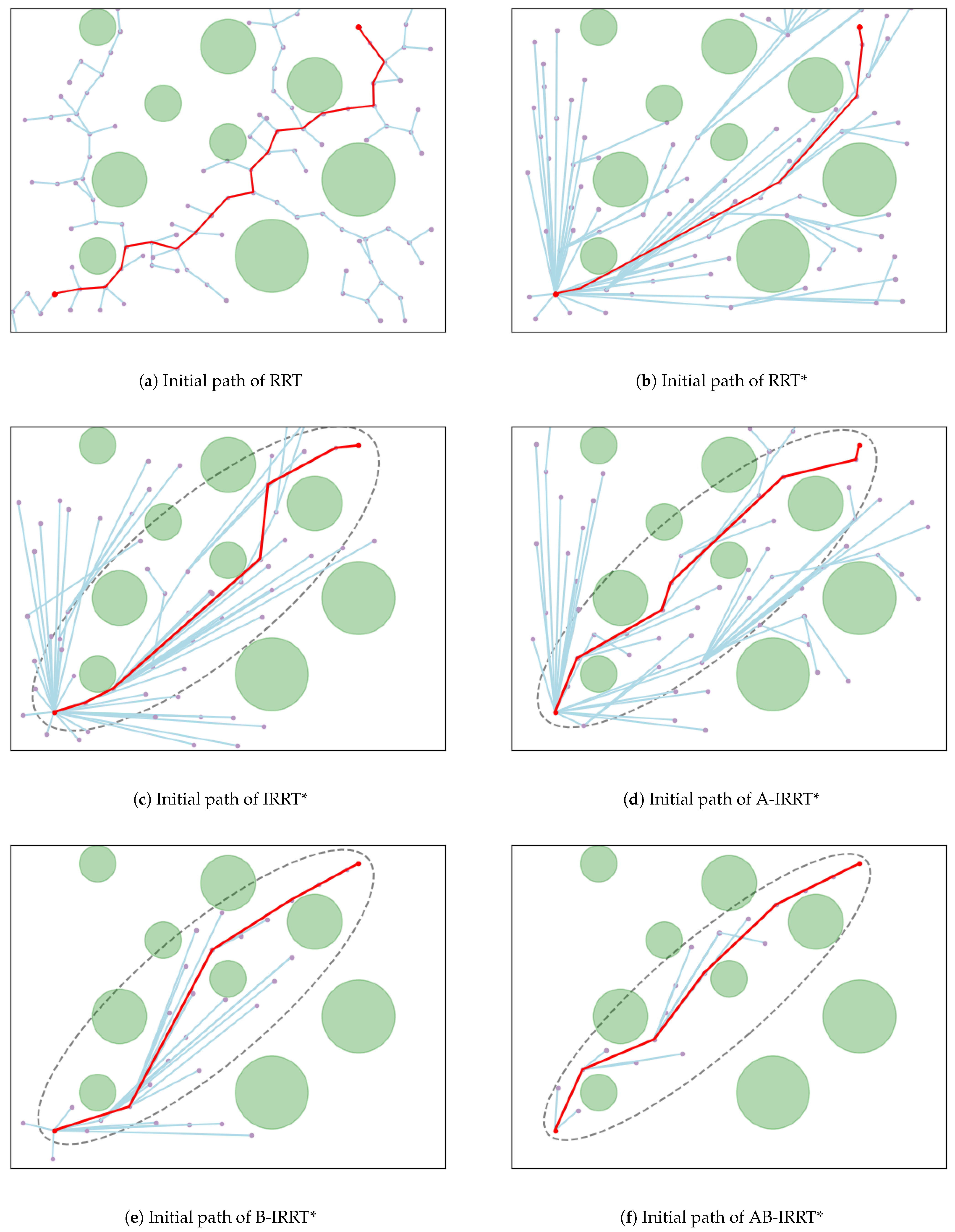
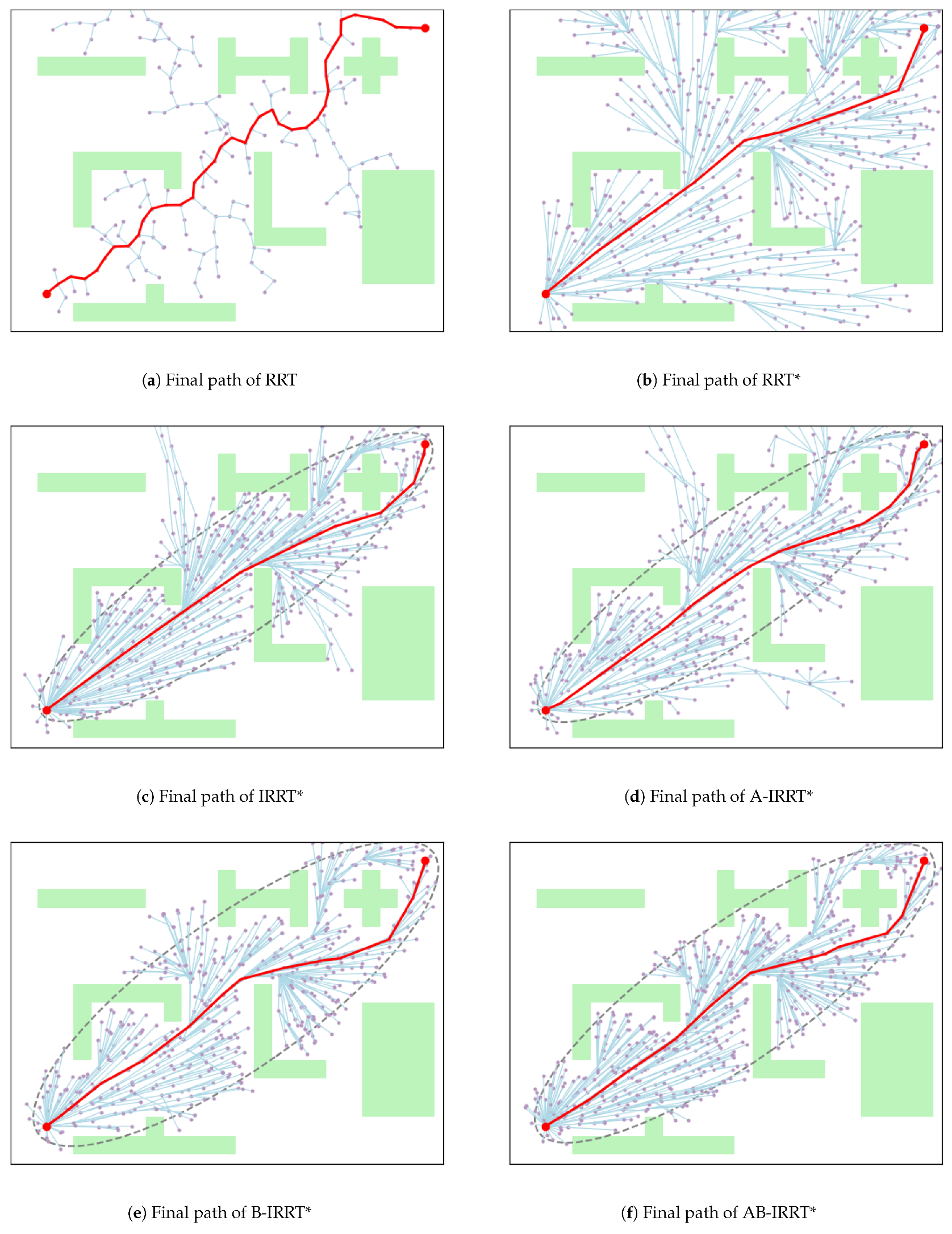
The parameter settings for the algorithms in the sparse map are as follows: step size = 1.5, threshold limit parameter $\alpha =5$, total number of iterations $iter=500$, maximum bias probability $r_0=0.14$, and fixed threshold goal-bias probability $r=0.1$. The initial and final paths produced by the six algorithms in the sparse map are presented in Figure 8 and Figure 9, respectively. Figure 10 and

Table 1. Simulation data for sparse maps.

Algorithm	Average Path Length (m)	Average Running Time (s)
RRT	26.8268	7.0541
RRT*	20.7739	6.9025
IRRT*	20.8389	6.9187
A-IRRT*	20.7365	7.7984
B-IRRT*	20.3430	2.8132
AB-IRRT*	20.2941	2.0541

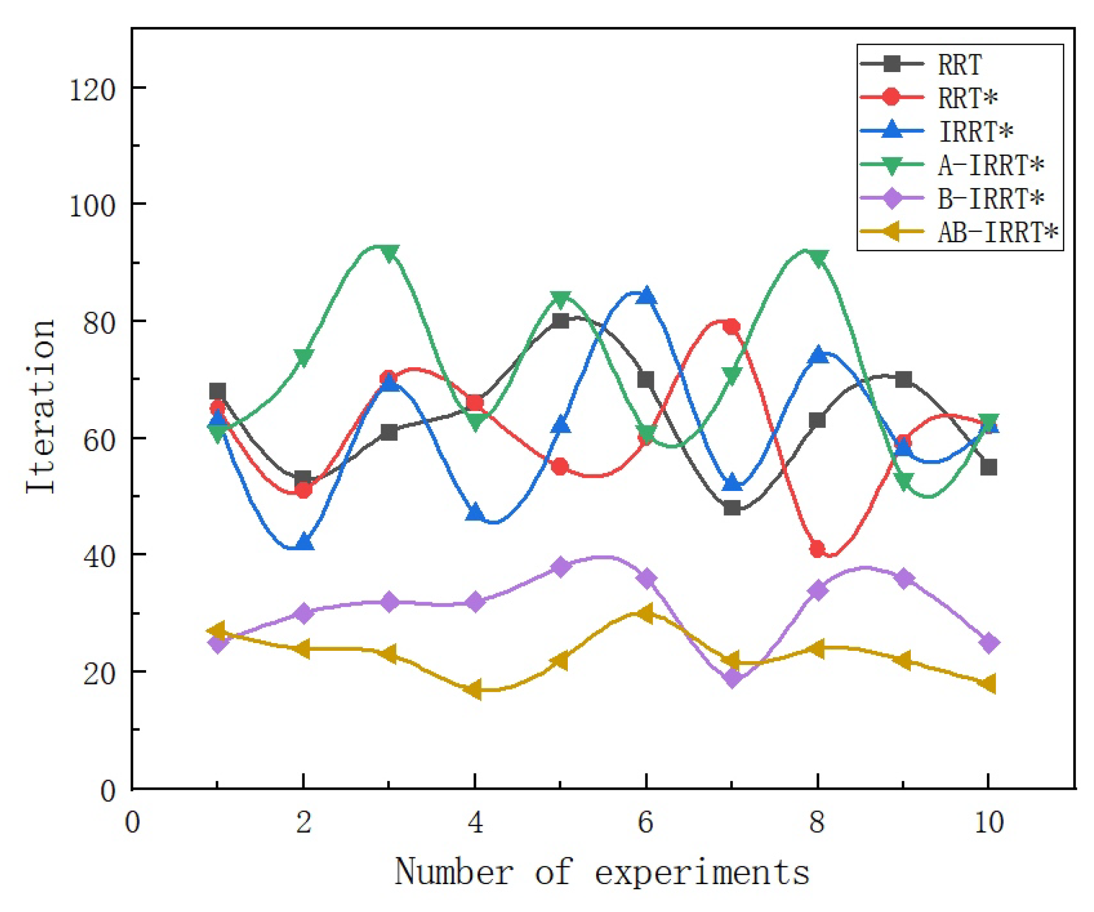
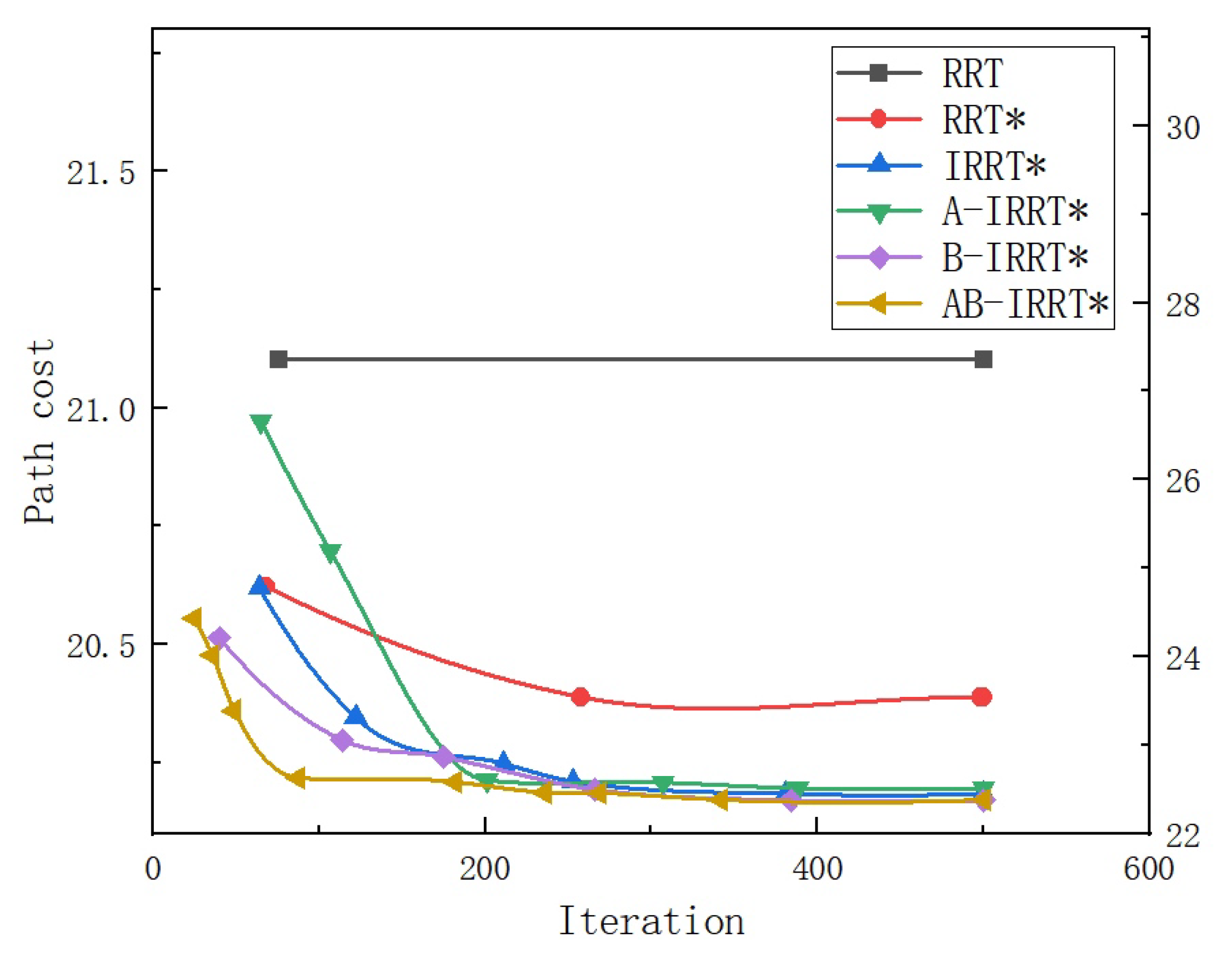
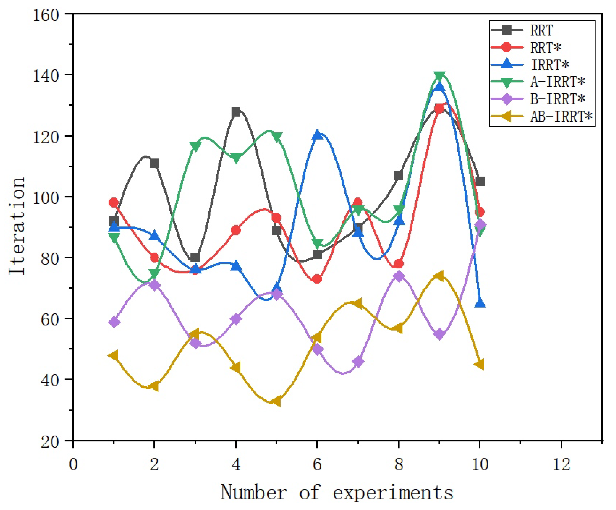
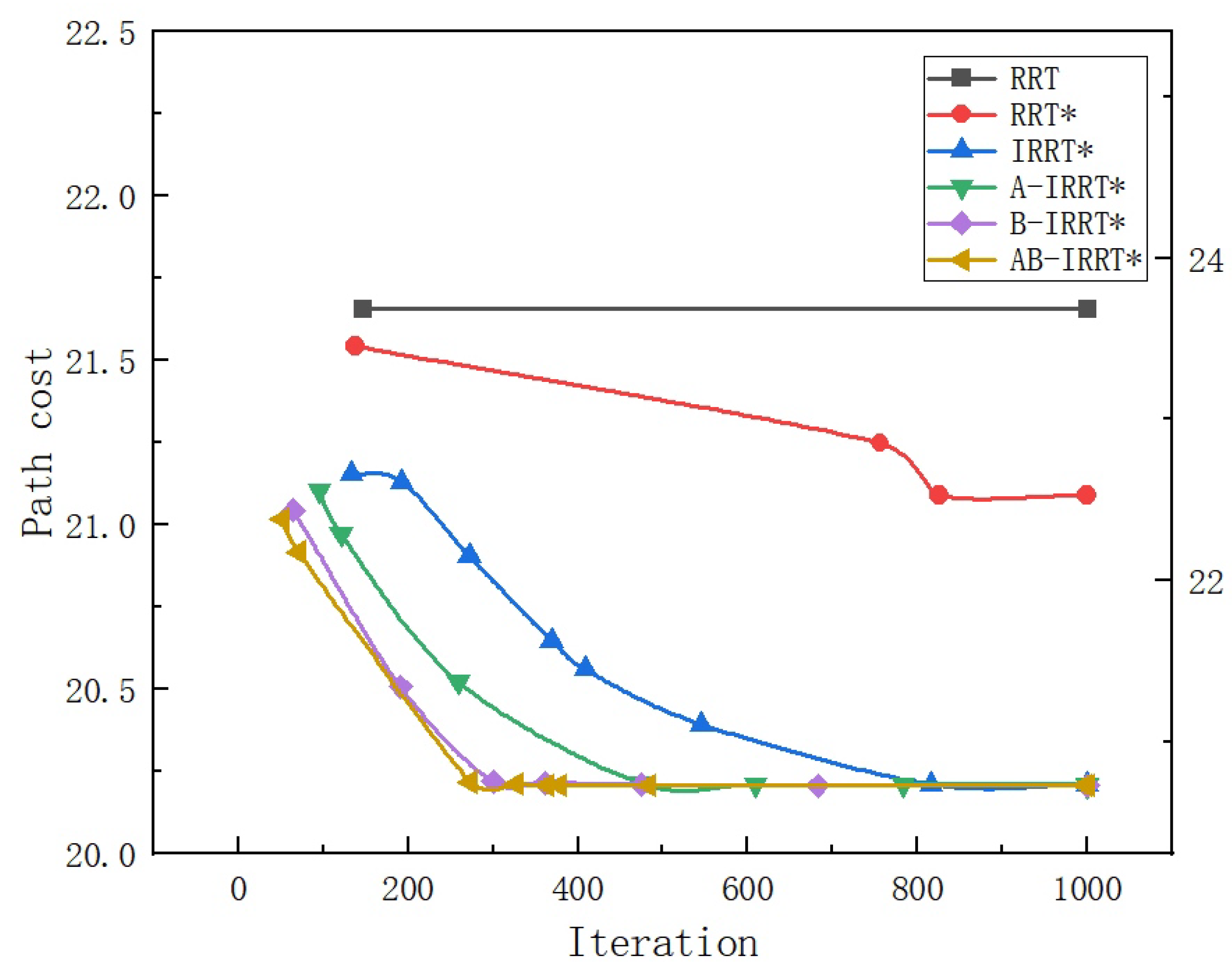
present the performance metrics of the six algorithms in the simple map. In Figure 10, black diamonds denote outliers, black squares indicate mean values, and the black line within the box denotes the median. Figure 11 displays the number of iterations required to generate initial paths by the six algorithms over ten experiments, while Figure 12 illustrates the relationship between path length and the number of iterations throughout the entire iterative process. Note: Due to the excessively long initial path produced by the RRT algorithm, for ease of observation in Figure 12, the path length of the RRT algorithm is scaled according to the axis on the right side.

From Figure 8, the characteristics of initial-path generation for various algorithms in environment 1 are as follows: The RRT algorithm, due to its lack of optimization, produces a zigzag path of greater length; RRT* and its variants significantly improve path quality; A-IRRT* and AB-IRRT* expand the exploration range by filtering out nearby nodes, thereby enhancing generation efficiency; and B-IRRT* and AB-IRRT* employ adaptive goal-bias probability adjustments to rapidly expand towards the goal under sparse-obstacle conditions, markedly accelerating initial-solution generation. From Figure 9, the convergence characteristics of the six algorithms are observed as follows: The path produced by the RRT algorithm remains unchanged, retaining its initial form due to the absence of optimization; RRT* exhibits limited path optimization after 500 iterations owing to the lack of elliptical sampling constraints; and A-IRRT*, B-IRRT*, and AB-IRRT* accelerate initial-solution generation through improved strategies, resulting in shorter path lengths after iterations and demonstrating superior convergence efficiency relative to the other algorithms. According to the data in Table 1, the RRT algorithm generates significantly longer paths than the other algorithms because of its lack of path optimization. RRT, RRT*, and IRRT* display similar performance in initial-solution generation, with minimal differences in their strategies. Compared with IRRT*, A-IRRT*, B-IRRT*, and AB-IRRT* reduce the initial solution path length by 0.49%, 2.38%, and 2.61%, respectively. In terms of runtime, B-IRRT* and AB-IRRT* decrease the time by 59.34% and 70.31%, whereas A-IRRT* results in a 12.71% increase. From the box plot in Figure 10 and the fluctuation curve of initial-solution iterations in Figure 11, it is evident that RRT, RRT*, and IRRT* exhibit little difference in the speed and stability of initial-solution generation; B-IRRT* and AB-IRRT* significantly enhance both speed and stability; and A-IRRT* is slightly inferior to IRRT* in these respects. Figure 12 illustrates the trends in path length optimization during the iterations of the six algorithms. Owing to the absence of path optimization steps, the RRT algorithm maintains an unchanged path length throughout iterations. In contrast, RRT* demonstrates less effective optimization compared with the IRRT* series algorithms due to the lack of elliptical sampling constraints. B-IRRT* and AB-IRRT*, benefiting from faster initial-solution generation, commence path optimization within the elliptical region earlier, thereby substantially improving optimization efficiency and achieving the asymptotically optimal path more rapidly. In comparison, the path optimization speed of A-IRRT* is similar to that of IRRT* and does not exhibit any significant advantages.

The results indicate that in environment 1, B-IRRT* and AB-IRRT* outperform IRRT* in terms of initial-solution generation speed, path quality, and stability, whereas A-IRRT* exhibits comparatively inferior performance. However, further analysis reveals that this outcome stems from the relatively simple and regular geometry of obstacles in environment 1, in which the optimization effect of the goal-biased strategy on initial-solution generation is particularly pronounced. Since A-IRRT* is the only algorithm among the six that does not incorporate the goal-biased strategy, its performance in this environment is inferior to that of IRRT*. It is important to emphasize that this observation does not imply that Strategy A is ineffective. As demonstrated by the superior performance of AB-IRRT* compared with B-IRRT*, Strategy A indeed contributes positively to the algorithm’s improvement. However, in this specific environment, the pronounced effect of the goal-biased strategy tends to mask the advantages of Strategy A.

4.5. Dense Map

The parameter settings for the algorithms in the dense map are as follows: step size = 1.2, $\alpha =5$, $iter=1000$, $r_0=0.14$, and $r=0.1$. The initial and final paths produced by the six algorithms in the dense map are shown in Figure 13 and Figure 14, respectively. Figure 15 compares the simulation results of the six algorithms in the dense map environment. The data in

Table 2. Simulation data for dense maps.

Algorithm	Average Path Length (m)	Average Running Time (s)
RRT	23.6051	12.4599
RRT*	21.2419	12.7657
IRRT*	21.2469	12.9332
A-IRRT*	21.3468	15.3558
B-IRRT*	20.8342	6.2727
AB-IRRT*	20.8080	5.0897

present the path length and runtime of the six experiments. Figure 16 displays the number of iterations required for generating initial paths by using the six methods over ten experiments, while Figure 17 illustrates the relationship between path length and the number of iterations throughout the entire iterative process. Note: Due to the excessively long initial path produced by the RRT algorithm, for ease of observation in Figure 17, the path length of the RRT algorithm is scaled according to the axis on the right side.

From Figure 13, it can be observed that the initial-path generation performance of the algorithms in environment 2 varies markedly. The RRT algorithm produces winding and lengthy paths due to the absence of optimization, whereas RRT* and its variants enhance path quality. A-IRRT* and AB-IRRT* expand the search range by filtering out nearby nodes, thereby enhancing efficiency. B-IRRT* and AB-IRRT* leverage the goal-biased strategy to rapidly bypass obstacles and extend toward the goal, significantly accelerating initial-solution generation. Figure 14 shows that the RRT algorithm does not perform any path optimization, leaving its initial path unchanged. RRT*, which lacks the elliptical sampling constraint, exhibits inferior path optimization compared with the IRRT* series. A-IRRT*, B-IRRT*, and AB-IRRT*, by adopting improved strategies, accelerate initial-solution generation, resulting in significantly shorter path lengths after iterations and demonstrating higher convergence efficiency than the other algorithms. According to the data in Table 2, the RRT algorithm produces the longest paths. The strategies employed by RRT, RRT*, and IRRT* are similar, yielding comparable performance. Compared with IRRT*, B-IRRT* and AB-IRRT* reduce the initial solution path length by 1.94% and 2.07%, respectively, whereas A-IRRT* increases it by 0.47%. In terms of runtime, B-IRRT* and AB-IRRT* reduce the execution time by 51.50% and 60.65%, respectively, whereas A-IRRT* incurs an increase of 18.73%. From the box height in Figure 15 and the fluctuation of initial-solution iteration counts in Figure 16, it is evident that RRT, RRT*, and IRRT* exhibit minimal differences in the speed and stability of initial-solution generation. In contrast, B-IRRT* and AB-IRRT* significantly enhance both the speed and stability of initial-solution generation, while A-IRRT* performs slightly worse than IRRT*. Figure 17 illustrates that the path length of the RRT algorithm remains unchanged throughout iterations. RRT*, due to the absence of elliptical sampling, exhibits inferior optimization compared with the IRRT* series. Conversely, B-IRRT* and AB-IRRT*, benefiting from faster initial-solution generation, demonstrate higher optimization efficiency and achieve the asymptotically optimal path at an earlier stage. A-IRRT* achieves optimization at a rate slightly slower than that of B-IRRT* and AB-IRRT* yet remains faster than IRRT*.

These results indicate that in environment 2, B-IRRT* and AB-IRRT* outperform IRRT* in terms of initial-solution generation speed, path quality, and stability, whereas A-IRRT* exhibits relatively inferior performance. However, the superior performance of AB-IRRT* relative to B-IRRT* confirms the effectiveness of Strategy A, which is consistent with the findings in sparse maps. Moreover, during the iterative optimization phase following the generation of the initial solution, A-IRRT* achieves higher optimization efficiency than IRRT*. This demonstrates that although the goal-biased strategy with a fixed goal-bias probability facilitates faster initial-solution generation in environments characterized by regular obstacles, its fixed bias probability may impede effective navigation around obstacles in cluttered environments, thereby reducing path optimization efficiency. This also indirectly validates the advantages of the adaptive goal-biased strategy proposed in this study.

4.6. Irregular Map

In environments 1 and 2, which feature regularly shaped obstacles, the goal-biased strategy exhibits a more pronounced effect than Strategy A. To further validate the performance enhancements introduced by Strategy A, this section evaluates the proposed algorithms in environments characterized by irregular obstacles, including H-shaped, U-shaped, and L-shaped configurations [34].

The parameter settings for the algorithms in the irregular map are as follows: step size = 0.8, $\alpha =5$, $iter=1000$, $r_0=0.14$, and $r=0.1$. The initial and final paths generated by the six algorithms in the irregular map are depicted in Figure 18 and Figure 19, respectively. Figure 20 presents a comparison of the simulation results of the six algorithms in an irregular map environment. The data in

Table 3. Simulation data for irregular maps.

Algorithm	Average Path Length (m)	Average Running Time (s)
RRT	30.3328	15.6027
RRT*	27.2920	13.7907
IRRT*	27.2944	14.4281
A-IRRT*	27.2185	5.8490
B-IRRT*	27.2826	7.5341
AB-IRRT*	27.2489	4.9244

present the path length and runtime of the six experiments. Figure 21 illustrates the number of iterations required to generate initial paths by using the six methods across ten experiments, while Figure 22 depicts the relationship between path length and iteration count throughout the entire process. Note: Due to the excessively long initial path produced by the RRT algorithm, for ease of observation in Figure 22, the path length of the RRT algorithm is scaled according to the axis on the right side.

From Figure 18, the characteristics of initial-path generation for each algorithm in environment 3 can be summarized as follows: The RRT algorithm, due to the absence of optimization steps, generates paths that are not only tortuous but also relatively long. RRT* and its variants notably enhance path quality. A-IRRT* and AB-IRRT* expand the exploration space by filtering out nearby nodes, thereby improving efficiency. B-IRRT* and AB-IRRT* effectively bypass obstacles and substantially reduce the time required to generate an initial solution by adaptively adjusting the target bias probability. From Figure 19, the convergence performance of the six algorithms is as follows: the RRT algorithm does not optimize the path, leaving it unchanged from the initial one. RRT*, lacking elliptical sampling constraints, exhibits limited path optimization after iterations. A-IRRT* and AB-IRRT* accelerate initial-solution generation through improved strategies, achieving better path lengths after iterations and indicating superior convergence efficiency. However, the optimization performance of B-IRRT* is slightly inferior. As shown in Table 3, the RRT algorithm, due to the lack of path optimization, produces paths that are significantly longer than those of other algorithms. RRT, RRT*, and IRRT* exhibit minimal differences in their initial-solution generation strategies, leading to comparable performance. Compared with IRRT*, the initial-path lengths of A-IRRT*, B-IRRT*, and AB-IRRT* are reduced by 0.28%, 0.04%, and 0.16%, respectively. In terms of runtime, the reductions for A-IRRT*, B-IRRT*, and AB-IRRT* relative to IRRT* are 47.80%, 59.46%, and 65.86%, respectively. By analyzing the box heights in Figure 20 and the oscillation curves of initial-solution iteration counts in Figure 21, it can be observed that RRT, RRT*, and IRRT* exhibit little difference in speed and stability during initial-solution generation, and their performance remains relatively poor. In contrast, A-IRRT*, B-IRRT*, and AB-IRRT* significantly enhance both speed and stability, with algorithms incorporating Strategy A demonstrating more pronounced advantages. From Figure 22, the optimization trends of path lengths during iterations for the six algorithms can be observed. The RRT algorithm, lacking path optimization steps, retains an unchanged path length throughout iterations. In comparison, RRT*, without elliptical sampling constraints, demonstrates significantly inferior path optimization performance compared with the IRRT* series under the same number of iterations. A-IRRT*, B-IRRT*, and AB-IRRT* exhibit significantly faster optimization speeds than IRRT*, but the final path length of B-IRRT* is slightly longer than that of A-IRRT* and AB-IRRT*.

These results indicate that in environment 3, A-IRRT* and AB-IRRT* outperform IRRT* in terms of initial-solution generation speed and stability, while B-IRRT* performs relatively worse than A-IRRT* and AB-IRRT*. Further analysis reveals that this discrepancy arises from the irregularity of obstacles in environment 3. Strategy B dynamically adjusts the bias probability to facilitate the rapid extension of the random tree toward the target point. However, the presence of cross-shaped obstacles near the target, particularly their concave regions, may lead this mechanism to overlook certain feasible paths, as illustrated in Figure 19. By integrating Strategies A and B, this issue is effectively mitigated, further demonstrating that Strategy A provides greater advantages in environments with irregular obstacles compared with the goal-biased strategy. This conclusion is consistent with the analyses of environments 1 and 2.

4.7. Calculation of Resource Consumption

In the practical application of path-planning algorithms, memory usage and computational resource consumption are critical metrics for evaluating algorithm performance, especially in resource-constrained embedded or real-time systems. To comprehensively assess the practical value of the proposed algorithm, a detailed comparative analysis of CPU utilization and memory usage during its execution is provided in this section.

During the execution of the algorithm, the CPU is primarily responsible for computation and logical processing, such as random point generation, tree expansion and connection, collision detection, path planning, and the execution of search strategies. These tasks involve numerous mathematical operations, such as geometric distance calculations, random number generation, and the complex logic of collision detection. On the other hand, memory is mainly used to store data generated during the algorithm’s execution, such as the tree structure and node information, records of the search space, intermediate computation results, and the environment model. As the search progresses, memory usage gradually increases.

Table 4. Calculate resource data.

Algorithm	Average CPU Usage Rate (%)	Average Memory Usage Rate (%)
RRT	1.17	33.30
RRT*	1.31	33.46
IRRT*	1.45	33.37
A-IRRT*	2.20	33.38
B-IRRT*	1.66	33.50
AB-IRRT*	1.74	33.36

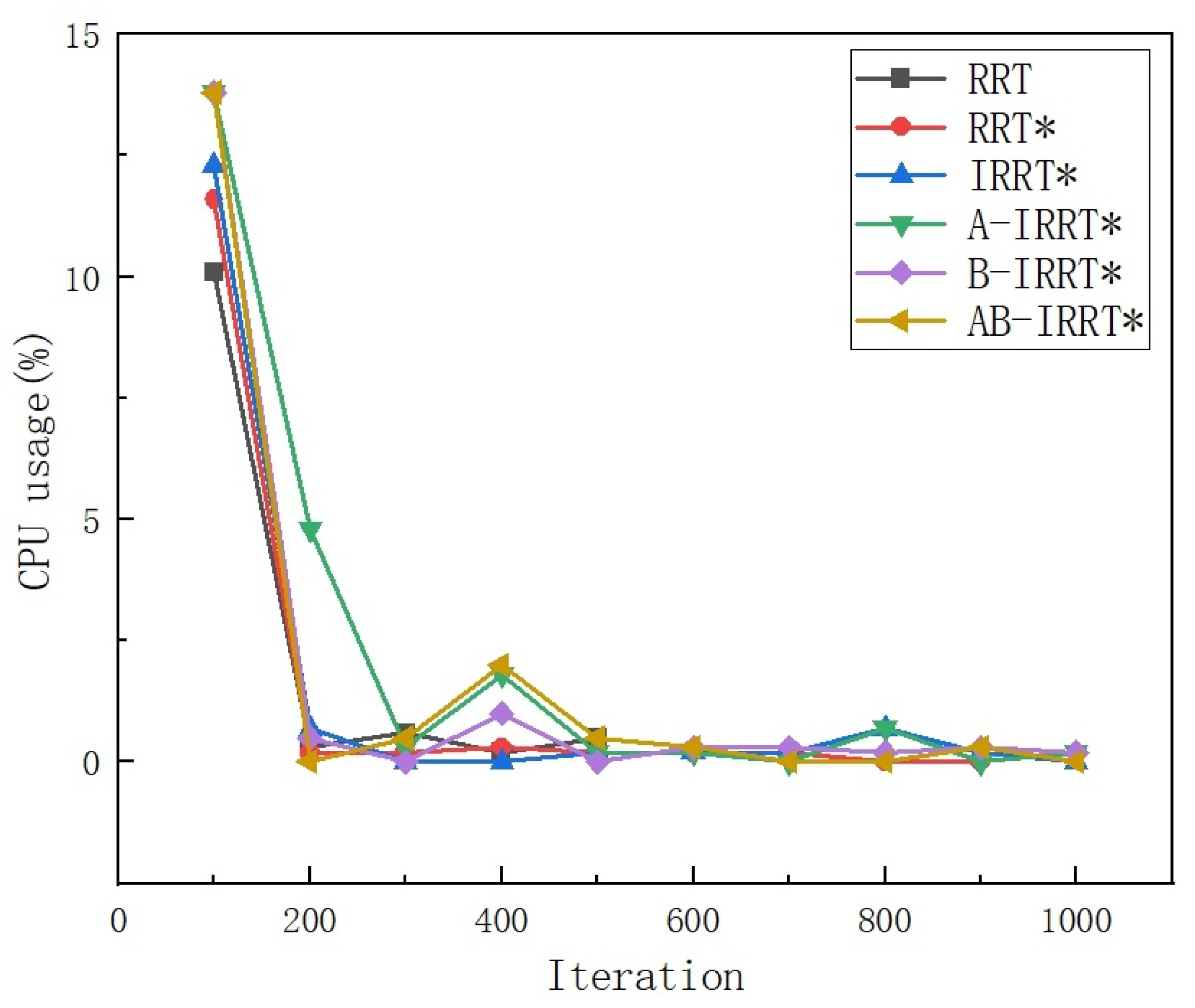
presents the average CPU and memory usage rates of the six algorithms during execution. Figure 23 illustrates the CPU usage variation curves of the six algorithms during runtime, while Table 4 shows the memory usage variation curves. Based on Table 4 and the CPU usage variation curve in Figure 23, it is evident that the RRT algorithm exhibits lower CPU usage than the other five algorithms due to the absence of a path optimization process. Additionally, the introduction of guided elliptical region sampling results in reduced memory usage for the four IRRT*-based algorithms compared with the other two. From Table 4 and the memory usage variation curve in Figure 24, it can be observed that the proposed methods have a minimal impact on memory usage, which is negligible. Since this study focuses on improving the IRRT* algorithm, the analysis centers on the four IRRT*-based algorithms. Specifically, in terms of CPU usage, A-IRRT* increased by 51.72%, B-IRRT* by 14.48%, and AB-IRRT* by 20.00%, all compared with IRRT*. It is evident that Method A leads to a more significant increase in CPU usage, while Method B exhibits only a slight improvement. In terms of memory usage, B-IRRT* increased by 0.39% compared with IRRT*, while fluctuations for A-IRRT* and AB-IRRT* remained within 0.03%.

In summary, Method A has a slightly larger impact on CPU usage, with a relatively smaller effect on memory usage. In contrast, Method B has a slightly larger effect on memory usage, with a smaller impact on CPU usage. When combined, these two methods have a minimal overall impact on both CPU and memory usage. Compared with the performance improvements brought by optimization, this slight increase in resource usage is acceptable.

4.8. Experimental Summary

Comparative experiments conducted on six algorithms in three different environments revealed that Strategies A and B each offer distinct advantages in generating initial solutions and enhancing algorithm efficiency. When obstacles are more regularly shaped (e.g., environments 1 and 2), Strategy B significantly enhances algorithm performance. In contrast, Strategy A performs better in environments with more complex obstacle shapes (e.g., environment 3). However, when Strategies A and B are combined, the algorithm exhibits strong robustness and adaptability across different environments. Subsequently, the computational resource usage of the two strategies, including CPU and memory usage, was analyzed. The results indicate that after combining Strategies A and B, the algorithm’s computational resource usage increases only slightly, and this minor increase is fully acceptable given the performance improvements achieved. Overall, the experimental results indicate that the combination of Strategies A and B significantly enhances the algorithm’s adaptability and robustness across different environments, achieving these improvements with minimal computational resource overhead. This demonstrates the substantial potential and advantages of the proposed method in enhancing path-planning efficiency and stability.

5. Robot Platform Simulation Experiment

In the previous section, the proposed improved algorithm was validated by using a point-mass model of a robot. However, when the algorithm is applied to an actual robotic platform, various practical challenges often arise. To further evaluate the performance of the improved AB-IRRT* algorithm on a real robotic platform, this section utilizes the Gazebo simulation environment within the ROS framework to create a scenario with unknown obstacles and dynamic pedestrians. This setup aims to simulate the complex situations that a robot may encounter during real-world navigation. Since this study focuses on global path planning and robot navigation also requires a local path-planning algorithm for dynamic obstacle avoidance, the proposed AB-IRRT* algorithm is combined with the classical DWA local path-planning algorithm for comprehensive testing. Since the robot needs to continuously adjust its path based on real-time environmental changes during navigation, studying the time and path length of global path planning in isolation would not be meaningful. Therefore, this section focuses on analyzing the path length and navigation time during the actual navigation process, in which the proposed AB-IRRT* algorithm is integrated with the local path-planning algorithm. The experiments are conducted in a simulated environment with dynamic and unknown obstacles to validate the navigation performance of the AB-IRRT* algorithm on a robotic platform, demonstrating its robustness in complex dynamic environments.

5.1. Environment Visualization Settings

The simulation environment for this experiment measures 24 m × 24 m. Figure 25 illustrates the simulation environment with unknown static obstacles, along with its corresponding map. As shown in the figure, the obstacles marked with red circles represent unknown obstacles, which were not included in the environment map during the mapping process. In this experimental scenario, the robot’s starting coordinates are set as $(0,0)$, with the goal coordinates set as $(4,9)$. Figure 26 depicts the simulation environment with dynamic pedestrians, along with its corresponding map. The dark-blue trajectory in the figure represents the movement paths of the pedestrians. In this scenario, the robot’s starting coordinates are set as $(0,0)$, with the goal coordinates set as $(5,-9)$. The shaded areas in the figure represent obstacle regions, while the white areas indicate the navigable space for the robot. The dark-green and light-green lines represent the generated random tree and the feasible path planned by the algorithm, respectively.The red line represents the path traveled by the robot during navigation.

5.2. Comparative Experiment in an Environment with Unknown Static Obstacles

This section integrates the proposed AB-IRRT* algorithm with the DWA algorithm and conducts five navigation experiments in an environment containing unknown obstacles. Figure 27 illustrates the global paths planned by the IRRT* and AB-IRRT* algorithms at the beginning of the navigation process. Figure 28 illustrates the actual paths traveled by the two algorithms during the navigation process.

Table 5. Experimental results of actual navigation path length in an environment with unknown static obstacles.

Path	IRRT*		AB-IRRT*
No.	Path Length (m)	Average Length (m)	Path Length (m)	Average Length (m)
1	12.8652	12.8725	12.7728	12.6982
2	12.9236		12.7124
3	12.8230		12.6216
4	12.7851		12.6319
5	12.9658		12.7253

presents the path lengths traveled by the robot, along with their averages, in the five experiments for both algorithms.

Table 6. Experimental results of actual navigation time in an environment with unknown static obstacles.

Path	IRRT*		AB-IRRT*
No.	Running Time (s)	Average Time (s)	Running Time (s)	Average Time (s)
1	59.4328	59.0467	56.1327	56.8202
2	57.5814		58.0581
3	60.0268		55.8653
4	59.2458		57.1497
5	58.9463		56.8952

presents the navigation times and their averages for both algorithms across the five experiments.

As shown in Figure 28, the AB-IRRT* algorithm generates a smoother path during robot navigation compared with the IRRT* algorithm. According to the data in Table 5, the average path length traveled by the AB-IRRT* algorithm during navigation is reduced by 1.35% compared with that of the IRRT* algorithm. The data in Table 6 show that the average navigation time for the AB-IRRT* algorithm is reduced by 3.78% compared with that of the IRRT* algorithm. These results indicate that the proposed AB-IRRT* algorithm, when applied to the robotic platform, optimizes both the path length and navigation time while also improving the smoothness of the navigation path.

5.3. Comparative Experiment in an Environment with Dynamic Pedestrians

In this section, the proposed AB-IRRT* algorithm is combined with the DWA algorithm, and five navigation experiments are conducted in an environment with dynamic pedestrians. Figure 29 illustrates the global paths planned by the IRRT* and AB-IRRT* algorithms at the beginning of the navigation process. Figure 30 illustrates the actual paths traveled by the robot during navigation with both algorithms.

Table 7. Experimental results of actual navigation path length in an environment with dynamic pedestrians.

Path	IRRT*		AB-IRRT*
No.	Path Length (m)	Average Length (m)	Path Length (m)	Average Length (m)
1	11.8749	12.8491	11.6371	11.6567
2	12.5417		10.9853
3	13.9509		12.2841
4	12.7940		11.0674
5	13.0842		12.3097

summarizes the path lengths traveled by the robot, along with their averages, in the five experiments for both algorithms.

Table 8. Experimental results of actual navigation time in an environment with dynamic pedestrians.

Path	IRRT*		AB-IRRT*
No.	Running Time (s)	Average Time (s)	Running Time (s)	Average Time (s)
1	50.9352	52.5732	49.4508	49.5190
2	53.2780		48.8639
3	52.9643		50.0376
4	50.8279		47.9935
5	54.8607		51.2490

provides the navigation times and their averages for both algorithms across the five experiments.

As shown in Figure 29, the AB-IRRT* algorithm generates a smoother path during navigation compared with the IRRT* algorithm. According to the data in Table 7, the average path length traveled by the AB-IRRT* algorithm is reduced by 9.28% compared with that of the IRRT* algorithm. The data in Table 8 show that the average navigation time for the AB-IRRT* algorithm is reduced by 5.81% compared with that of the IRRT* algorithm. These results indicate that the proposed AB-IRRT* algorithm, when applied to the robotic platform, optimizes both path length and navigation time while also improving the smoothness of the path.

5.4. Experimental Summary

The experimental results demonstrate that the AB-IRRT* algorithm outperforms the IRRT* algorithm in actual navigation with respect to path length, navigation time, and path smoothness. A detailed analysis is provided below:

(i)

The rapid convergence of the global path enables the robot to quickly establish a stable framework, allowing it to navigate more steadily. This reduces frequent turns or path adjustments due to global path uncertainty, thereby improving the safety and smoothness of the navigation path.

(ii)

The rapid convergence of global path planning enables the robot to quickly find an optimal path from the start to the target point. The navigation system guides the robot efficiently along this path, reducing unnecessary movements and wandering, which saves time and energy while improving navigation efficiency.

(iii)

The rapid convergence of global path planning enables the system to quickly adapt to environmental changes. In the event of unexpected situations (e.g., sudden obstacles), the global path can be promptly updated. The navigation system can immediately process this updated information and adjust the robot’s direction and speed in real time, enhancing the robot’s robustness and performance in dynamic environments.

6. Conclusions

This paper presents an improved Informed RRT* algorithm that demonstrates superior performance in both initial-solution generation and convergence speed. The key contributions of the algorithm are as follows.

First, a dynamic shrinkage threshold node selection mechanism is introduced. This mechanism adjusts the node selection threshold based on environmental complexity and eliminates redundant nodes during sampling, thereby improving algorithm efficiency. Furthermore, the threshold gradually shrinks during iterations, effectively preventing the loss of potentially optimal paths due to insufficient sampling in the later stages of the algorithm. Second, an adaptive goal-biased strategy is proposed that dynamically adjusts the goal-bias probability based on the obstacle distribution along the defined line segments. This strategy addresses the issue of blind sampling in Informed RRT*. By accelerating the generation of the initial solution, these strategies further improve the algorithm’s efficiency.

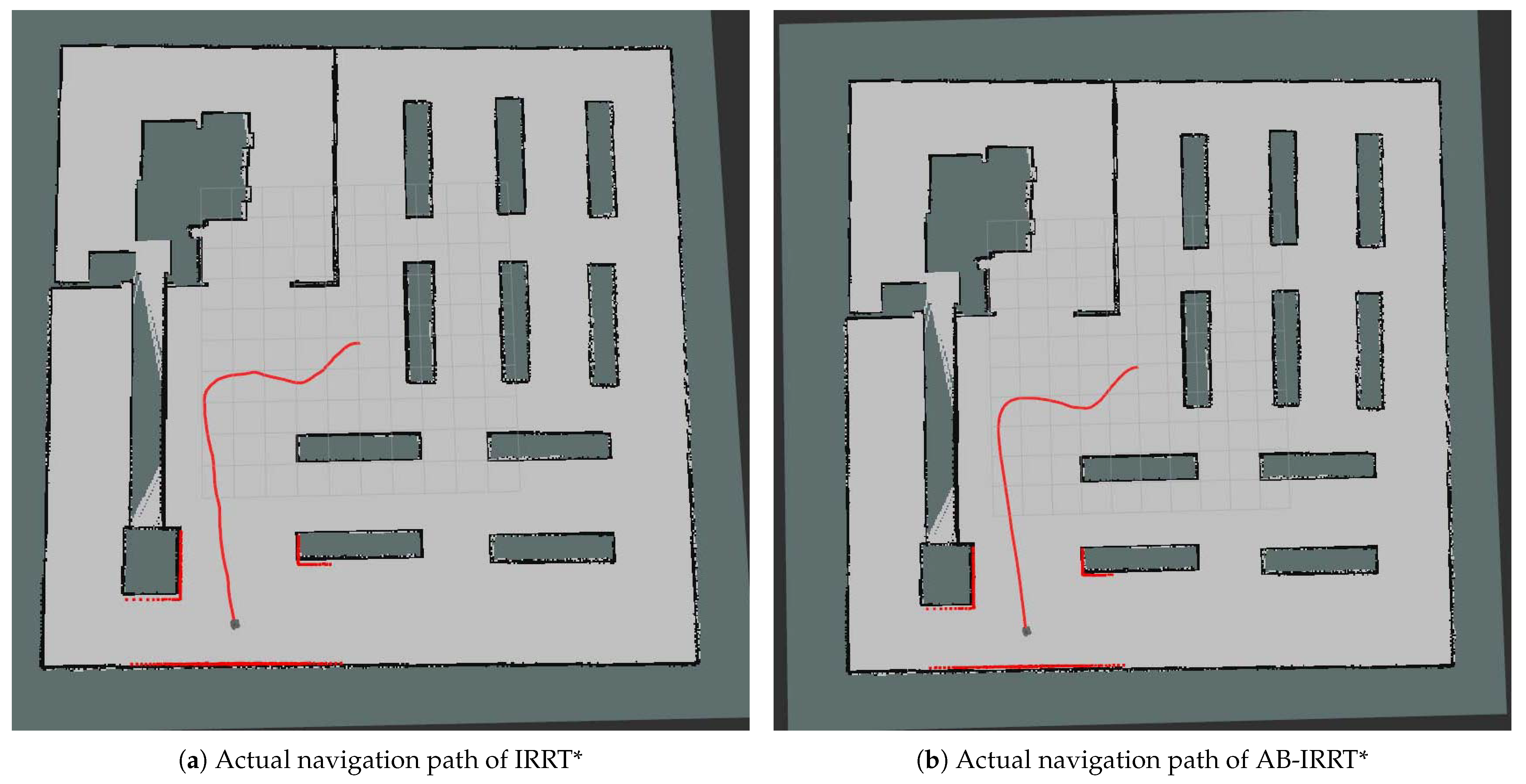
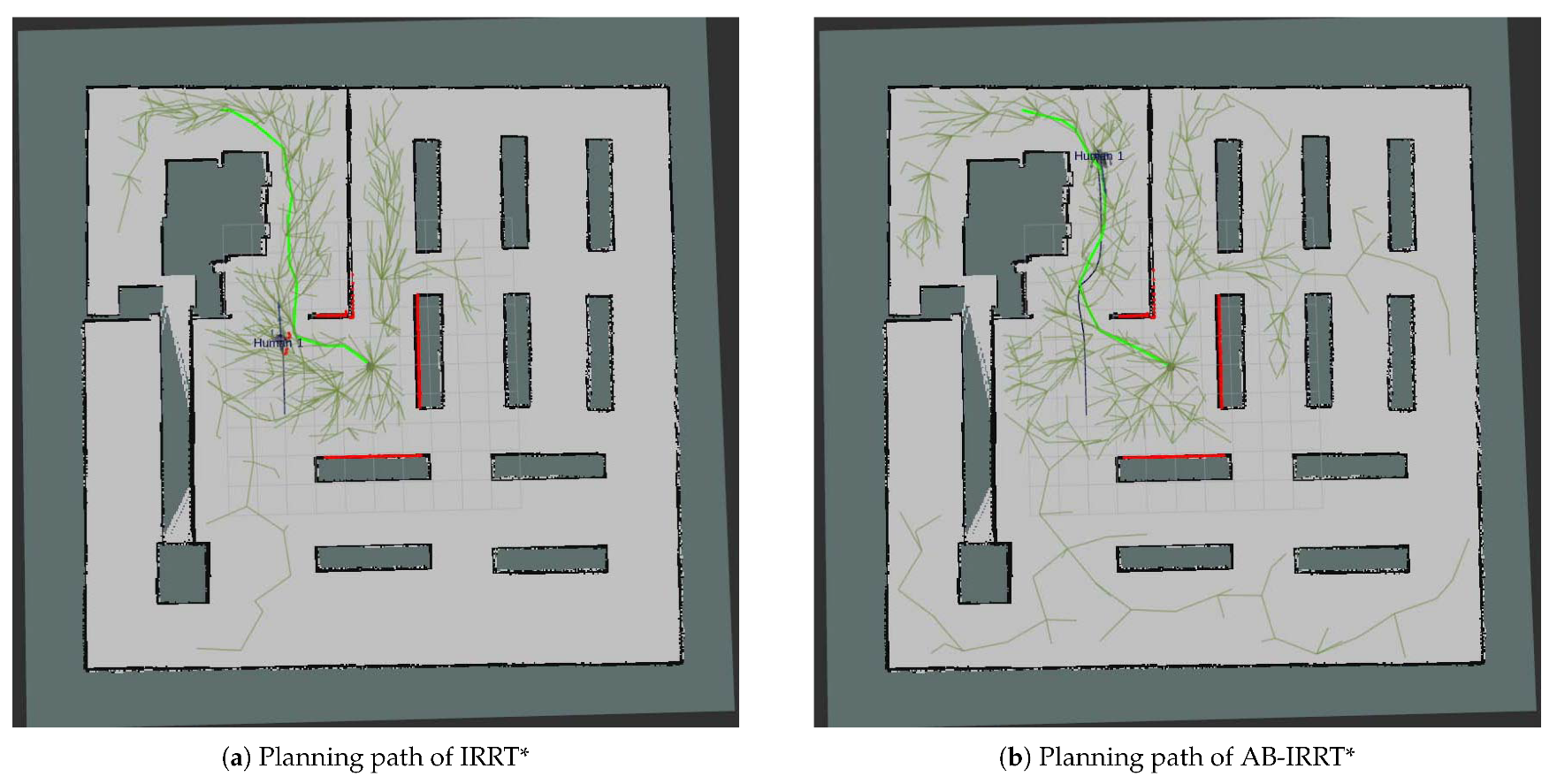
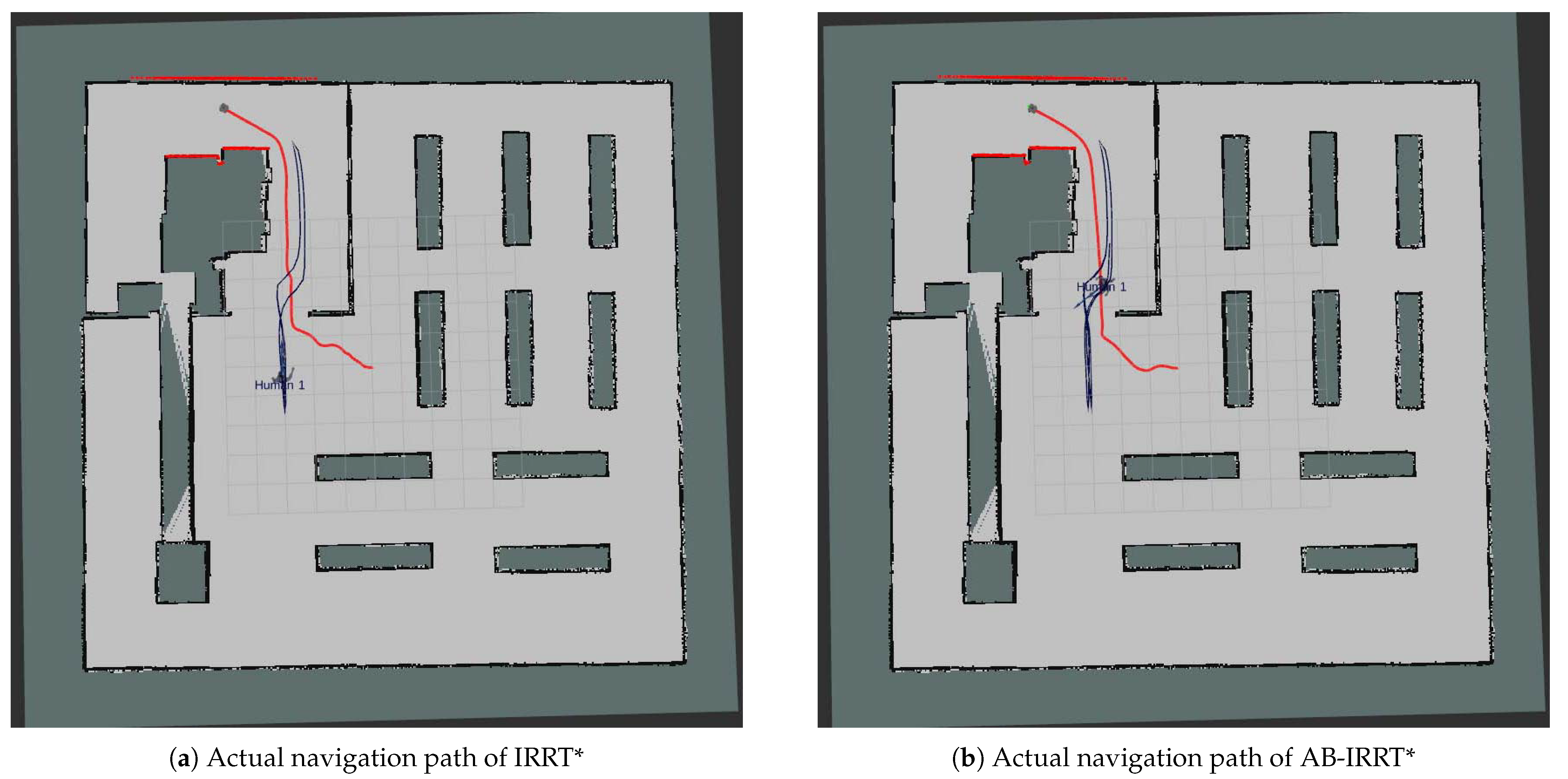
Comparative experiments on six algorithms across three different environments reveal that Strategies A and B each have distinct advantages in generating initial solutions and improving algorithm efficiency. Strategy A performs better in environments with irregular obstacles, while Strategy B is more effective in environments with regular obstacles. When combined, the two strategies enhance the algorithm’s robustness and adaptability across different environments. A subsequent analysis of the computational resource usage of the proposed algorithm shows that the combination of Strategies A and B leads to only a slight increase in CPU and memory usage. In comparison to the performance improvements, this slight increase in resource consumption is entirely acceptable. Finally, navigation experiments were conducted in a simulated environment with unknown and dynamic obstacles. The experimental results show that the improved algorithm significantly optimizes both navigation path length and time, thereby reducing the robot’s energy consumption during navigation. Furthermore, the experiments indicate that the improved algorithm generates smoother navigation paths, further highlighting its superior robustness and real-time performance in complex environments.