Identification and Localization Study of Grounding System Defects in Cross-Bonded Cables

Abstract

Cross-bonded cables improve transmission efficiency by optimizing the grounding method. However, due to the complexity of their grounding system, they are prone to multiple types of defects, making defect state identification more challenging. Additionally, accurately locating sheath damage defects becomes more difficult in cases of high transition resistance. To address these issues, this paper constructs a distributed parameter circuit model for cross-bonded cables and proposes a particle swarm optimization support vector machine (PSO-SVM) defect classification model based on the sheath voltage and current phase angle and amplitude characteristics. This model effectively classifies 25 types of grounding system states. Furthermore, for two types of defects—open joints and sheath damage short circuits—this paper proposes an accurate segment-based location method based on fault impedance characteristics, using zero-crossing problems to achieve efficient localization. The results show that the distributed parameter circuit model for cross-bonded cables is feasible for simulating electrical quantities, as confirmed by both simulation and real-world applications. The defect classification model achieves an accuracy of over 97%. Under low transition resistance, the defect localization accuracy exceeds 95.4%, and the localization performance is significantly improved under high transition resistance. Additionally, the defect localization method is more sensitive to variations in cable segment length and grounding resistance impedance but less affected by fluctuations in core voltage and current.

1. Introduction

In order to meet the demand for high-power transmission in urban industries, high-voltage cables have been widely used in power systems [1,2,3,4]. However, the operating and laying environment of cables is harsh, and the transport methods such as dragging and wet underground environment can easily lead to grounding system defects such as a breakdown in the outer sheath, moisture in cross-bonded boxes, open joints, and short-circuiting at the joints, which are major safety hazards [5]. The problem of cable grounding system state identification and localization needs to be solved urgently. High-voltage cables are usually single-core structures, and cross-bonded cables reduce the induced voltage in the sheathing loop by interchanging the sheathing or cores between each small segment [6,7,8]. However, the cross-bonded connection design leads to the mutual coupling of sheath information among three phases and complex signal propagation paths in the line, which brings new difficulties in monitoring and diagnosing grounding system defects [9].

At present, the main online monitoring techniques for the condition of HV cables are: the partial discharge monitoring method [10,11,12,13,14], where insulation defects are detected by analyzing the local discharge signals, and methods include image feature extraction, combined with classification algorithms; the dielectric loss method [15,16], where insulation degradation is evaluated by measuring the change in the dielectric loss factor; and the impedance method [17,18], where insulation aging and defects are diagnosed by analyzing impedance changes, and local insulation degradation is detected using methods such as reflection and re-reflection measurements, as well as broadband impedance spectral analysis. However, they all have some significant shortcomings. For example, it is difficult to calculate the leakage current when applying the dielectric loss method in cross-bonded cables [9], and the partial discharge monitoring method relies on high-frequency local discharge sensors at specific locations [19,20,21,22,23,24], which is of limited applicability. On the other hand, the main methods for fault location in HV cables are partial discharge, reflection, and impedance methods. Local discharge pulse signal propagation in the cable shows the characteristics of attenuation under high frequency, and its detection sensitivity is easily interfered with by the complicated electromagnetic environment and actual working conditions [25]. The reflection method is prone to misjudging or ignoring cable defects due to the cross-banded special structure that increases the reflected signal’s attenuation rate and overlap rate between the three phases [26].

The above high-voltage cable fault monitoring and localization methods are mainly aimed at insulation defects in the cable body. However, due to the significant differences in the characteristics of typical grounding system defect types, these methods are not directly applicable to the detection of grounding system defects in cables. Currently, relatively limited research has been conducted on the detection and localization of defects in cross-bonded cable grounding systems, mainly using impedance analysis methods.

The impedance method is generally used in defect classification studies, where an ammeter collects the sheath current of a cable direct grounding box or cross-connection box. The threshold value of the sheath current, the ratio of the sheath current to the core current, and the relative value of the sheath currents of the two terminals of the same sheath loop are used to identify the defects in the grounding system [27]. Massimo Marzinotto and Giovanni Mazzanti [28] present a method for detecting sheath faults by monitoring a threshold value of sheath current at a cross-bonded box. Zhonglei Li et al. [29] established a numerical model to simulate the sheath current of cross-linked cables. They also looked at how the sheath current of coaxial cables changes when there are different defects and suggested a way to figure out what kind of defects there are by comparing the fault’s size to the expected amplitude of the current. Xiang Dong et al. [30] developed a cable circuit model for cross-bonded grounded systems to calculate the sheath currents. It analyzed the sheath currents under three typical defects, i.e., open joints, short-circuited joints with breakdowns, and short-circuited cross-bonded boxes. Yilin Wang et al. [31] suggested that the ratio of the sheath current to the core current at the moment of the daily maximum load current should be used as a characteristic value for evaluating the grounding state, considering how the sheath current and core current change over time. Qingzhu Wan and Xuyang Yan [32] suggested a way to get 14-dimensional features by comparing the size and phase of the 6-phase current data gathered at the cross-bonded box. Machine-learning algorithms could then use these features to identify issues in the grounding system. This reference classifies the defect types according to the circuit’s topology, which can effectively identify typical defects in multiple categories of grounding systems. However, constructing the sample library for the defect classification model in that reference is based on an imperfect cable model that ignores the electromagnetic induction component of the core leakage current on the sheath. Therefore, the method is flawed in calculating the characteristic current samples themselves, which makes the logic and accuracy of the defect judgment model suffer. The cable model constructed for defect classification in the above references is a double-π model that considers the electromagnetic and electrostatic coupling between the core and the sheath. However, it can only calculate the sheath’s voltages and currents at the cross-bonded box and the direct grounding box, and it cannot efficiently locate defects such as sheath breakdowns and grounding short circuits.

Impedance methods for grounding system defects localization research, such as Mirko Todorovski and Risto Ackovski [33], built a two-layer impedance model of high-voltage cables based on the electrical quantity time domain analysis method to establish the core-sheath short-circuit fault equations to locate the fault location. Chengjun Xia et al. [34] used impedance and conductance matrix to represent the coupling between the core and sheath and constructed a π-type equivalent model of distributed electrical quantities to simulate along the cross-bonded cables. A distance measurement equation is established based on this circuit model and the characteristics of the electrical quantities at the fault location, but the accuracy of the distance measurement is affected by high-transition resistance. The cable models used in the aforementioned defect location studies are lumped parameter models, which do not consider the impact of the distributed capacitance of the cable on the sheath conductor. Wenxia Pan et al. [35] proposed a distributed parameter model that does not consider the higher-order terms of infinitesimal segments to detect insulation faults in cross-bonded cables. Jian Luo et al. [36] proposed a circuit model of line distribution characteristics considering higher-order terms of infinitesimal segments, which can calculate the lines’ electrical signals. However, the model only applies to single-phase transmission lines and is not applicable to actual three-phase cables.

Therefore, the above-mentioned studies have two main issues. First, the circuit model for cross-bonded cables in defect identification research has not been fully established. The model does not sufficiently account for the coupling factors between the core and the sheath. Secondly, after defect identification, the location of the sheath damage point has not been determined. Furthermore, traditional defect location models are lumped parameter models, which do not consider the effects of distributed capacitance. Also, not much research has been done on problems in the cross-bonded cable grounding system, and it is not very accurate to find outer-sheath breakdown defects when the transition resistance is high.

In response to the shortcomings of traditional cable models and grounding system defect identification and location methods, the main research of this paper is to construct an equivalent model of the cross-bonded cable loop and, based on this, propose a diagnostic method based on the electrical characteristic quantities of the sheath. The Particle Swarm Optimized Support Vector Machine (PSO-SVM) classification algorithm is effective in identifying the type of grounding system state of cross-bonded cables. In addition, for the defect localization of two types of defects, namely, open joints and short circuits with sheath breakdown grounding, a method based on fault impedance characteristics is adopted to transform the problem into a zero-point problem. Then, a defect localization method is derived, and the feasibility of the method is verified by simulation.

2. Cross-Bonded Cable Distribution Parameter Model

2.1. Model Theory

A structural diagram of a cross-bonded main section is shown in Figure 1, and the metal sheath is swapped between the cross-bonded boxes J1 and J2. jxy (x = A, B, C, y = 0, 1, 2, 3) denotes the metallic joints, and A1–C3 represents the main section of the cross-bonded cable, which is divided into nine smaller segments. The sensors are mounted on the cable core and sheath and are used to collect the voltage and current at the beginning terminal and terminal.

Cross-bonded cables usually use single-core cables with two metal conductors: a core and a metal sheath. The team previously derived and verified the transmission line distribution parameter model [35], based on which this paper derives the distribution parameter model of cross-bonded cables. Because the focus of this paper is to conduct the detection and localization study of cable grounding system defects based on the model, the correct derivation of the model is provided directly in Equation (1).

In Figure 2, $u_{\mathrm{cM}}(t)$, $u_{\mathrm{sM}}(t)$, $i_{\mathrm{cM}}(t)$, $i_{\mathrm{sM}}(t)$ and $u_{\mathrm{cN}}(t)$, $u_{\mathrm{sN}}(t)$, $i_{\mathrm{cN}}(t)$, $i_{\mathrm{sN}}(t)$ show the voltages and currents at the core and the sheath’s beginning and ending terminals at time $t$, respectively. $R_{\mathrm{c}}$, $R_{\mathrm{s}}$, $L_{\mathrm{c}}$, $L_{\mathrm{s}}$ and $R_m$, $M_m$ are the unit self-resistance, self-inductance, mutual resistance, and mutual inductance of the core and sheath of the cable, respectively. $C_{\mathrm{cs}}$ and $C_{\mathrm{sg}}$ indicate the equivalent capacitance of the main insulation and the unit equivalent capacitance of the insulation between the sheath and the ground. Point $k_1$ is at a distance of $l$ from terminal $M$. $i_{\mathrm{c}}(x,t)$, $u_{\mathrm{c}}(x,t)$ and $i_{\mathrm{s}}(x,t)$, $u_{\mathrm{s}}(x,t)$ are the currents and voltages in the core and sheath at point $k_1$ in time $t$, respectively.

$$\begin{array}{l}\left\{\begin{array}{l}{u}_{\mathrm{c}\mathrm{N}}(t)=u_{\mathrm{c}\mathrm{M}}(t)-[R_{\mathrm{c}}{i}_{\mathrm{c}\mathrm{M}}(t)+L_{\mathrm{c}}{\displaystyle \frac{d{i}_{\mathrm{c}\mathrm{M}}(t)}{dt}}+R_{\mathrm{m}}{i}_{\mathrm{s}\mathrm{M}}(x,t)+M_{\mathrm{m}}{\displaystyle \frac{d{i}_{\mathrm{s}\mathrm{M}}(t)}{dt}}]l+{\displaystyle \sum _{j=1}^{\infty }{P}_{\mathrm{c}\mathrm{n}}(j)}\\ i_{\mathrm{c}\mathrm{N}}(t)=i_{\mathrm{c}\mathrm{M}}(t)+{\displaystyle \sum _{j=1}^{\infty }{Q}_{\mathrm{c}\mathrm{n}}(j)}\end{array}\right.\\ \left\{\begin{array}{l}{u}_{\mathrm{s}\mathrm{N}}(t)=u_{\mathrm{s}\mathrm{M}}(t)-[R_{\mathrm{s}}{i}_{\mathrm{s}\mathrm{M}}(t)+L_{\mathrm{s}}{\displaystyle \frac{\partial i_{\mathrm{s}\mathrm{M}}(t)}{dt}}+R_{\mathrm{m}}{i}_{\mathrm{c}\mathrm{M}}(t)+M_{\mathrm{m}}{\displaystyle \frac{d{i}_{\mathrm{c}\mathrm{M}}(t)}{dt}}]l+{\displaystyle \sum _{j=1}^{\infty }{P}_{\mathrm{s}\mathrm{n}}(j)}\\ i_{\mathrm{s}\mathrm{N}}(t)=i_{\mathrm{s}\mathrm{M}}(t)+{\displaystyle \sum _{j=1}^{\infty }{Q}_{\mathrm{s}\mathrm{n}}(j)}\end{array}\right.\end{array}$$

(1)

where: $P_{\mathrm{c}\mathrm{n}}$, $P_{\mathrm{s}\mathrm{n}}$, $Q_{\mathrm{c}\mathrm{n}}$, and $Q_{\mathrm{s}\mathrm{n}}$ are polynomials on $R_{\mathrm{c}}$, $L_{\mathrm{c}}$, $R_{\mathrm{s}}$, $L_{\mathrm{s}}$, $R_{\mathrm{m}}$, $C_{\mathrm{cs}}$, $C_{\mathrm{sg}}$, $M_{\mathrm{m}}$, and $△x^{\mathrm{k}}$ (k = 0, 1, 2, 3, …), the details of which will not be repeated. u and i denote voltage and current, and R, L, and M denote the electrical parameters of the cable, described in detail as described in rows 156–163. Ultimately, through the mathematical induction method, the method of coefficients to be determined, and the recursive method, the relationship between the electrical quantity at the ending terminal of the cable and the beginning terminal can be obtained. As a result, in the known single-phase cable basic parameters and the electrical quantity of the beginning terminal core and sheath at $t$ time, the use of Formula (1) can be obtained at $t$ time for the electrical quantity of the single-phase cable-ending terminal core and sheath.

According to IEEE, the equilateral triangle arrangement can best eliminate the phase-to-phase induced voltage and reduce the sheath current under the same conditions, and it is a common arrangement in high-voltage power systems. It is assumed that the three-phase cables of the equilateral triangular arrangement are the same type, and the phase-to-phase impedance is approximately the same. Figure 3 shows the inter-phase coupling relationship of the cross-bonded cable in a certain infinitesimal segment. In the figure, core self-impedance is $Z\mathrm{cc}$, sheath self-impedance is $Z\mathrm{ss}$, the mutual impedance of the interactions between the core and the sheath is named as $Z\mathrm{cs}$, and the phase-to-phase mutual impedance is ${Z\prime }_{\mathrm{CS}}$. To obtain the distribution parameter model, these characteristics can be used in three-phase cables to eliminate the phase-to-phase coupling relationship, i.e., to eliminate the phase-to-phase mutual impedance ${Z\prime }_{\mathrm{CS}}$.

$Z$ is the three-phase unit impedance matrix for any portion of the cross-bonded cable:

$$Z=\left(\begin{array}{cccccc}Z\mathrm{cc}& {Z^{\prime }}_{\mathrm{CS}}& {Z^{\prime }}_{\mathrm{CS}}& Z\mathrm{cs}& {Z^{\prime }}_{\mathrm{CS}}& {Z^{\prime }}_{\mathrm{CS}}\\ {Z^{\prime }}_{\mathrm{CS}}& Z\mathrm{cc}& {Z^{\prime }}_{\mathrm{CS}}& {Z^{\prime }}_{\mathrm{CS}}& Z\mathrm{cs}& {Z^{\prime }}_{\mathrm{CS}}\\ {Z^{\prime }}_{\mathrm{CS}}& {Z^{\prime }}_{\mathrm{CS}}& Z\mathrm{cc}& {Z^{\prime }}_{\mathrm{CS}}& {Z^{\prime }}_{\mathrm{CS}}& Z\mathrm{cs}\\ Z\mathrm{cs}& {Z^{\prime }}_{\mathrm{CS}}& {Z^{\prime }}_{\mathrm{CS}}& Z\mathrm{ss}& {Z^{\prime }}_{\mathrm{CS}}& {Z^{\prime }}_{\mathrm{CS}}\\ {Z^{\prime }}_{\mathrm{CS}}& Z\mathrm{cs}& {Z^{\prime }}_{\mathrm{CS}}& {Z^{\prime }}_{\mathrm{CS}}& Z\mathrm{ss}& {Z^{\prime }}_{\mathrm{CS}}\\ {Z^{\prime }}_{\mathrm{CS}}& {Z^{\prime }}_{\mathrm{CS}}& Z\mathrm{cs}& {Z^{\prime }}_{\mathrm{CS}}& {Z^{\prime }}_{\mathrm{CS}}& Z\mathrm{ss}\end{array}\right)$$

(2)

The symmetric component method is applied to the phase-mode transformation of transmission lines, which can eliminate the mutual inductive coupling in the network equations of the system. A decoupling matrix $P$ after the extension of the above method is proposed:

$$P=\left(\begin{array}{cccccc}1& 1& 1& 0& 0& 0\\ s^2& s& 1& 0& 0& 0\\ s& s^2& 1& 0& 0& 0\\ 0& 0& 0& 1& 1& 1\\ 0& 0& 0& s^2& s& 1\\ 0& 0& 0& s& s^2& 1\end{array}\right)$$

(3)

Of which $s=-{\displaystyle \frac{1}{2}}+j{\displaystyle \frac{\sqrt{3}}{2}}$.

$$\begin{array}{l}{u}_{\mathrm{mod}}=P^{-1}{u}_{\mathrm{ABC}}, u_{\mathrm{ABC}}=P{u}_{\mathrm{mod}}\\ i_{\mathrm{mod}}=P^{-1}{i}_{\mathrm{ABC}},i_{\mathrm{ABC}}=P{i}_{\mathrm{mod}}\end{array}$$

(4)

$$Z_{\mathrm{mod}}=P^{-1}ZP$$

(5)

$$Z_{\mathrm{mod}}=\left[\begin{array}{cccccc}{Z}_{\mathrm{C}1}& & & Z_{\mathrm{CS}1}& & \\ & Z_{\mathrm{C}2}& & & Z_{\mathrm{CS}2}& \\ & & Z_{\mathrm{C}3}& & & Z_{\mathrm{CS}3}\\ Z_{\mathrm{CS}1}& & & Z_{\mathrm{S}1}& & \\ & Z_{\mathrm{CS}2}& & & Z_{\mathrm{S}2}& \\ & & Z_{\mathrm{CS}3}& & & Z_{\mathrm{S}3}\end{array}\right]$$

(6)

$$u_{\mathrm{ABC}}=\left[\begin{array}{c}{u}_{\mathrm{CA}}\\ u_{\mathrm{CB}}\\ u_{\mathrm{CC}}\\ u_{\mathrm{SA}}\\ u_{\mathrm{SB}}\\ u_{\mathrm{SC}}\end{array}\right]; i_{\mathrm{ABC}}=\left[\begin{array}{c}{i}_{\mathrm{CA}}\\ i_{\mathrm{CB}}\\ i_{\mathrm{CC}}\\ i_{\mathrm{SA}}\\ i_{\mathrm{SB}}\\ i_{\mathrm{SC}}\end{array}\right]; u_{\mathrm{mod}}=\left[\begin{array}{c}{u}_{\mathrm{C}1}\\ u_{\mathrm{C}2}\\ u_{\mathrm{C}3}\\ u_{\mathrm{S}1}\\ u_{\mathrm{S}2}\\ u_{\mathrm{S}3}\end{array}\right]; i_{\mathrm{mod}}=\left[\begin{array}{c}{i}_{\mathrm{C}1}\\ i_{\mathrm{C}2}\\ i_{\mathrm{C}3}\\ i_{\mathrm{S}1}\\ i_{\mathrm{S}2}\\ i_{\mathrm{S}3}\end{array}\right]$$

(7)

$u_{\mathrm{ABC}}$ and $i_{\mathrm{ABC}}$ are the three-phase cable voltage and current phasors, $u_{\mathrm{mod}}$ and $i_{\mathrm{mod}}$ are the modulus, and the elements in $Z_{\mathrm{mod}}$ are the decoupled modal impedance matrix. The symmetric phase impedance matrix $Z$ is decoupled by the asymmetric decoupling matrix $P$ to obtain the modal impedance matrix $Z_{\mathrm{mod}}$ with symmetry. After decoupling $Z_{\mathrm{mod}}$, the element at position $Z$ in ${Z\prime }_{\mathrm{CS}}$ becomes 0. In the modal domain, the interphase modulus is independent of each other. A coupling relationship still exists between the in-phase core and sheath modulus, corresponding to the cable single-phase distribution parameter model in Equation (1). Knowing the basic parameters of the three-phase cable, as well as the electrical quantities of the core and sheath at the first (last) terminal at time $t$, the phase quantities are first converted to a modulus using the first partition of the voltage and current transformations of Equation (4). Then, the decoupling matrix is decoupled using Equation (5). Finally, by combining Equation (1), the electrical quantities of the core and sheath at the end (first) terminal of the three-phase cable at time $t$ can be calculated.

After transformation and calculation, the electrical quantity obtained is the modulus at the ending terminal of a segment. For cross-bonded cables, the electrical quantity for each segment is calculated segment by segment as described above. For each segment, the modulus at the ending terminal of the previous segment is calculated, and then the modulus phase mode is inversely transformed into a phase quantity utilizing the second partition of the voltage and current transformations of Equation (4). The data for the beginning terminal of the next segment are obtained by keeping the order of the core electrical quantities unchanged and transposing the order of the sheath electrical quantities. In this way, by analogy, the electrical quantities of the core and sheath at the ending of the cross-bonded cable at time $t$ can be obtained. To obtain the three-phase cable, with the beginning terminal $u_{\mathrm{ABC}}^{\mathrm{M}}$, $i_{\mathrm{ABC}}^{\mathrm{M}}$ and the ending terminal $u_{\mathrm{ABC}}^{\mathrm{N}}$, $i_{\mathrm{ABC}}^{\mathrm{N}}$, the function relationship is as follows, with $l$ for the cable length:

$$\begin{array}{l}(u_{\mathrm{ABC}}^{{\mathrm{N}\prime }_{\mathrm{S}}},i_{\mathrm{ABC}}^{{\mathrm{N}\prime }_{\mathrm{S}}},u_{\mathrm{ABC}}^{{\mathrm{N}\prime }_{\mathrm{C}}},i_{\mathrm{ABC}}^{{\mathrm{N}\prime }_{\mathrm{C}}})=f(u_{\mathrm{ABC}}^{\mathrm{M}},i_{\mathrm{ABC}}^{\mathrm{M}},l)\\ (u_{\mathrm{ABC}}^{{\mathrm{M}\prime }_{\mathrm{S}}},i_{\mathrm{ABC}}^{{\mathrm{M}\prime }_{\mathrm{S}}},u_{\mathrm{ABC}}^{{\mathrm{M}\prime }_{\mathrm{C}}},i_{\mathrm{ABC}}^{{\mathrm{M}\prime }_{\mathrm{C}}})=f(u_{\mathrm{ABC}}^{\mathrm{N}},i_{\mathrm{ABC}}^{\mathrm{N}},l)\end{array}$$

(8)

2.2. Model Validation

2.2.1. Simulation Verification

To verify the correctness of the distributed parameter model proposed in Section 2.1, a simulation model of the cross-bonded cable main section was established using the ATP-EMTP simulation platform. A 220 kV sinusoidal voltage is used to power the system. The cables used are YJLW03-127/220-1 × 2000, which are arranged in an equilateral triangle manner, with phase A and phase C at the same height from the ground. The beginning terminal sheathing is grounded by a 0.01 Ω resistance, and a 1 Ω resistance grounds the ending terminal sheathing. The sampling frequency is 1 kHz. The U and I of the cores and sheaths at the beginning terminal of the cable were collected and coded into the distribution parameter model using MATLAB 2023b. The U and I of the cable core and sheath at the terminal were calculated by inputting the collected U and I data of the beginning terminal into the model code.

The results of the simulation and calculation of the comparison cross-bonded cable ending terminal are shown in Figure 4. The relative error is calculated using Equation (9), where $compute{d}_i$ denotes the calculated value at a sampling point $i$ and $sample{d}_i$ denotes the sampling value at a sampling point $i$ of the simulation. The sampling duration of this experiment is 0.02 s with 21 sampling points, i.e., $N$ = 21.

$$RE={\displaystyle \frac{{\displaystyle \sum _{i=1}^N\left|\frac{ compute{d}_i - sample{d}_i}{sample{d}_i}\right|}}{N}}\times 100$$

(9)

The relative errors of the three-phase core voltages are not more than 0.017%, the core currents are less than 0.0013%, and those of the sheathing currents are less than 0.54%. The above discrepancy data verify the correctness of the model.

2.2.2. Practical Verification

The proposed model is applied to a normal-running 220 kV cross-bonded cable in Chongqing, which is laid in a cable trench, and no grounding system abnormality, etc., has occurred until the experiment. This cable consists of a complete cross-bonded main section. The cable model is also a YJLW03-127/220-1 × 2000-type cable, arranged in a positive triangle, with phase A parallel to phase C and a height of 0.1 m from the ground level.

The fault recorder at the substation cannot only be activated when the line is faulted but also can be turned on manually, and both of them can record the three-phase currents in the line and the corresponding three-phase voltage waveforms of the busbar. In this experiment, the fault recorder is manually turned on at the substation to collect the U and I at the beginning terminal of the core, with a sampling frequency of 4 kHz and millisecond precision at the substation. In the cable, two direct grounding lines have access to flexible current sensors, a sampling frequency of 5 kHz, and a time accuracy of ± 100 ns. The two direct grounding box B-phase core currents and three-phase sheath currents (measured to the cable at both ends of the sheath voltage order of magnitude of millivolts, approximated to 0 V) are synchronized through the GPS synchronization equipment. The currents collected by the current sensor are the sheath currents at the beginning terminal and ending terminal of the cable and the B-phase core current. Figure 5 displays the substation line core electrical signal acquisition device, along with the grounding system sheath electrical signal synchronization acquisition device and measurement diagram.

To further minimize asynchronous errors in core and sheath measurements, the relative time between the phase B core current collected by the sheath measurement system and the peak point of the phase B core current collected by the core measurement system was used as the moving time of the other collected quantities of the core. The adaptive filtering method is used to filter the collected beginning terminal data. The A-phase sheath current can be used as an example, while the comparison graph before and after filtering is shown in Figure 6a. The three-phase sheath currents at the terminal are calculated using the cross-bonded cable distribution parameter model in Section 2.1, and the comparison between the actual measured and calculated values at the terminal is shown in Figure 6b. Under ideal operation conditions without defects in the grounding system, the sheath current is offset by three-phase sheath cross-interconnection. However, there are unavoidable situations in practice: (1) Cables arranged in positive triangles in order to transpose the sheath in the cross-connected interconnection box need to lead the sheath conductor through the coaxial cable in advance, and the coaxial cable at the coaxial cable is generally used in the form of a linear arrangement; (2) in one cross-bonded main section, multiple small cables are in a cross-bonded main segment, the length distribution of multiple small segments is unbalanced, and the induced current cannot be completely canceled. The average error of the three-phase terminal sheath current is 0.3164 A for phase A, 0.3415 A for phase B, and 0.3351 A for phase C, and the total average error is 0.3310 A, which is within the permissible range of actual working conditions. There is still a particular gap between the calculated and measured values, mainly because the engineering site is often more complex, and there are usually simplified parameters when calculating.

3. Grounding System Defect Identification

3.1. Classification and Simulation of Grounding System Defects

Reference [32] summarizes four common defects in cross-bonded cable grounding systems: open circuit defects caused by loose sheath protectors, short circuit defects between sheath loops caused by joint breakdown, ground short circuit defects due to moisture in the cross-bonding box, and ground short circuit defects caused by damage to the outer sheath. This paper divides these defects into three major categories according to the circuit topology; see

Table 1. Classification of cross-bonded cable grounding system states.

Circuit Topology	Defect Summary	Defect Location	Status Number
Normal circuit			25
Sheath loop Open circuit	Sheathing loop 1 (A1-B2-C3) open circuit	Joints JA0, JA1, JB1, JB2, JC2, JC3	01
	Sheathing loop 2 (B1-C2-A3) open circuit	Joints JB0, JB1, JC1, JC2, JA2, JA3	02
	Sheathing loop 3 (C1-A2-B3) open circuit	Joints JC0, JC1, JA1, JA2, JB2, JB3	03
Short circuit between sheathing circuits	Between sheaths (A1-A2)	Joint JA1	04
	Between sheaths (B1-B2)	Joint JB1	05
	Between sheaths (C1-C2)	Joint JC1	06
	Between sheaths (A2-A3)	Joint JA2	07
	Between sheaths (B2-B3)	Joint JB2	08
	Between sheaths (C2-C3)	Joint JC2	09
Sheathed circuits shorted to ground Cross-bonded box dampness	A1-B2 protector short circuit	Cross-bonding Box CB1	10
	B1-C2 protector short circuit	Cross-bonding Box CB1	11
	A1-C2 protector short circuit	Cross-bonding Box CB1	12
	A2-B3 protector short circuit	Cross-bonding Box CB2	13
	B2-C3 protector short circuit	Cross-bonding Box CB2	14
	C2-A3 protector short circuit	Cross-bonding Box CB2	15
Sheathed circuits shorted to ground Sheath broken	Segment A1	Segment A1	16
	Segment B1	Segment B1	17
	Segment C1	Segment C1	18
	Segment A2	Segment A2	19
	Segment B2	Segment B2	20
	Segment C2	Segment C2	21
	Segment A3	Segment A3	22
	Segment B3	Segment B3	23
	Segment C3	Segment C3	24

.

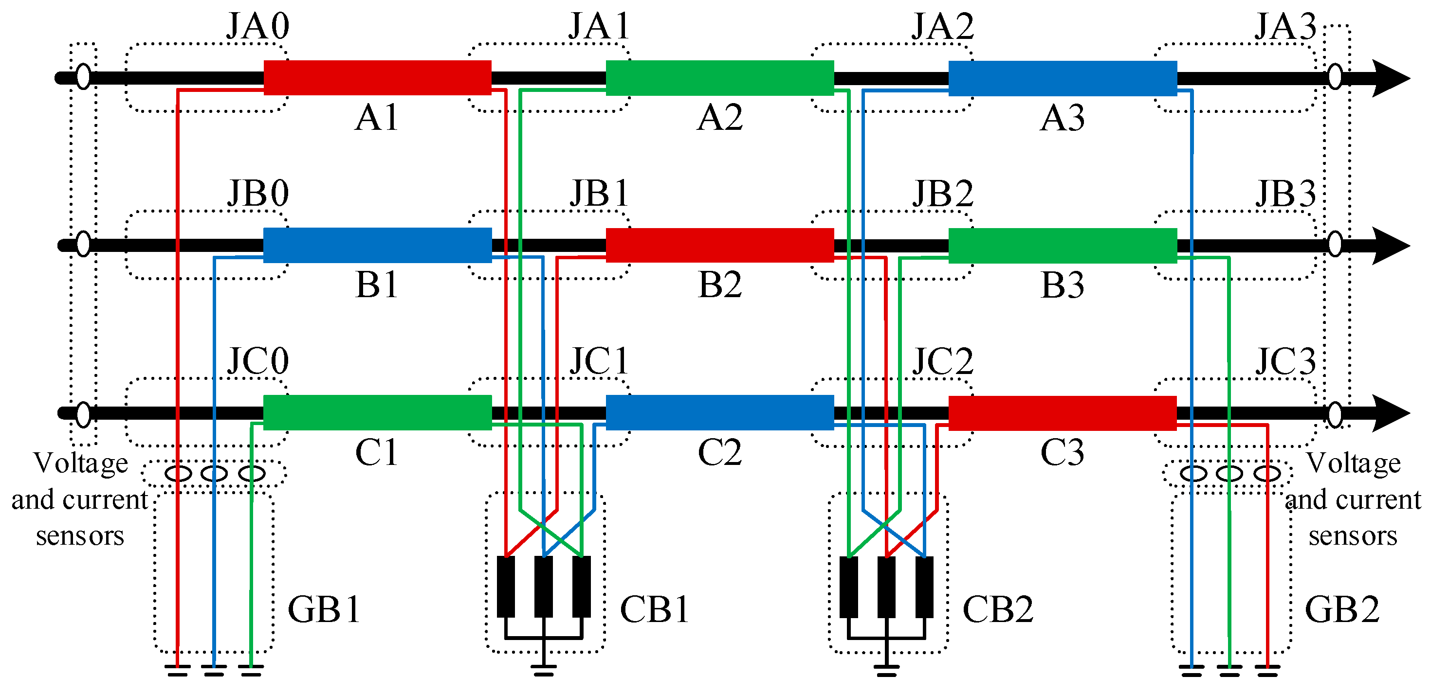
Twenty-four grounding system defects are simulated in the simulation by changing the cable grounding system connection structure or adding a branch circuit to the ground, as shown in Figure 7, and examples of the defect simulation modes are as follows: (A) sheath loop open-circuit defects (a1): junction JA0 disconnecting the grounding lead; (B) sheath circuit inter-circuit short-circuit defect (b1): shorting of the metal sheath at junction JA1; (C) protector short circuit to ground defect (c1): failure of protector in cross-bonded box CB1 resulting in low resistance grounding; (D) additional short circuit to ground defect with breakdown in the outer sheath (d1): additional branch circuit to ground with breakdown in the sheath at segment A1.

3.2. Selection of Sheath Current and Voltage Characteristics

When the cable grounding system is in normal operation, the equivalent circuit model from the cable terminal of the current and voltage values calculated from the other terminal of the current and voltage values and sampling values are basically equal. When the cable grounding system is defective due to the impact of the fault loop, the cable, M to N, of the equivalent circuit model is destroyed. Then, the electrical quantities at both terminals of the cable are collected. Based on the sampled values of core and sheath electrical quantities at M (N), the calculated values of sheath current and voltage at N (M) are obtained after equivalent circuit modeling, and the difference between the sampled and calculated values at N (M) is observed.

To select the eigenvalue that can effectively identify the information on the type of defects in the grounding system, the information on the magnitude and phase angle of the sheath currents and voltages that react differently in different defect states are included, and the eigenvalues are calculated as the relative difference between the calculated values of the magnitude of the voltage and current of the sheaths at the end of the cables, ${U\prime }_{\mathrm{i}}$, ${I\prime }_{\mathrm{i}}$, and the sampled values, U_i, I_i, which are calculated as the absolute differences between the calculated values of the phase of the electrical quantities of the sheaths at the end ${\mathsf{\phi }}_{\mathrm{Ui}}^{\prime }$, ${\mathsf{\phi }}_{\mathrm{Ii}}^{\prime }$, and the sampled values ${\mathsf{\phi }}_{\mathrm{Ui}}$, ${\mathsf{\phi }}_{\mathrm{Ii}}$. This constitutes a 12-dimensional characteristic phase $[x_1,x_2,\dots x_{12}]$, for example, $x_1=(U_{\mathrm{A}}-U_{\mathrm{A}}^{\prime })/U_{\mathrm{A}}^{\prime }$, $x_7={\mathsf{\phi }}_{\mathrm{IA}}-{\mathsf{\phi }}_{\mathrm{IA}}^{\prime }$.

To obtain a large number of datasets, considering the complexity of the cable operating environment and the diversity of laying methods, the basic parameters, such as the cable structure, should be kept unchanged while randomly adjusting the length of the cable segments (400–600 m), the distance between phases (0.1–0.3 m), the load impedance (200–660 Ω), and the transition resistance (0.01–100 Ω) and other variables in the process of the feature calculation. The 25 states of the grounding system in Table 1 are set up with simulation parameters according to the structural parameters of the YJLW03-121/220-1 × 2000 model cable and the four random parameters mentioned above, and 814 feature samples are generated for each category, which results in a total of 20,350 feature samples, with 12 voltage and current eigenvalues contained in each set of data. The dataset is randomly split into a training set and a testing set with a ratio of 1:4.

3.3. Defect Identification Model Based on PSO-SVM

3.3.1. Support Vector Machines

Support Vector Machine (SVM) separates data by constructing an optimal classification hyperplane $w^{T}x+b=0$ [37]. This hyperplane satisfies the following constraints:

$$\underset{w,b,\xi }{\min }{\displaystyle \frac{1}{2}}\Vert w{\Vert }^2+C{\displaystyle \sum _{i=1}^n{\xi }_i}$$

(10)

$$\mathrm{s}.\mathrm{t}. y_i(w^T{x}_i+b)\ge 1-{\xi }_i, {\xi }_i\ge 0 i=1,2,\dots ,n$$

(11)

In the formula, $w$ corresponds to the weight vector, $b$ is the bias, ${\xi }_i$ refers to the slack variables, and $C$ is the regularization parameter.

Constructing the hyperplane is equivalent to solving the constrained quadratic programming problem. After solving, the decision function obtained is:

$$y(x)=\mathrm{sgn}\left[{\displaystyle \sum _{i=1}^n{\alpha }_i}{y}_i(x,x_i)+b\right]$$

(12)

Considering real-world samples are generally non-linearly separable, SVM needs to be combined with kernel methods to transform the low-dimensional non-linearly separable problem into a linearly separable problem in a higher-dimensional space. The decision function in this case is:

$$y(x)=\mathrm{sgn}\left[{\displaystyle \sum _{i=1}^n{\alpha }_i}{y}_{i}K(x,x_i)+b\right]$$

(13)

In the equation, $K(x,x_i)$ represents the kernel function. In this paper, the more flexible and widely applied Radial Basis Function (RBF) kernel is used to construct a nonlinear SVM. The RBF kernel is provided by the following Equation (14):

$$K(x,x_i)=\exp \left(-g\Vert x-x_i{\Vert }^2\right)$$

(14)

In the equation, $g$ is the kernel parameter, which is a positive number greater than 0.

3.3.2. Support Vector Machine Recognition Model for Particle Swarm Optimization

The Particle Swarm Optimization (PSO) algorithm starts by randomly initializing particles, then iteratively updates their states to search for the optimal solution, and, finally, identifies the best position based on the discovered optimal solution [38,39].

The procedure for constructing the PSO-SVM identification model is as follows:

Step 1: Set the range for C and $g$ in the SVM model. For this study, the values of C and $g$ are chosen between 0.01 and 100.

Step 2: Define the core parameters of the PSO algorithm. As PSO is sensitive to hyperparameter settings, its optimization results may have certain randomness, leading to fluctuations in classification performance. To reduce this difference, this paper sets the parameter configurations with better results after experimental verification as follows: The local search ability of PSO is initialized to 2, and the global search ability is also set to 2. The maximum number of iterations is initialized at 10, while the swarm size starts at 6. The elasticity coefficient for population updates is set to 1, as is the coefficient for velocity updates.

Step 3: Optimize $C$ and $g$ based on the training data. The adaptation of each generation of particles is evaluated by calculating the mean-square-error function, which is the classification accuracy (objective function) of the SVM. During the calculation process, the classification accuracy is obtained by the 5-fold cross-validation method to evaluate the performance of the model more accurately. Once the fitness of the current generation satisfies the optimal solution conditions (e.g., reaching the target accuracy), output the average fitness, optimal fitness, individual extreme values, and global extreme values, along with the respective $C$ and $g$ values, and move to step 5. If not, continue to step 4.

Step 4: Iteratively optimize C and $g$. Optimize the adaptive changes of the particles, compute the optimal fitness for each iteration, and update the individual and group’s best extrema and positions.

Step 5: Use the C and $g$ parameters optimized by PSO for training the SVM model. Based on the trained classifier, recognition is performed on the test set to evaluate the classification performance of the grounding system defects and validate the model’s accuracy.

3.4. Analysis of Defect State Identification Results

In order to evaluate the performance of the classification model in distinguishing between different grounding system states, the metric of recognition accuracy is proposed and calculated as Equation (15):

$$A={\displaystyle \frac{TP+TN}{P+N}}$$

(15)

TP (True Positive) represents the number of samples correctly categorized as positive. TN (True Negative) represents the number of samples correctly categorized as negative. p represents all positive cases. n represents all negative cases.

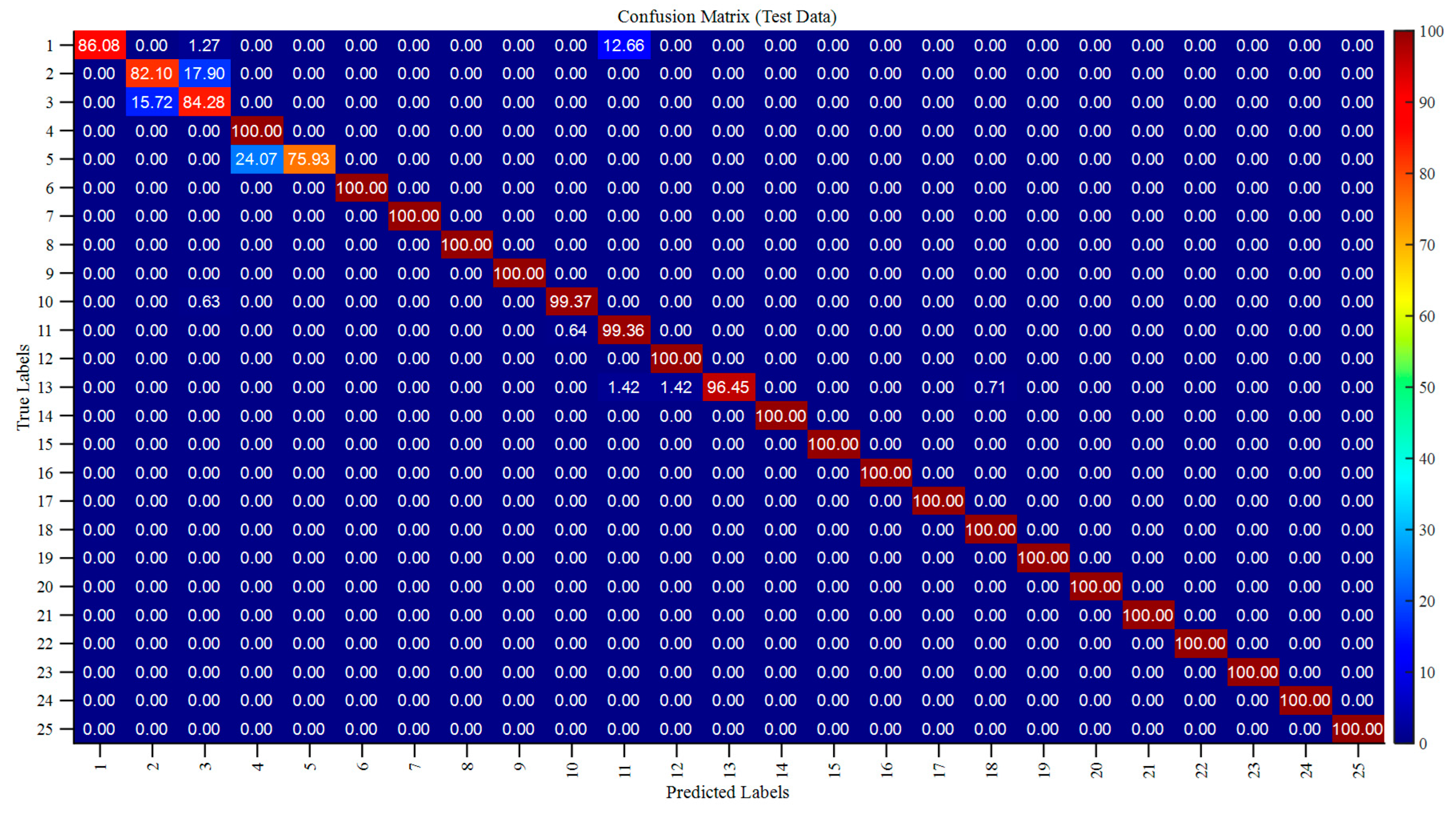
Figure 8 illustrates the confusion matrix for the PSO-SVM model. The experimental results show that the recognition rate of defects in Categories 01–03 is more than 82.1%. Among them, the outer-sheath damage defect causes the fault sheath loop current at the end of the sheath to differ from the simulation results. As the defect location increases in distance from the starting point, the phase angle and amplitude difference of the three-phase sheath voltage initially increase and then decrease. This different feature is significant. For defects of Types 16–24, the recognition rate reaches 100%.

In this paper, in addition to the PSO-SVM classifier, several other classification algorithms are used to identify the states in the cable grounding system, namely SVM, CNN (Convolutional Neural Network), and BP (the feedforward neural network). Due to the dependence on the gradient-descent algorithm, BP is prone to fall into a partial optimum, especially in the case of complex data distribution. The average recognition rate of the model is only 82.89%. Although CNN has significant advantages in image processing, its limitations are more apparent when handling non-image information, particularly data without spatial correlations. The average recognition accuracy of the CNN model is 93.09%. In contrast, SVM classifiers without parameter optimization showed an average recognition rate of only 61.89% for defects. The SVM classification method (i.e., PSO-SVM) using the particle swarm optimization (PSO) algorithm to adjust the parameters shows higher recognition ability, and its recognition accuracy for various types of defects generally exceeds 75.9%, with the average recognition accuracy reaching 97.05%.

In addition, compared to the other three classification models, the PSO-SVM model performs better in the four evaluation metrics, accuracy, precision, recall, and F1 score [40], as shown in

Table 2. Comparison of classification model performance.

Classifier	Accuracy	Precision	Recall	F1-Score
PSO-SVM	0.9976	0.9724	0.9694	0.9695
SVM	0.9701	0.6617	0.6203	0.6159
CNN	0.9943	0.9345	0.9293	0.9301
BP	0.9863	0.8454	0.8319	0.8266

.

The experiments demonstrate that the performance of the PSO-SVM classification method outperforms the other three classifiers, making it more suitable for recognizing and classifying multiple defect states in the grounding system. Additionally, 20 independent experiments were conducted, and the classification accuracy for each experiment was statistically analyzed. The data are as follows: the average classification accuracy of the model is 96.38% with a standard deviation of 0.26%, indicating that the classification model is stable.

4. Grounding System Defect Location

4.1. Fault Impedance Characteristic Location Method

After identifying the grounding system’s defective states, the 04–15 categories in Table 2 can be localized to a specific location. The remaining three open-circuit defects (01–03 categories) and nine cross-bonded segments of the breakdown in the outer sheath caused by grounding defects (16–24 categories) are difficult to locate. To solve the localization problems of these two types of defects, this section presents a localization method based on fault impedance characteristics.

The first and last terminals of the cable are derived simultaneously towards the defective point, and the remaining part of the line other than the fault point for normal conditions can be used to calculate the voltage and current along the line using the cross-bonded cable distribution parameter model in Section 2.1. Figure 9 shows the structure of the circuit under grounded short and open circuits. In the figure, $R_f$ is the transition resistance, $i_{\mathrm{f}\text{\_}\mathrm{left}}$ and $u_{\mathrm{f}\text{\_}\mathrm{left}}$ are the currents and voltages obtained from the beginning terminal calculated to the defect point before the defect, $i_{\mathrm{f}\text{\_}\mathrm{right}}$ and $u_{\mathrm{f}\text{\_}\mathrm{right}}$ are the currents and voltages obtained from the ending terminal calculated to the defect point after the defect, and $i_{\mathrm{f}}$ and $u_{\mathrm{f}}$ are the current and voltage to ground at the transition resistance of the defective outer sheath.

According to Section 2.1, the equations for calculating the voltage and current of the left and right sheathing in the left and right sheaths at the cross-bonded defects are:

$$\begin{array}{l}({\mathrm{u}}_{\mathrm{f}\text{\_}\mathrm{left}},i_{\mathrm{f}\text{\_}\mathrm{left}})=f(u_{\mathrm{ABC}}^{\mathrm{M}},i_{\mathrm{ABC}}^{\mathrm{M}},l_f)\\ ({\mathrm{u}}_{\mathrm{f}\text{\_}\mathrm{left}},i_{\mathrm{f}\text{\_}\mathrm{left}})=f(u_{\mathrm{ABC}}^{\mathrm{N}},i_{\mathrm{ABC}}^{\mathrm{N}},l-l_f)\end{array}$$

(16)

4.1.1. Locating Grounding Defects for Breakdown in the Outer Sheath

Identifying the outer-sheath breakdown defect in Section 3 allows the defect to be localized to a segment of the cross-bonded cable, where only the length of the defect from the beginning of the segment needs to be measured.

This is obtained from circuit theory:

$$\begin{array}{l}{i}_{\mathrm{f}\text{\_}\mathrm{left}}-i_{\mathrm{f}\text{\_}\mathrm{right}}=i_f,u_{\mathrm{f}\text{\_}\mathrm{left}}=u_{\mathrm{f}\text{\_}\mathrm{right}}=u_f\\ \gamma =\angle u_{\mathrm{f}}-\angle i_{\mathrm{f}}\end{array}$$

(17)

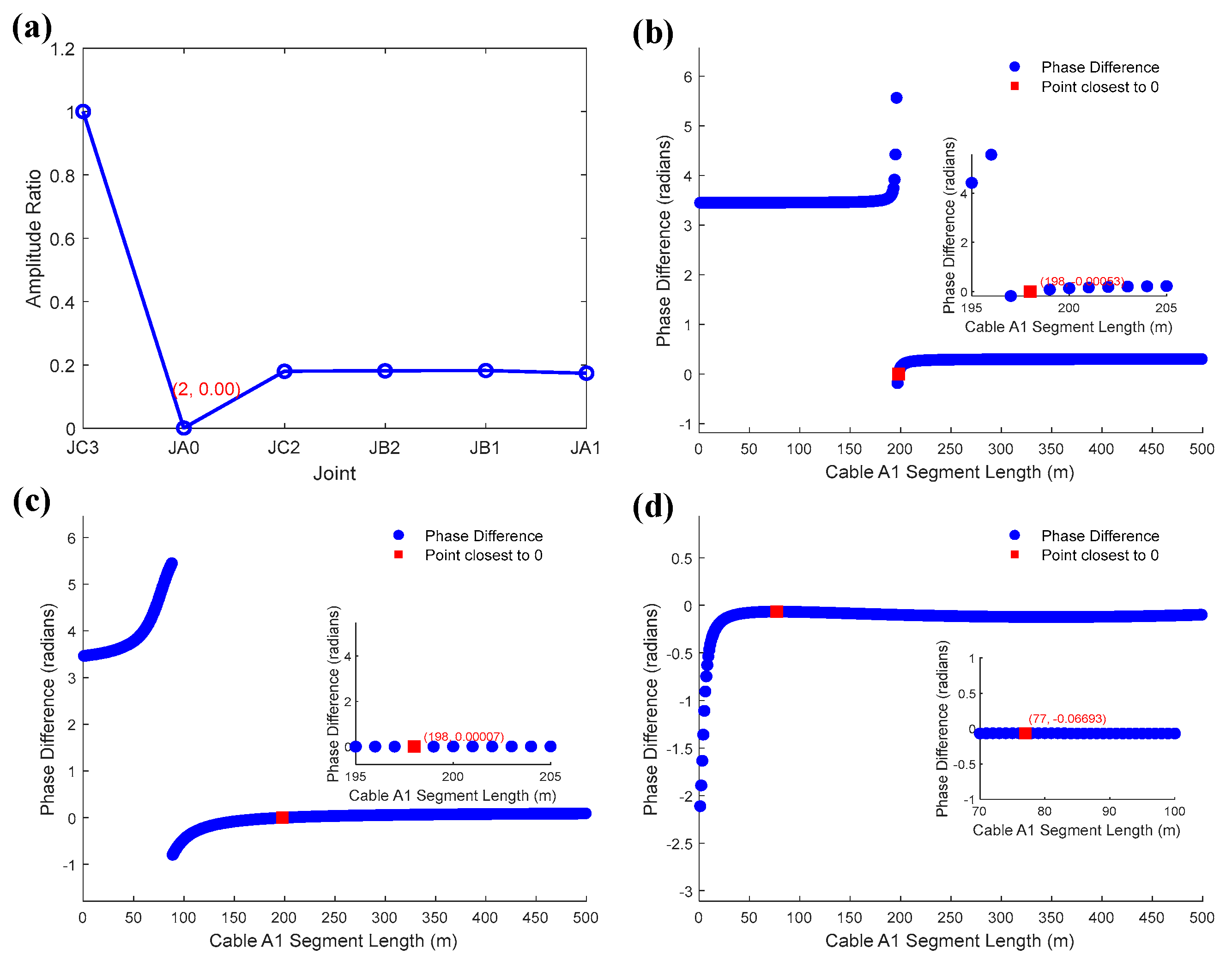
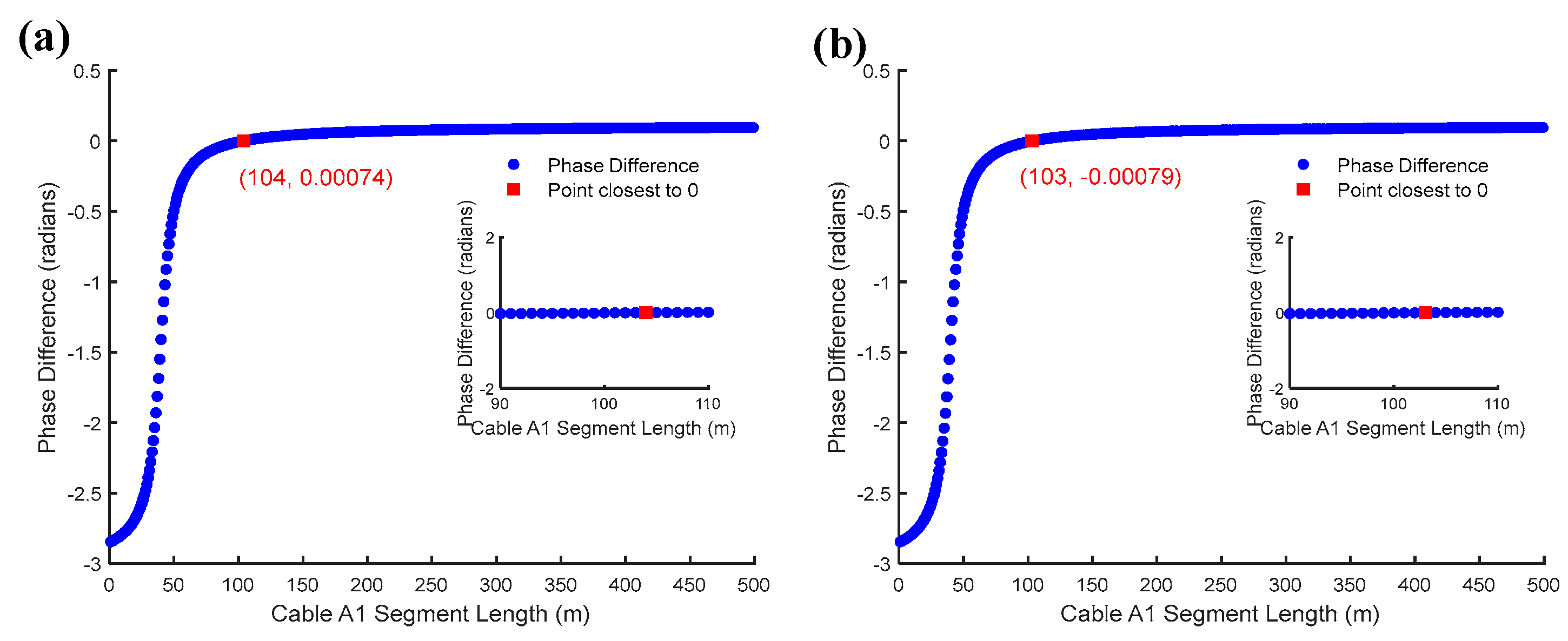
Since the transition resistor is purely resistive, the phase angle difference $\gamma$ between the voltage and current at the defect is 0. Locating the defect turns into a problem of finding the zero-crossing point of $\gamma$ along the cable line.

4.1.2. Locating Open-Circuit Defects

Identifying open-circuit defects in Section 2 allows the defects to be localized to the six joints of the cross-bonded cables, and here only to specific joints.

This is obtained from circuit theory:

$$\mathrm{\eta }=\left|u_{fo}\right|/\left|i_{fo}\right|$$

(18)

$\left|u_{fo}\right|$ is the magnitude of the open-circuit voltage obtained by deducing from the beginning or ending terminal to the defect, and $\left|i_{fo}\right|$ is the magnitude of the open-circuit current obtained by deducing from the beginning or ending terminal to the defect.

If the open-circuit current $\left|i_{fo}\right|$ is 0, then $1/\mathrm{\eta }$ tends to 0, transforming the defect localization into a problem of finding the zero crossing point of $1/\mathrm{\eta }$ at the cross-bonded joint location.

Through the bisection method or minimization of the absolute-values method, the zero-crossing points of curves are $1/\mathrm{\eta }$ and $\gamma$. The cable length corresponding to the zero-crossing point is the desired defect location.

4.2. Localization Algorithm

This paper establishes an equivalent model for the cable circuit and proposes a defective localization flowchart based on the cable fault impedance characteristics, as shown in Figure 10.

The steps are as follows: (1) First, collect the voltage and current data of the core and sheath at both terminals of the cable, calculate the first terminal electric quantity through the first and third partitions of Equation (4) to obtain six moduli, input the beginning terminal modulus into Equation (1) to obtain the ending terminal modulus, and calculate the ending terminal modulus through the second and fourth partitions of Equation (4) to obtain the ending terminal sheath’s voltage and current phase quantity.

(2) Extract the amplitude and phase angle difference between the calculated and sampled values of the ending terminal sheath voltage and current and obtain a 12-dimensional feature vector after feature processing.

(3) Input the feature vectors into the trained PSO-SVM classification model to identify the defect types. The identified types are 04–15 and 25, which locate the fault location; the identified types are 01–03 and 16–24, which perform the locating fault step 4.

(4) Use Equation (16) to calculate the sheath voltages and currents on the left and right sides of the cross-bonded defect. For defects of Types 01–03, use Equation (18) to calculate the value of $1/\mathrm{\eta }$ along the line; for defects of Types 16–24, use Equation (17) to calculate the value of $\gamma$ along the line.

(5) According to the bisection method or the minimization of the absolute-value method, calculate $1/\mathrm{\eta }$ and $\gamma$ along the cable line over the zero point, with the zero point corresponding to the length of the cable $l_{\mathrm{f}}^{\prime }$, which is the location of the defect.

Judge whether the $1/\mathrm{\eta }$ and $\gamma$ at the calculated defect location $l_{\mathrm{f}}^{\prime }$ satisfy the convergence condition of Equation (19). If so, the final defect location is $l_{\mathrm{f}}^{\prime }$. Otherwise, re-execute Step 3, where λ is the threshold value. This paper obtains 0.1.

$$\begin{array}{l}\left|1/\mathrm{\eta }\right|<\lambda \\ \left|\gamma \right|<\lambda \end{array}$$

(19)

4.3. Defect Location Example Analysis

In actual working conditions, the phase angle difference between the voltage and current of the sheath of a high-voltage cable is affected by the transition resistance, the time-invariant factors (three small segments of unequal length), and the time-varying factors (core current, core voltage, and sheath grounding impedance).

An ATP simulation platform with the same cable type and structure as Section 3 is built. Since grounding system defects usually manifest as persistent electrical anomalies, a Fourier algorithm is used to extract the magnitude and phase angle of the steady-state phase at the time of the defect. The following equation expresses the localization error:

$$\mathsf{\theta }=\left|{\displaystyle \frac{{l\prime }_{\mathrm{f}}-l_{\mathrm{f}}}{l}}\right|\times 100\%$$

(20)

${l\prime }_{\mathrm{f}}$ is the distance of the measured defects from the beginning terminal of the cable, $l_{\mathrm{f}}$ is the distance of the set defects from the beginning terminal, and $l$ is the length of the segment of the cable line, taking the defects of sheath breakdown at segment A1 and the defects of open joints at JA0 as examples to validate the defect localization method proposed in Section 4.2.

4.3.1. Analysis of the Effect of Transition Resistance on Defect Localization

After quantitative analysis of the three factors on the defect location, this section controls the voltage root-mean-square (RMS) value of 220 kV (the following core voltage and current are RMS values) and the core current value for the setting of 1497 A, and each small segment is cross-bonded at a length of 500 m, while the beginning and ending terminal grounding resistance are 1 Ω. The transition resistance value is 0.01–100 Ω. Set the A1 segment distance from the beginning terminal of the defect distance of 100 m or 200 m. The above two types of defects are obtained by Section 4.2 to obtain the location results, as demonstrated in Figure 11.

To compare the accuracy of the localization method in this paper with other localization methods, the transition resistance is fixed at 100 Ω, and the distance of the defect point from the beginning terminal of the cable is changed while other conditions remain unchanged. The other methods are localization methods using the aggregate Π model. Method 1 is the method of reference [34], and method 2 is the method proposed in this paper. The comparison accuracy is shown in

Table 3. Position accuracy.

Defect Location	Defect Distance from Beginning Terminal	Method I. Traditional Methods	Method II Methodology of This Paper
Segment A1	100 m	68.6%	95.4%
	200 m	68.4%	99.6%
Segment B2	700 m	68.9%	99.8%
	800 m	67.2%	99.6%
Segment C3	1200 m	69.7%	99.2%
	1300 m	67.9%	94.2%

.

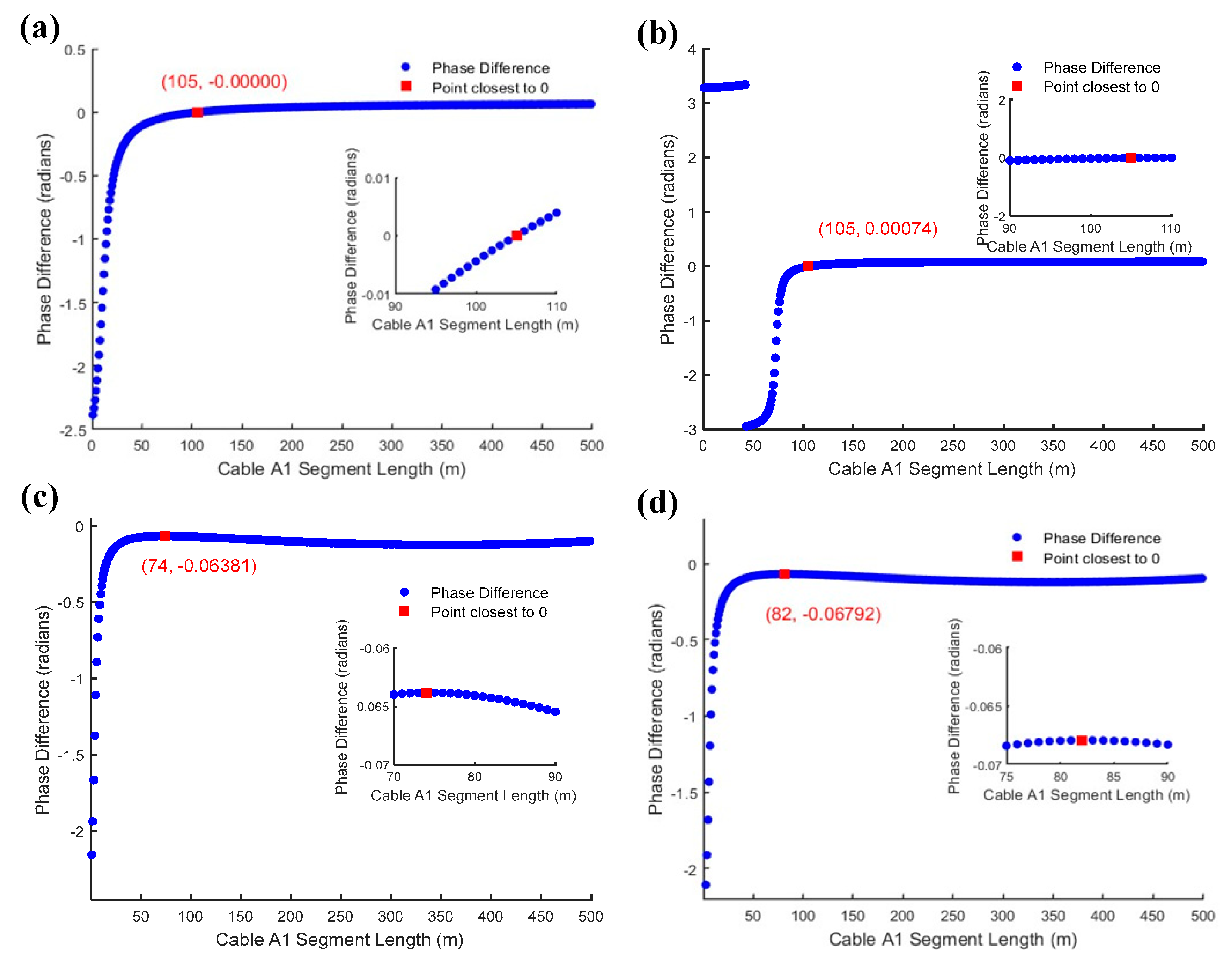
From Figure 11a, it can be seen that the method of this paper can be used to locate the open-circuit defective joint disconnections more accurately, with higher positioning accuracy. According to the analysis of Figure 11b,c, with the increase of the transition resistance value, the defect positioning accuracy decreases. When the defect location is located at 100 m or 200 m of the A1 segment, the positioning accuracy remains above 95.4% when the transition resistance value is small or large; when the transition resistance is 100 Ω, the positioning accuracy is between 99.8% and 91.4%. Overall, the proposed method in this paper significantly improves the localization accuracy compared to the traditional method at larger transition resistor resistance values.

4.3.2. Analysis of the Effect of Time-Varying Factors on Defect Localization

Under the actual working conditions, the core voltage, current, and sheath grounding resistance show fluctuation. In this section, the control variable method is used to investigate the effects of the three factors on defect localization.

First, the core voltage and grounding impedance are controlled as constants: The core voltage is set to 220 kV, the grounding impedance at both terminals of the cable is taken to be 1 Ω, the transition resistor resistance is set to 100 Ω, and the core currents are selected to be 751 A and 2889 A, respectively.

Figure 12 shows that the inductive component of the sheath current increases as the core current increases. The inductive current causes additional voltage distribution in the sheath, changing the voltage and current at the defective point, affecting the measurement results of the defective location and reducing the positioning accuracy. After the amplitude of the core current increases by 284%, the localization accuracy decreases by 0.6%.

Then, the core current and core voltage are controlled to be constant; the core current magnitude is 1497 A, the core voltage is set to 220 kV, and the transition resistor resistance magnitude is 1 Ω. The sheath grounding impedance is set to be 0.1 and 5 Ω.

There is no change in the positioning accuracy of the measured grounding resistance when the transition resistance is 1 Ω. Now, the transition resistance is increased to 100 Ω and the results are shown in Figure 13. The positioning accuracy increases with the increase of grounding resistance. Under low grounding resistance, the sheath current is more likely to be shunted at the cross-bonded grounding point, resulting in a phase shift of the signal at the fault, which reduces the positioning accuracy. In the case of low-transition resistance, the sheath current is more uniformly distributed, and the change in the phase angle difference of the signal is smaller. Under high-transition resistance, the obstruction of the fault point to the sheath current is enhanced, the sensitivity of the signal affected by the grounding impedance increases, and the positioning accuracy decreases by 0.6% after the grounding resistance impedance is reduced by 98%.

Finally, the control core current and grounding impedance are constants, and the core current is set to 1497 A, the sheath grounding impedance is 1 Ω, and the transition impedance is 100 Ω. According to GB/T 12325, the amplitude of working voltage fluctuates no more than ±10%, and the core voltage of 198 kV and 242 kV is taken. The simulation results are shown in Figure 14. The results show that the accuracy of defect localization under working voltage fluctuation is within 99%, and the influence of working voltage fluctuation on localization is very small.

4.3.3. Analysis of the Effect of Time-Invariant Factors on Defect Localization

It is difficult to consistently lengthen the three sections of cross-bonded cables in the actual lines, which will affect the sheath-induced voltage balance relationship and then the phase difference of the sheath current.

To study the impact of cross-bonded cable three-segment lengths on the phase difference of the sheath current, one, two, and three segments were set up with a difference of 100 m [300,400,500] and 200 m [200,400,600]. The defect is located in the A1 segment from the beginning terminal at 100 m. The core voltage was set at 220 kV, the core current was 1497 A, the sheath grounding impedance was 1 Ω, and the transition impedance was 1 Ω.

The results are shown in Figure 15. The unequal length of small segments affects the method of defect localization. However, the effect is insignificant when the difference in the spacing of small segments is 100 m, which is consistent with the localization accuracy of the equal length of small segments in Section 4.3.1. The accuracy decreases by 2.93% when the difference in the length of small segments is 200 m, and the degree of unequal length of small segments must be considered in practice.

5. Conclusions

The main proposal of this paper is a defect identification method for the cable grounding system based on the distribution parameter model, sheath electrical quantity characteristics, and PSO-SVM. For the defects of the sheath loop open circuit and outer-sheath breakdown defects that the classifier cannot localize, the defect localization method of fault impedance characteristics is proposed, and the validity of the method is verified by simulation with high-ranking accuracy.

(1)

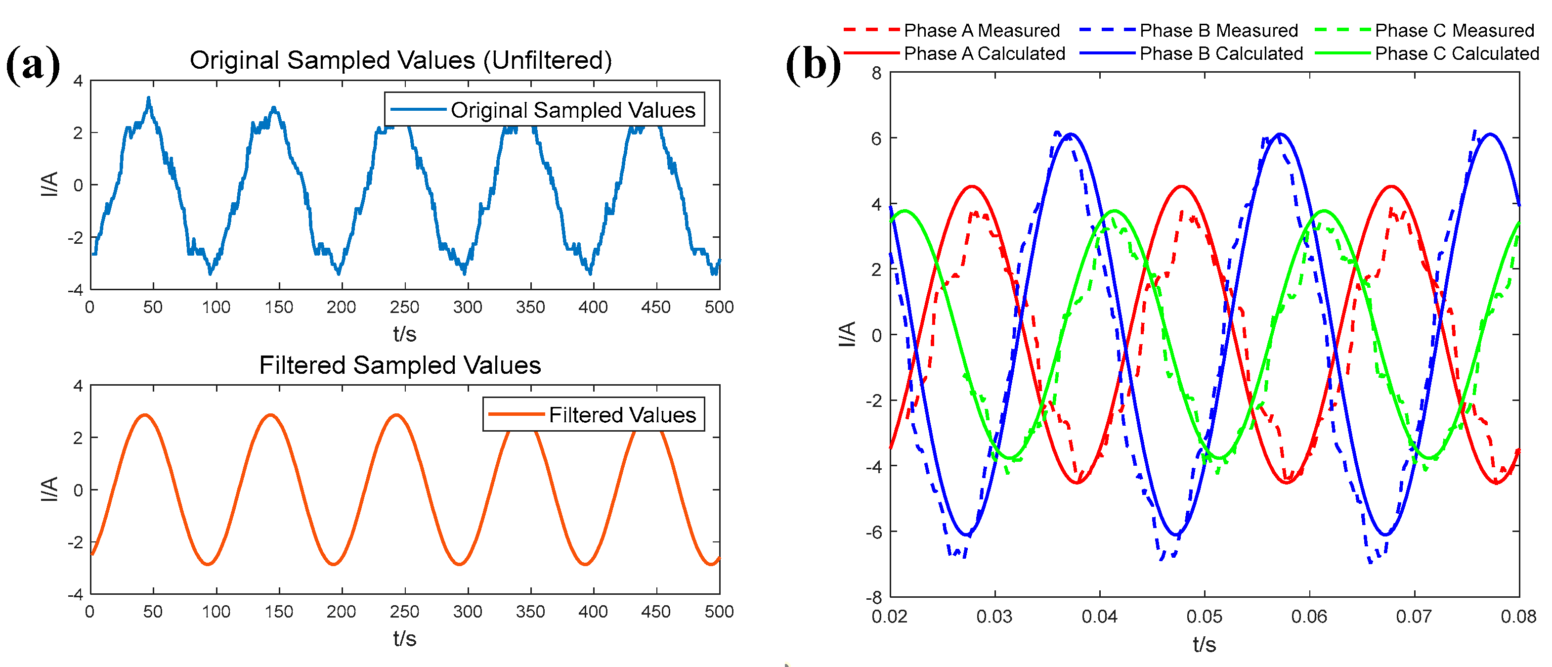
The distributed parameter model proposed in this paper considers the coupling structure between the core and sheath, as well as the higher-order terms of infinitesimal segments. Both simulation results and actual data validate the accuracy of the model in simulating the electrical quantities of the core and sheath in cross-bonded cables.

(2)

Using the difference between the ending terminal sampling and calculation in the defective state of the cable grounding system, and considering the phase angle and amplitude characteristics of the sheath voltage and current, the accuracy rate of 25 cross-interconnection cable grounding system state identifications based on the PSO-SVM classification model reaches more than 97%.

(3)

Based on the characteristics of sheath current and voltage under the open-circuit defect of the sheath circuit and the outer-sheath breakdown defect, the localization problem is transformed into a problem of solving the two curves over the zero point. The validation of the algorithms shows that the method can accurately locate the faulty joint position in the case of JA0 joint open-circuit defects. In the case of outer-sheath breakdown defects in the A1 segment, the localization accuracy is no less than 99.6% when the transition resistance is low (0.01–1 Ω). When the transition resistance is high (100 Ω), the localization accuracy is significantly improved compared with the other methods, which shows the method’s advantage in high-resistance fault conditions.

(4)

The effects of core voltage, core current, grounding resistance, transition resistance, and inconsistent length of cross-bonded cable segments on defect localization are studied and analyzed. The simulation results show that the working voltage fluctuation has less influence on the localization accuracy. The increase of the core current causes the inductive component of the sheath current to be enhanced, and the localization accuracy slightly decreases. When the transition resistance is 100 Ω, the localization accuracy is enhanced with the increase of grounding impedance, which shows high sensitivity. A cross-bonded cable segment length difference of 100 m has less impact on the positioning accuracy, consistent with the equal length, while with the difference of 200 m, the positioning accuracy decreased by 2.93%. In practical application, paying attention to the influence of grounding resistance and segment length inconsistency on positioning accuracy is necessary to improve the method’s reliability.

The dataset used in this paper covers 25 common state types in the grounding system, and the sample distribution is balanced and representative, which can comprehensively reflect the diversity of typical defect identification in practical applications. Therefore, the PSO-SVM model achieves a high recognition rate on this dataset, proving its good classification performance under the current data.

In this study, only real-world tests have been conducted for the validation of the cable distribution parameter model, and real-world tests have not yet been conducted for grounding system state identification and defect localization. Future work will introduce real-world testing to increase real-world defect identification data and verify the general applicability of the proposed method for defect identification and localization.