Abstract
The rise of direct current (DC) distribution networks, driven by distributed energy storage and large-scale photovoltaic integration, has significantly altered distribution network configurations. In DC networks, short-circuit faults cause a sharp drop in voltage and a rapid increase in current, negatively impacting system stability. To solve this problem, we used an improved red fox optimization (IRFO) algorithm to calculate the distance to failure of the protection device. The algorithm shows higher convergence and accuracy compared to conventional methods. The isolated forest algorithm rejects anomalous data, while an adjustable feedback factor and genetic crossover operator further improve performance. Adaptive interpolation is employed to address low sampling frequency issues, enhancing fault localization precision. Simulations performed in Simulink show that the method is highly resistant to interference with minimal localization error. It is also resistant to changes in system parameters, highlighting its robustness and usefulness in fault localization.
1. Introduction
At present, China’s traditional AC distribution network is still in a dominant position. With the transformation of the global energy structure and the large-scale accessibility of renewable energy, the traditional AC distribution network has significant deficiencies in energy efficiency, equipment complexity, system stability, convenience of new energy access, and fault handling speed, etc. The DC distribution network has become an important development direction of the future smart grid because of its high efficiency, reliability, and flexibility [1]. The DC distribution network has gradually become an important development direction of the future smart grid due to its high efficiency, reliability, flexibility, and other characteristics [1]. Compared with the traditional AC distribution network, the DC distribution network has the following advantages: (1) strong power supply stability; (2) higher flexibility, which is conducive to the accessibility of renewable energy; and (3) better economy. Compared to the AC distribution network, the DC distribution network has a lower degree of technical maturity and lacks unified technical standards and norms, which leads to certain technical risks in practical application [2]. At the same time, the key equipment in DC distribution grids, such as converters and circuit breakers, is currently of a high cost, which increases the construction cost of the system [3]. In addition, DC transmission protection and control strategies are complex. The DC distribution network has a fast-rising fault current, no over-zero point, difficult arc extinguishing, and a complex system structure, which makes the formulation and implementation of protection and control strategies complicated [4]. Due to the small damping of the DC distribution network, the intermittency and randomness of distributed power sources are prone to affect the stable operation of the DC distribution network and increase the difficulty of system regulation and control [5]. Therefore, it is of great research significance to study reliable protection strategies for DC distribution networks containing new energy sources, such as wind turbines, photovoltaic, energy storage, and DC loads, to improve the ability of accurate fault localization in DC distribution networks and to guarantee the reliability of the power supply in distribution networks [6].
At present, the methods employed for locating power system faults can be categorized into three distinct classes: the traveling wave method, the applied injection signal method, and the fault analysis method [7]. The traveling wave method, as previously outlined, is predicated on the analysis of propagation time and waveform characteristics between the fault point and the traveling wave measurement point. This method has been shown to exhibit both high accuracy and efficiency. However, this method is susceptible to interference from external factors and has high requirements on the sampling frequency of the equipment as well as the operator’s skills. In high-resistance grounding systems, the accuracy of fault location will be significantly reduced. One method of signal injection involves the injection of specific signals and the subsequent analysis of the detection signal to determine the fault location [8]. This method exhibits higher fault line accuracy, but it is susceptible to external environmental interference. Additionally, its resistance to transition resistance is poor. Another method of fault analysis involves the use of fault conditions to measure the voltage and current of components [9]. This method is based on the structure of the distribution network and the operating characteristics of the list of differential equations of the fault distance. It is simple, easy to implement, and practical. As outlined in [10], a DC distribution network fault location method based on the differential initial value of current is proposed. This method is applicable to lines equipped with current-limiting reactors. It involves analyzing the voltage drop of the current-limiting reactors at the outlet of the VSCs and utilizing the rate of change in the current for fault location. However, this method has more stringent requirements for data synchronization. Synchronizers must be installed at both ends of the line, resulting in higher installation costs. As posited in the literature [11], the equation is solved through the analysis of the voltage characteristics of the current-limiting reactor to determine the location of the fault point, which possesses both fast and accurate localization capabilities. However, this method necessitates a high sampling frequency of the system. In the event that the sampling frequency is inadequate, the error of fault localization will increase significantly. Nevertheless, the literature does not provide a solution to this problem. As posited in the literature [12], a methodology for fault localization in double-ended DC distribution systems is proposed. This methodology involves the measurement of fault voltages at both ends, the construction of voltage matrix equations, and the solution of fault line resistance parameters. The method has been shown to achieve high localization accuracy; however, in a multi-terminal ring network, the calculation process is more complicated compared to a double-terminal distribution network. It is imperative to consider the current injected into the fault point by other converter stations, excluding neighboring converter stations, to ensure the accuracy of the method. Conventional fault localization methodologies have been observed to generate substantial localization errors in multi-terminal distribution networks.
In recent decades, artificial intelligence algorithms have been widely used in various fields by virtue of their great advantages. One study [13] proposed the design of a trusted hybrid encryption algorithm using DNA layers and the AES by utilizing the characteristics of DNA layers and the AES combined with an AI algorithm, which was able to show that IoT (Internet of Things) signals could be enhanced with encrypted data. Another study [14] proposed the utilization of a Genetic Algorithm for parameter identification to realize the accurate localization method of DC distribution line faults, which was resistant to transition resistance and highly robust. In 2023, Hardi M. Mohammed proposed a new stochastic optimization algorithm, red fox optimization (RFO), which seeks the optimal solution to a problem by simulating the hunting behavior of red foxes and has the advantages of a fast convergence speed and high accuracy. A previous work [15] applied the red fox algorithm to the ship spare parts prediction model, and the simulation results proved that the red fox algorithm has a stronger ability to find the optimal solution and that the comprehensive performance is better. Another work [16] studied the red fox optimization algorithm on the basis of the introduction of a chaos algorithm to improve global search ability, and its application to the particle filter lithium battery remaining life prediction research proved that the red fox algorithm has better convergence and robustness. The literature [17] on the previous ship spare parts demand prediction accuracy is not extensive and cannot address the actual problem of the comprehensive protection of ships. The red fox algorithm has been combined with the support vector regression (SVR) algorithm to further improve the optimization accuracy of the red fox optimization (RFO) algorithm and integrate the elite reverse learning strategy. However, the abovementioned methods have not been applied in distribution network fault localization.
In addressing these issues, this paper proposes a multifaceted approach. It involves the collection of voltage data at both ends of the line, the consideration of currents injected at the fault point by converter stations other than neighboring stations, the modeling of inter-pole faults and single-phase short-circuit faults of the DC system, the formulation of double-ended voltage equations that eliminate transfer impedance, and the construction of a matching function. The present study investigates the impact of low sampling frequency, single-sampling-point anomalies, transient impedance, and other factors on the fault localization accuracy of a DC distribution system. This investigation utilizes a simulation approach to examine the system’s performance under these conditions [18]. The simulation results demonstrate that the multi-terminal DC distribution fault localization method based on the modified red fox algorithm can achieve accurate DC distribution fault localization.
In the context of DC distribution networks, ring, loop, and two-way feeder topologies are prevalent. The chain-structured configuration is characterized by its simplicity in wiring and relatively low construction cost. However, it is associated with suboptimal reliability, poor voltage stability, and limited scalability. The two-terminal feeder exhibits high reliability and a relatively straightforward line structure, making it well suited for use in regional power plants. Nonetheless, it faces challenges in meeting the demand of new loads and possesses limited scalability. The toroidal feeder is distinguished by its high reliability, high power quality, and flexible scheduling.
In this paper, the multi-terminal ring network structure is employed, and its topology is illustrated in Figure 1.
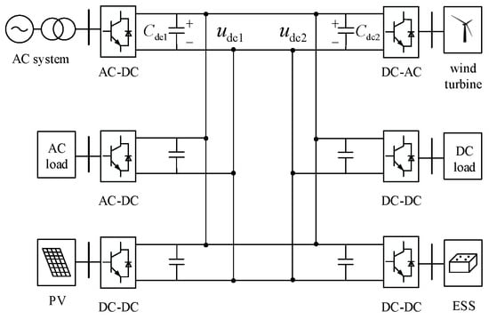
Figure 1.
Topology structure of six-terminal DC distribution network.
2. Fault Characteristics of DC Distribution Network
Short-circuit faults represent the most prevalent type of fault in DC distribution networks. In such cases, the fault current peaks rapidly over the course of a few milliseconds, precipitating a precipitous decline in line voltage and engendering a grave threat to the integrity of the power system. Consequently, the prompt and precise identification of the fault location is paramount. The progression of a short-circuit fault within a DC line can be categorized into three distinct stages [19]: the capacitor discharge stage, the diode renewal stage, and the steady-state stage. In practical engineering applications, the timely removal of faults in the capacitive discharge stage is instrumental in facilitating the rapid restoration of power supply to the system. Consequently, the primary focus of this paper is the analysis of the capacitive discharge stage [20].
2.1. Fault Characteristics of Inter-Electrode Short Circuit
In the event of a short-circuit fault between poles, the current in the line undergoes a rapid increase. To ensure its own protection, the IGBT blocks the drive signals of all bridge arms. At the onset of the fault, capacitive discharges at both ends of the converter generate capacitive currents, leading to the injection of short-circuit currents from the AC side to the DC side. The interplay of these currents culminates in the formation of a fault current, wherein the influence of the capacitive discharge current assumes a dominant role [21].
A schematic diagram of the capacitive discharge stage fault of a DC line with an inter-pole short circuit is shown in Figure 2.
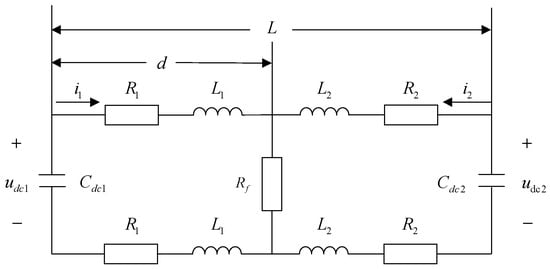
Figure 2.
Equivalent circuit diagram of inter-polar short-circuit fault capacitance discharge stage.
In Figure 2, , , , and are, respectively, the resistance and inductance from the fault point to the VSC at both ends of the transmission line. and are the capacitance to the ground. is the transition resistance; and are the voltages at both ends of the capacitor.
The voltage and current waveforms after the inter-electrode short-circuit fault occurs at both ends of the line are shown in Figure 3 and Figure 4.
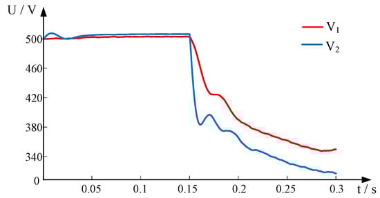
Figure 3.
Voltage waveform of inter-pole short-circuit fault.
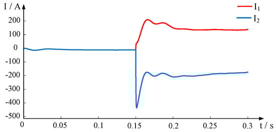
Figure 4.
Current waveform of inter-pole short-circuit fault.
Derivation of the loop equations is predicated on Kirchhoff’s voltage law, which enables the subsequent calculation of the voltage and current relationship from the line outlet to the point of fault:
Similarly,
Equations (1) and (2) both contain transition resistance , and by combining the above two formulas to eliminate the influence of the transition , the following can be obtained:
In Equation (3), , and are, respectively, expressed by the resistance and inductance parameters per unit length:
where is the unit length resistance, is the unit length inductance, is the length between the fault point and the first end of the line, and is the total length of the DC transmission line.
By substituting Equation (4) into Equation (3), the location distance of the short-circuit fault between electrodes is
2.2. Single Pole Ground Short Circuit Fault Characteristic Analysis
Unipolar grounding faults are less hazardous than inter-pole short circuits; however, they account for over 70% of DC line faults. Therefore, the localization study of unipolar short-circuit faults is of great significance [22].
The equivalent circuit diagram of the capacitive discharge stage of a unipolar grounding fault occurring in a DC transmission line is shown in Figure 5.
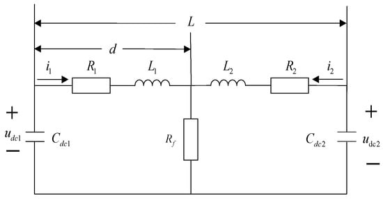
Figure 5.
Equivalent circuit diagram of unipolar short-circuit fault capacitance discharge stage.
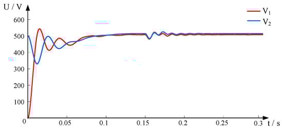
Figure 6.
Single-pole ground fault voltage waveform.
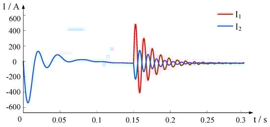
Figure 7.
Single-pole ground fault current waveform.
Derivation of the loop equations is predicated on Kirchhoff’s voltage law, which enables the subsequent calculation of the voltage and current relationship from the line outlet to the point of fault:
Similarly, the following applies for the wind turbine side:
Equations (6) and (7) both contain transition resistance , and by combining the above two formulas to eliminate the influence of the transition, the following can be obtained:
By substituting Equation (4) into Equation (8), the single-pole short-circuit fault location distance is
2.3. Calculation of Microcomponents
On the assumption that the capacitor voltage sampling at both ends of the AC side and the fan side is completely synchronized, the differential method is used to calculate the voltage change rate for the voltage micro-components in Equations (3) and (6). And the sampling time is 10 microseconds. The voltage micro-component in Equations (3) and (6) can be expressed as follows:
where represents the sampling point; , and represent the voltage value at three consecutive sampling points; represents the time interval between two consecutive sampling points.
3. Red Fox Optimization Algorithm
The resolution of Equations (5) and (9) solely necessitates the voltage data at both extremities of the DC line. Nevertheless, relying on a solitary set of voltage data for fault localization engenders highly unstable localization outcomes due to the presence of measurement errors. To circumvent this challenge, the RFO (red fox optimization algorithm) [23] is employed to ensure precise fault localization, leveraging a comprehensive set of 500 voltage data points following the occurrence of a short circuit.
The RFO algorithm is a computational model that simulates the hunting behavior of a red fox. This algorithm has been shown to have the advantages of fast convergence and high accuracy. The RFO algorithm consists of three main stages [24].
RFO consists of the following three stages [25]:
- Initialization:
The population size must be set, and the initial position and state parameters must be randomly generated.
- 2.
- Hunting behavior simulation:
The algorithm simulates the red fox by updating its position. During the hunting behavior simulation, the probability of the red fox hunting in a positive direction is 82%, and the probability of hunting in the opposite direction is 18%. This strategy compels the red fox to deviate from the local optimal solution and pursue a more optimal global solution.
- 3.
- Update solution set:
The set of candidate solutions is updated based on the results of the hunting simulation. The solutions with higher fitness are retained, while the solutions with lower fitness are eliminated. As the number of iterations increases, the candidate solution set gradually converges to the optimal solution.
4. Application of Improved Red Fox Optimization in Fault Location
The conventional RFO algorithm is susceptible to issues such as elevated parameter sensitivity and proclivity for local optimization. To address these limitations, this paper puts forward an IRFO algorithm for the localization of faults in distribution networks. The proposed methodology involves the elimination of abnormally sampled data through the integration of the isolated forest algorithm. Additionally, it mitigates the impact of low sampling frequency on fault localization by employing the cubic spline interpolation method. Furthermore, it enhances search speed and facilitates the escape from local optimal solutions through the combination of the adaptive feedback factor and the genetic crossover operator strategy. The efficacy of the proposed approach is substantiated by simulation results, which demonstrate the IRFO’s superior performance in fault localization within distribution networks.
4.1. Isolated Forest Algorithm
The isolated forest algorithm is a rapid anomaly detection method [26] that boasts linear time complexity and high accuracy. It also demonstrates greater robustness than traditional machine learning clustering algorithms.
In scenarios where the number of abnormal samples is minimal and geographically distinct from other normal samples, these abnormal samples can typically be isolated after a limited number of cuts. In contrast, normal samples necessitate a greater number of cuts to achieve the same outcome. By repeatedly executing this process, multiple isolated trees are constructed, eventually forming an isolated forest. Subsequent to this, each sample point is substituted into the constructed forest, and its anomaly score is calculated according to the following equation:
where is the height of sample , and is the average length of path after standardization. If the score is close to 1, it is an abnormal data point; if it is much less than 0.5, it is a normal data point; and if it is about 0.5, it indicates that there are no abnormal constant points.
4.2. Adaptive Feedback Factor Is Introduced
In the event of a short-circuit fault within the DC distribution network of a power system, there is a precipitous decline in short-circuit voltage concomitant with a rapid escalation in short-circuit current. In scenarios where the sampling frequency of the system is inadequate, the step change in voltage and current following the short-circuit is not accurately captured. This, in turn, compromises the precision of fault localization.
Cubic spline interpolation is a method of fitting a smooth and continuous function curve through a large number of given data points with low multinomial approximation [27]. Newton interpolation and cubic spline interpolation are both commonly used interpolation methods. However, the former requires a significant amount of computational effort, and the error increases when high-degree polynomial interpolation is performed [28]. In comparison, cubic spline interpolation possesses notable advantages, including its small computational volume, high stability, and smooth interpolation curve. Consequently, it is particularly well suited for rapid fault localization in distribution networks.
4.3. Introduce Adaptive Feedback Factor
The feedback factor is indicative of the relationship between the population of red foxes and the density of their prey. The performance of the algorithm is influenced by the value of the feedback factor, which can be too small or too large. To address this challenge, this paper proposes an adaptive adjustment strategy for the feedback factor. Initially, when the prey density is minimal, the value of the feedback factor is decreased to impede the algorithm from attaining a local optimal solution. Consequently, the value of the feedback factor accelerates decline, thereby enhancing the global search capability of the algorithm. Conversely, as the iteration progresses towards its conclusion, the prey density escalates. Consequently, the feedback factor value stabilizes, thereby facilitating the identification of the optimal solution that corresponds to the highest prey density.
The improved mathematical model of the adjustable feedback factor is
where is the maximum number of iterations, is the current number of iterations, and is the regulatory factor. A comparison of the adaptive adjustable feedback factors when the linear feedback factor and the adjustment parameter k are taken as 1, 4 and 7, respectively, is shown in Figure 8.
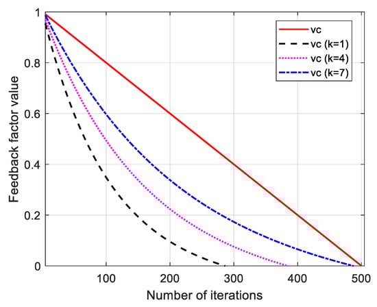
Figure 8.
Feedback factor graph.
As can be seen from Figure 8, the descending speed of the improved feedback factor curve increases with the increase in the adjustment factor k. Therefore, the value of k should not be too large or too small. Therefore, the selection of the k value should not be too large or too small, as too large a k value may lead to the convergence of the algorithm too quickly in its early stage, causing the algorithm’s development ability to weaken and fall into the local minima; conversely, when the k value is too small, it cannot reflect the advantage of the feedback factor in the balance of the algorithm’s search ability, thus slowing the algorithm’s convergence speed down. In order to balance the search ability of the algorithm, the authors of this paper conducted a large number of experimental analyses and finally selected k = 4 as the most appropriate.
4.4. An Adaptive Genetic Crossover Operator Is Introduced
In order to accelerate the convergence speed, this paper proposes the implementation of an adaptive genetic crossover operator. This operator enables a certain possibility for the current sample to genetically cross over with the optimal sample. The mathematical model is delineated in Equation (13) [29]:
where is the current sample location of the red fox, is the optimal sample location of the current population of the red fox, and and are two new sample locations generated after genetic crossover.
The crossover operator realizes continuous updating of the population, while the size of L determines the updating rate of individuals in the population, and if its value is too large, it will destroy the good genetic pattern. Too small a value will lead to slow search speed of the algorithm and difficulty evolving the population. In the pre-evolutionary stage, the value of L should be increased in order to expand the overall search range and accelerate the population renewal rate. In the late stage of evolution, the overall solution set of the population tends to be stable, and in order to continue to preserve the good gene structure, L should be appropriately lowered. In addition, the crossover algorithm can change or even destroy the gene structure; for the poorly adapted individuals, more participation in crossover operations can promote continuous optimization, so they should be given a higher L. Correspondingly, for individuals with higher adaptability, in order to prevent the destruction of the gene structure, the probability of crossover operations should be smaller. The higher the fitness of an individual, the lower the probability of crossover operations should be to prevent the destruction of the gene structure. Based on the above considerations, the sample crossover probabilities are shown in Equations (14) and (15):
where is the maximum number of iterations, is the current number of iterations, = 0.6, the value is related to the number of iterations, is the current sample fitness, is the average fitness of the population, and is the maximum fitness of the sample.
4.5. Construct IRFO Fitness Function
The fault location fitness function based on the IRFO algorithm is
where is the total number of sampling points, selects the calculated value on the left side of Equation (5) or Equation (9) according to different short-circuit types, and is the identification value.
For , the theoretical value is 0; the smaller the fitness function, the better the individual and the stronger the fitness.
4.6. IRFO Fault Location Workflow
- Obtain the voltage data at both ends of the faulty line.
- Check the data for anomalies, and if there are anomalies, use the isolated forest algorithm to eliminate them.
- Judge whether the data satisfy the conditions, if not, carry out adaptive interpolation processing.
- Initialize the population and set relevant parameters.
- Construct the IRFO fitness function s and evaluate the fitness of each sample.
- Check whether the genetic crossover probability is satisfied, and if so, perform the genetic crossover operation.
- Execute jump predation and random wandering strategies to update the optimal sample and its fitness.
- Determine whether the termination condition or the maximum number of iterations has been reached and end the iteration if it is satisfied; otherwise, return to Step (6) to continue the cycle.
The IRFO fault localization process is shown in Figure 9:
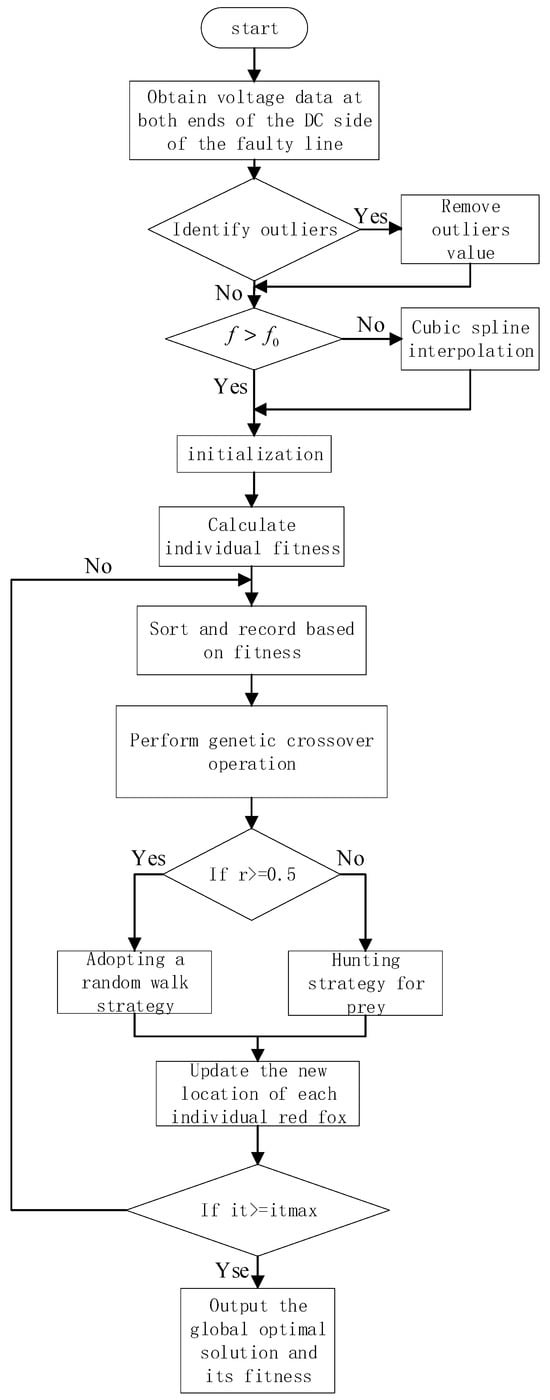
Figure 9.
IRFO fault localization flowchart.
5. Simulation Verification
This paper builds a DC distribution network as a six-terminal ring network as shown in Figure 1. The simulation model diagram is shown in Figure 10.
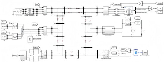
Figure 10.
Simulation model diagram of a six-terminal DC distribution network.
- (1)
- Wind turbine unit: Permanent Magnet Synchronous Generators (PMSGs) are used, which are injected into the DC grid through the VSC. The turbine control adopts Maximum Power Point Tracking (MPPT) to maximize the capture and utilization of wind energy.
- (2)
- DC load unit: DC loads are connected to the DC grid through a DC-DC converter.
- (3)
- AC load unit: AC loads are connected to the grid through a voltage source converter (VSC).
- (4)
- Energy storage and photovoltaic unit: The energy storage unit adopts lead–acid batteries for energy storage and is connected to the DC distribution grid through a boost converter. The photovoltaic unit adopts Maximum Power Point Tracking (MPPT) and is connected to the DC distribution grid through a boost converter.
- (5)
- Large grid-connected unit: It is connected to the DC grid through a voltage-based PWM VSC with direct current control, i.e., current PI control for the inner loop and P-U sag control for the outer loop [30].
The VSC on the AC system side employs a dual closed-loop control strategy, while the VSC on the turbine side functions using a maximum power control mode. The energy storage system plays a pivotal role in maintaining the overall power balance of the system and facilitating islanded operation when required. The PV system is connected to the DC system through a DC-DC converter by the maximum power tracking control mode [31]. Table 1 shows the parameters of the six-terminal DC power distribution system.

Table 1.
Partial parameters of DC distribution network system.
The relevant parameter settings of the IRFO are shown in Table 2. The input data comprise 500 sets of voltage samples from both ends of the line following the occurrence of a short circuit, and the objective function is the IRFO fitness function shown in Equation (16).
Table 2.
Algorithm parameter value.
5.1. Influence of Fault Distance and Transition Resistance on Fault Location
The transition resistance of a short circuit between poles is chiefly determined by the arc resistance. Consequently, the transition resistance between two lines is negligible [32]. In this paper, the maximum transition resistance is set to 5 Ω.
The transition resistance of a single-pole ground fault is more intricate. It is affected by the aging of and damage to the insulation of equipment, environmental factors, and mechanical vibration, among other factors [33]. Therefore, the variation range of the transition resistance is set from 0 to 100 Ω in this paper.
The formula for calculating the fault location error rate is
where represents the error rate of fault location; represents the fault distance; and represents the practical fault distance.
The fault location error rates of the DC distribution network under different transition resistances and different fault distances are shown in Table 3 and Table 4.
Table 3.
Simulation results of inter-polar short-circuit fault.
Table 4.
Simulation results of single-pole short-circuit fault.
As demonstrated in Table 3 and Table 4, the transition resistance exerts a negligible influence on fault localization in DC distribution networks. In the absence of transition resistance, the localization error rates for both interpole and single-pole ground faults are maintained below 0.8%. Even in the presence of transition resistance, the localization error rate is consistently constrained at approximately 1.5%. These findings suggest that the IRFO-based fault localization method exhibits notable resistance to transition resistance, demonstrating its effectiveness and robustness.
The error rates for locating interpole faults and single-pole faults are shown in Figure 11 and Figure 12.
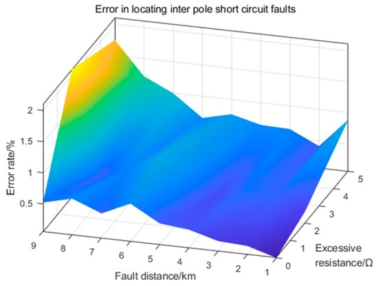
Figure 11.
Error rate of interpole short-circuit fault localization.
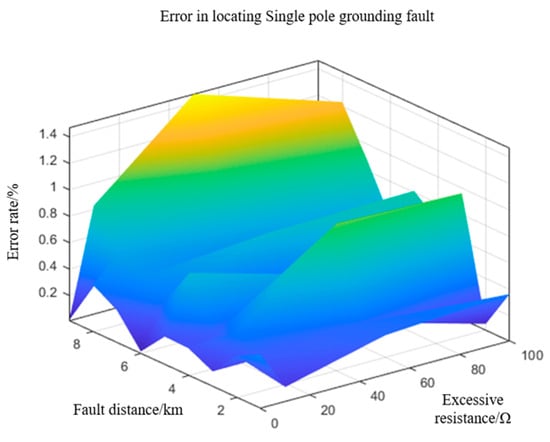
Figure 12.
Error rate of single-pole grounding fault location.
5.2. Effect of Sampling Frequency on Fault Localization
Fault analysis methods have high requirements on sampling frequency: if the sampling frequency is too low, it may lead to the distortion of fault signals [34], which will increase the error rate of fault localization. In practical applications, this will lead to an increase in the workload of line patrol workers. However, enhancing the hardware sampling frequency will bring additional equipment investment costs and put higher requirements on the hardware.
When the sampling frequency is 10 kHz, the fault localization results of the bipolar short-circuit fault DC distribution network are shown in Table 5.
Table 5.
Location results of inter-pole short-circuit faults at a sampling frequency of 10 kHz.
As illustrated in Table 5, when the sampling frequency is low, the fault location error rate exhibits a marked increase, consequently hindering the accuracy of fault location. To address this challenge, this paper proposes the implementation of an IRFO algorithm, which facilitates the adaptive interpolation of the DC distribution network’s pole-to-pole indirect fault voltage within the range of 10 kHz to 100 kHz. The comparative analysis of the fault voltage prior to and following the interpolation process is illustrated in Figure 13.
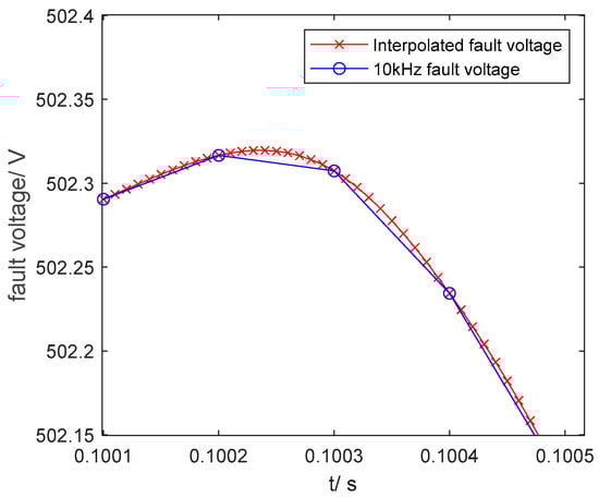
Figure 13.
Fault voltage before and after interpolation.
The voltage data at both ends of the DC line after interpolation are used to locate faults. The fault location results are shown in Table 6.
Table 6.
Location results of inter-pole short-circuit faults at a sampling frequency of 10 kHz.
The comparison of fault location error rates after interpolation is shown in Figure 14.
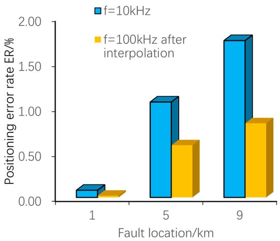
Figure 14.
Comparison of fault localization error rates after interpolation.
From Figure 14, it can be seen that the fault localization error rate undergoes a substantial reduction following adaptive interpolation to 100 kHz. At a distance of 9 km, the localization accuracy of the 0-transition resistance bipolar short-circuit fault is approximately doubled. For a 10 km transmission line, the deviation of the fault localization point from the actual fault point is only 0.0823 km, which effectively reduces the fault localization error of the DC distribution network caused by the low sampling frequency. This helps workers quickly locate the fault point, carry out repairs in a timely manner, and restore the power supply.
In order to verify the accuracy of fault localization of IRFO at different sampling frequencies, simulation experiments were carried out at 10 kHz, 25 kHz, 50 kHz, and 80 kHz. The experimental results are shown in Figure 15.
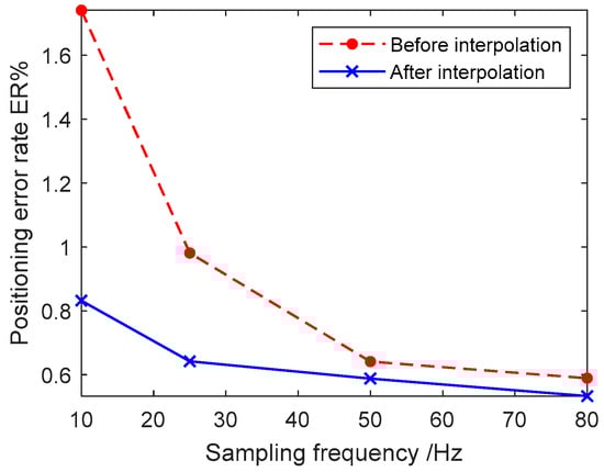
Figure 15.
Error rate of fault localization at different frequencies.
The experimental results demonstrate that IRFO can effectively enhance the accuracy of fault localization when the sampling frequency is low. Furthermore, the error rate of fault localization is consistently maintained below 1% following adaptive interpolation processing.
5.3. Impact of Sampling Data Asynchrony on Fault Localization in Distribution Networks
The experimental results show that IRFO can effectively improve the fault location accuracy when the sampling frequency is low, and the fault location error rate is less than 1% after adaptive interpolation.
In practice, the sampling data at both ends of the transmission line may be out of sync due to communication delays or electromagnetic interference. To model this scenario, this paper misaligns the collected voltage data at both ends by 20 sampling points (i.e., 2 milliseconds) to simulate the data desynchronization condition.
As shown in Figure 16, the fault location error rate for the DC transmission line is consistently within 1% when the sampled data are not synchronized. Regardless of the fault location and fault type, it is within the acceptable error range.
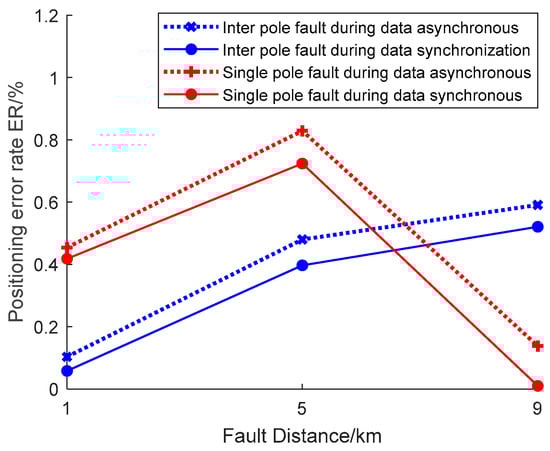
Figure 16.
The impact of asynchronous sampling data on fault localization.
5.4. Impact of Abnormal Sampled Data on Distribution Network Fault Location
In practice, individual sampling data may be deemed abnormal due to transformer failure, environmental factors, and other reasons. To emulate this scenario, this paper designates 5% of the voltage at both ends as abnormal data. The simulation experiment is predicated on the assumption of a 5 km inter-pole short-circuit fault in the DC distribution network, with the fault voltage depicted in Figure 17a. Utilizing the IRFO fault localization algorithm, the abnormal and missing data can be effectively rejected, as demonstrated in Figure 17b. Following the elimination of abnormal data, the fault localization error rate is depicted in Figure 17c.
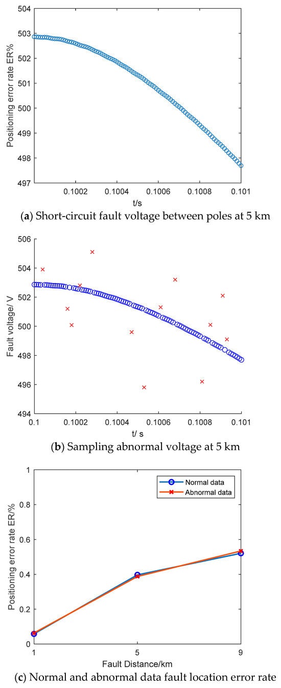
Figure 17.
The impact of sampling anomalies on fault localization errors.
It can be seen from Figure 17 that in the case of abnormal sampled data, IRFO’s fault location is not affected and can still achieve precise positioning in a short time.
5.5. Impact of Running Parameters on Fault Location
The process of fault localization entails the resolution of differential equations by employing time-domain transient voltages in the aftermath of a DC distribution network fault. In principle, the capacitor and line parameters influence the post-fault transient electrical quantities, which, in turn, affect the error rate of fault localization [35]. Consequently, it is imperative to investigate the impact of DC-side capacitors and line parameters on the accuracy of fault localization in distribution networks. To this end, a systematic investigation has been conducted, wherein a range of capacitors and line parameters have been meticulously selected for simulation experiments. The ensuing experimental findings are presented in Figure 18.
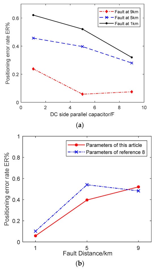
Figure 18.
The influence of system parameters on fault localization errors. (a) The influence of DC side capacitance parameters on fault location error rate; (b) The influence of line parameters on fault location error rate.
As can be seen from Figure 16, the impact of varying parameters on the accuracy of fault localization is minimal, with error rates remaining below 0.7%. Consequently, in pragmatic implementations, suitable capacitance and line parameters can be selected.
6. Comparison of Fault Location Performance of Different Algorithms
6.1. Convergence Comparison Between IRFO and RFO
A comparison of IRFO and RFO reveals that the former exhibits a substantially faster convergence rate in the localization of distribution network faults. The ensuing section will provide a visual comparison of the convergence of the two algorithms when a 5 km inter-pole short-circuit fault occurs on a direct current transmission line with the same parameter configuration. This comparison is illustrated in Figure 19.
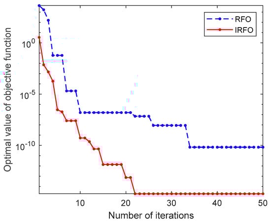
Figure 19.
Comparison of convergence between RFO and IRFO algorithms.
As can be seen from Figure 19, IRFO has significantly higher convergence speed than RFO, higher fault location accuracy, and smaller positioning error.
6.2. Comparative Analysis with Other Artificial Intelligence Algorithms
In this study, the improved red fox optimization (IRFO) algorithm, the particle swarm optimization (PSO) algorithm [36], and the gray wolf optimization (GWO) algorithm [37] are selected for a comparative analysis of fault location in DC distribution networks. It is noteworthy that the parameter values are maintained at a consistent level in IRFO.
Take the inter-electrode short-circuit fault of a 5 km DC line as an example. The comparison of the error rate of fault location and algorithm convergence for different faults is shown in Figure 20 and Figure 21.
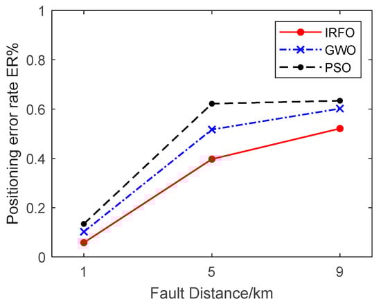
Figure 20.
Comparison of positioning error rates of different algorithms.
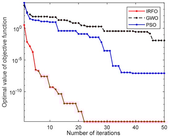
Figure 21.
Comparison of convergence situations of different algorithms.
As shown in Figure 20, the IRFO algorithm has much higher fault localization accuracy than other AI algorithms for the same number of populations and iterations.
As shown in Figure 21, the IRFO algorithm can achieve convergence within 25 iterations with the same number of populations and iterations. Compared with the PSO algorithm and the GWO algorithm, the IRFO algorithm has smaller optimal values of the objective function and higher accuracy with the same number of iterations.
As shown in Figure 22, the IRFO algorithm is computationally faster, taking only 3.7 ms for 50 iterations. The time used for iteration is second only to PSO algorithm and much lower than the GWO algorithm, with faster localization speed and higher robustness. In summary, the IRFO algorithm is used for fault localization with high localization speed, high localization accuracy, and good robustness. Precise localization can be achieved in the capacitor discharge stage, and the localization error rate is significantly lower than other artificial intelligence algorithms.
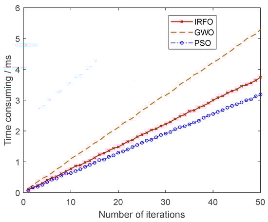
Figure 22.
Comparison of iteration consumption time of different artificial intelligence algorithms.
7. Conclusions
In this paper, an accurate fault localization scheme for multi-terminal DC distribution networks is proposed. Initially, the model encompasses inter-pole short-circuit faults and single-pole short-circuit faults. Subsequently, the voltage equations are established by collecting voltage data from both ends of the line to calculate the distance between the fault point and the protection installation location. The ensuing simulation experiments have yielded the following conclusions:
- The system demonstrates high fault localization accuracy and strong resistance to transition resistance. In the absence of transition resistance, the fault location error is maintained below 1%. For single-pole grounding faults, when the transition resistance reaches 100 Ω, the location error does not exceed 1.5%. In the case of inter-pole faults, even if the transition resistance reaches 5 Ω, the location error can still be controlled within 2%.
- The impact of low sampling frequency and data desynchronization on fault location is significantly reduced. In scenarios where the sampling frequency is limited, the fault voltage is addressed through adaptive interpolation, a process that effectively mitigates the error in fault localization. This, in turn, enables workers to promptly repair the faulty line and restore the power supply. Additionally, this approach reduces the financial investment required for sampling equipment. In scenarios involving abnormal and unsynchronized sampling data, the IRFO algorithm ensures the accurate and expeditious localization of faults, thereby facilitating the timely completion of the localization process.
- The applicability of the method is robust. The fault localization method is straightforward and depends exclusively on the voltage data at both ends of the faulted line. To illustrate this point, consider a fault at a distance of 5 km. In this scenario, IRFO demonstrates superior convergence speed and localization accuracy when compared with GWO, PSO, and RFO. This result underscores the efficacy and robustness of IRFO in practical applications.
Author Contributions
Conceptualization, Z.C.; methodology, Z.C.; investigation, Z.C. and Q.L.; resources, Q.L.; data curation, Z.C. and Q.L.; writing—original draft, Z.C.; writing—review and editing, Z.C. and Q.L. All authors have read and agreed to the published version of the manuscript.
Funding
This work was supported in part by the Hebei Province Key R&D Program project under grant 20314301D and, in part, by the State Grid Corporation of China’s technology project under grant kj2024-025.
Data Availability Statement
Data are contained within the article.
Conflicts of Interest
The authors declare no conflicts of interest.
References
- Satea, M.; Elsadd, M.; Zaky, M.; Elgamasy, M. Reliable High Impedance Fault Detection with Experimental Investigation in Distribution Systems. Eng. Technol. Appl. Sci. Res. 2024, 5, 17248–17255. [Google Scholar] [CrossRef]
- Fotopoulou, M.; Rakopoulos, D.; Trigkas, D.; Stergiopoulos, F.; Blanas, O.; Voutetakis, S. State of the Art of Low and Medium Voltage Direct Current (DC) Microgrids. Energies 2021, 14, 5595. [Google Scholar] [CrossRef]
- Shi, W.; Qu, J.; Luo, K.; Li, Q.; He, Y.; Wang, W. Research on high ratio new energy grid connection and operation development. China Eng. Sci. 2022, 24, 52–63. [Google Scholar] [CrossRef]
- Opiyo, N.N. A comparison of DC- versus AC-based minigrids for cost-effective electrification of rural developing communities. Energy Rep. 2019, 5, 398–408. [Google Scholar] [CrossRef]
- Zuo, X. Grid-connected technology operation of modern wind power new energy. J. Res. Sci. Eng. 2023, 5. [Google Scholar] [CrossRef]
- Huo, J.; Meng, R.; Li, S.; Liu, Q. Analysis and protection of inter pole short circuit faults in low-voltage DC distribution systems. Grid Clean Energy 2023, 39, 19. [Google Scholar]
- Nian, H.; Kong, L. Review of fault protection technology for DC microgrids. High Volt. Eng. 2020, 46, 2241–2254. [Google Scholar]
- Luo, Y.; Bai, W.; Shu, K.; Zhang, J.; Pei, Z.; Fan, T. Research on fault location of distribution network hybrid lines based on traveling wave method. J. Cent. South Univ. Natl. (Nat. Sci. Ed.) 2024, 43, 567–572. [Google Scholar]
- Lei, C.; Hao, L.; Dai, J.; Zhang, L.; Wang, X.; Cui, C.; Qi, J.; Tang, X. A review of fault location research on high-voltage direct current transmission lines. Power Syst. Prot. Control 2022, 50, 178–187. [Google Scholar]
- Zhang, B.; Tang, L.; Liang, X. Research on fault location of distribution network based on genetic particle swarm optimization. Comput. Technol. Autom. 2021, 40, 33–37. [Google Scholar]
- Li, R.; Gao, X.; Wang, C.; Yu, B.; Xu, Y. DC transmission fault location based on wavelet entropy feature fusion and ISSA-BiTCN. Sci. Technol. Eng. 2024, 24, 11303–11313. [Google Scholar]
- Lan, Z.; Yuan, Y.; He, D.; Zheng, J.; Yu, X. A fault location method for DC distribution networks based on current differential initial values. South. Power Grid Technol. 2023, 17, 109–116. [Google Scholar]
- Madhloom, J.K.; Abd Ghani, M.K.; Baharon, M.R. Enhancement to the Patient’s Health Care Image Encryption System, Using Several Layers of DNA Computing and AES (MLAESDNA). Period. Eng. Nat. Sci. 2021, 9, 928–947. [Google Scholar] [CrossRef]
- Beni, G.; Wen, J. Swarm intelligence in cellular robotic systems. In Robots and Biological Systems: Towards a New Bionics? Springer: Berlin/Heidelberg, Germany, 1993. [Google Scholar]
- Meng, C.; Yang, S.; Qian, X. Ship spare parts prediction based on red fox optimization support vector machine regression. J. Hefei Univ. Technol. (Nat. Sci. Ed.) 2025, 48, 25–31. [Google Scholar]
- Meng, C.; Li, G.; Peng, Y. Prediction of Remaining Life of Lithium Batteries Using Particle Filtering Based on Improved Red Fox Algorithm. Electron. Compon. Mater. 2025, 44, 184–191, 200. [Google Scholar]
- Cao, Z.; Li, F.; Zhou, X.; Liu, Z. Research on the Optimization of Frame Production Scheduling by Integrating NSGA-II and Red Fox Algorithm. Manuf. Technol. Mach. Tools 2025, 154–163. [Google Scholar] [CrossRef]
- Zhang, Y.; Fang, S.; Luo, G.; Liu, Y.; Hei, J. Fault location of multi-terminal DC network based on traveling wave attenuation theory. Sci. Technol. Eng. 2020, 20, 13240–13248. [Google Scholar]
- Wang, G.; Fan, C.; Huang, Y. A fault location method for multi terminal DC distribution networks with limited current reactors. J. Power Syst. Autom. 2023, 35, 87–96. [Google Scholar]
- Kouba, N.E.Y.; Menaa, M.; Hasni, M.; Tehrani, K.; Boudour, M. A novel optimized fuzzy-PID controller in two-area power system with HVDC link connection. In Proceedings of the 2016 International Conference on Control, Decision and Information Technologies (CoDIT), Saint Julian’s, Malta, 6–8 April 2016; pp. 204–209. [Google Scholar]
- Han, X.; Wang, M.; Jiang, J.; Xia, Y.; Ding, Y.; Qi, P. An active fault location scheme for DC distribution networks based on genetic annealing algorithm. Comput. Digit. Eng. 2023, 51, 273–276. [Google Scholar]
- He, D.; Xu, M.; Lan, Z.; Wang, W.; Zeng, J.; Yu, X. Transient characteristics analysis of grounding faults in medium voltage DC distribution networks containing distributed photovoltaics. Power Autom. Equip. 2023, 43, 43–50. [Google Scholar]
- Xu, Y.; Liu, J.; Fu, Y.; Wang, Y. A transient calculation method for circular DC systems based on fault models. Electr. Meas. Instrum. 2018, 55, 1–6. [Google Scholar]
- Li, M.; Jia, K.; Bi, T.; Yang, G.; Liu, Y.; Yang, Q. Distance measurement protection suitable for DC distribution networks. Power Syst. Technol. 2016, 40, 719–724. [Google Scholar]
- Mohammed, H.; Rashid, T. FOX: A FOX-inspired optimization algorithm. Appl. Intell. 2022, 53, 1030–1050. [Google Scholar] [CrossRef]
- ALRahhal, H.; Jamous, R. AFOX: A new adaptive nature-inspired optimization algorithm. Artif. Intell. Rev. 2023, 56, 15523–15566. [Google Scholar] [CrossRef]
- Cheng, X.; Li, X.; Ma, X. A method for battery fault diagnosis and early warning combining isolated forest algorithm and sliding window. Energy Sci. Eng. 2023, 11, 4493–4504. [Google Scholar] [CrossRef]
- Lin, X.; Xiao, Y.; Lei, Y.; Gu, Y.; Qian, B.; Tang, J.; Zhang, F. DC charging power measurement method based on wavelet threshold denoising and smoothing. China Meas. Test 2024, 50, 50–57. [Google Scholar]
- Zhou, X.; Zhang, Y.; Fang, Y.; Yang, H.; Xia, Y.; Wu, X.; Fan, D.; Sun, B. Research on sag measurement method of overhead transmission line based on fusion of similarity measure and Newton interpolation method. J. Electron. Meas. Instrum. 2023, 37, 221–229. [Google Scholar]
- Wang, K.; Zhao, Z.; Zhong, J.; Xu, F. Dynamic fault recovery strategy for distribution network based on improved simulated annealing genetic algorithm. Smart Power 2024, 52, 16–22. [Google Scholar]
- Xu, Y.; Hu, Z.; Dong, H. Fault localization of flexible DC distribution network based on grey comprehensive correlation degree. Acta Energiae Solaris Sin. 2023, 44, 324–331. [Google Scholar]
- Sun, G.; Shi, B.; Zhao, Y.; Li, S. Research on fault location and protection configuration of flexible DC distribution network based on MMC. Power Syst. Prot. Control 2015, 43, 127–133. [Google Scholar]
- Dhar, S.; Patnaik, R.K.; Dash, P.K. Fault detection and location of photovoltaic based DC microgrid using differential protection strategy. IEEE Trans. Smart Grid 2018, 9, 4303–4312. [Google Scholar] [CrossRef]
- Zhang, Z.; Fu, Y.; Wang, Y. Analysis of single pole grounding fault in DC transmission lines based on VSC. Mod. Electr. Power 2017, 34, 82–88. [Google Scholar]
- Muniappan, M. A comprehensive review of DC fault protection methods in HVDC transmission systems. Prot. Control Mod. Power Syst. 2021, 6, 1–20. [Google Scholar] [CrossRef]
- Wang, M.; Xu, Y. Fault Localization in Multi-Terminal DC Distribution Networks Based on PSO Algorithm. Electronics 2024, 13, 3420. [Google Scholar] [CrossRef]
- Luo, C. Research on Fault Section Localization of Distribution Network Based on Grey Wolf Algorithm. Master’s Thesis, Nanchang University, Nanchang, China, 2021. [Google Scholar]
Disclaimer/Publisher’s Note: The statements, opinions and data contained in all publications are solely those of the individual author(s) and contributor(s) and not of MDPI and/or the editor(s). MDPI and/or the editor(s) disclaim responsibility for any injury to people or property resulting from any ideas, methods, instructions or products referred to in the content. |
© 2025 by the authors. Licensee MDPI, Basel, Switzerland. This article is an open access article distributed under the terms and conditions of the Creative Commons Attribution (CC BY) license (https://creativecommons.org/licenses/by/4.0/).