Optimized Explainable Machine Learning Protocol for Battery State-of-Health Prediction Based on Electrochemical Impedance Spectra

Abstract

Monitoring the battery state of health (SOH) has become increasingly important for electric vehicles (EVs), renewable storage systems, and consumer gadgets. It indicates the residual usable capacity and performance of a battery in relation to its original specifications. This information is crucial for the safety and performance enhancement of the overall system. This paper develops an explainable machine learning protocol with Bayesian optimization techniques trained on electrochemical impedance spectroscopy (EIS) data to predict battery SOH. Various robust ensemble algorithms, including HistGradientBoosting (HGB), Random Forest, AdaBoost, Extra Trees, Bagging, CatBoost, Decision Tree, LightGBM, Gradient Boost, and XGB, have been developed and fine-tuned for predicting battery health. Eight comprehensive metrics are employed to estimate the model’s performance rigorously: coefficient of determination (R²), mean squared error (MSE), median absolute error (medae), mean absolute error (MAE), correlation coefficient (R), Nash–Sutcliffe efficiency (NSE), Kling–Gupta efficiency (KGE), and root mean squared error (RMSE). Bayesian optimization techniques were developed to optimize hyperparameters across all models, ensuring optimal implementation of each algorithm. Feature importance analysis was performed to thoroughly evaluate the models and assess the features with the most influence on battery health degradation. The comparison indicated that the GradientBoosting model outperformed others, achieving an MAE of 0.1041 and an R² of 0.9996. The findings suggest that Bayesian-optimized tree-based ensemble methods, particularly gradient boosting, excel at forecasting battery health status from electrochemical impedance spectroscopy data. This result offers an excellent opportunity for practical use in battery management systems that employ diverse industrial state-of-health assessment techniques to enhance battery longevity, contributing to sustainability initiatives for second-life lithium-ion batteries. This capability enables the recycling of vehicle batteries for application in static storage systems, which is environmentally advantageous and ensures continuity.

1. Introduction

Lithium-ion batteries are now a significant part of modern technology, used in many applications, such as EVs, ESS, and consumer electronics. In critical applications, these batteries lose their power over time, which shows up as a drop in capacity and a rise in impedance [1]. State of health (SOH) is a measure of the cell’s present state related to its fresh state. Moreover, health monitoring is important for the effective recycling of lithium-ion batteries, where batteries must be replaced when their capacity reduces below 80% [2]. An accurate evaluation of health is also vital for efficient recycling systems.

The primary condition of a battery is often evaluated by comparing its present capacity with its original rated capacity after aging. Typically, the approach to determine capacity, which involves continuous charge and discharge cycles, capacity decay, has become more challenging as a result of its energy inefficiency and time-consuming nature [3]. Battery health combines electrical data with machine learning to quickly and precisely evaluate battery condition. Thus, there is a critical necessity for procedures that can rapidly and efficiently assess battery health. Earlier methodologies that analyze charge/discharge data by analyzing the difference voltage, new capacity analysis, and Kalman filtering are inherently slow and inefficient, involving large data collection for the time being, which proves insufficient for rapid health state estimation [4].

Electrochemical impedance spectroscopy (EIS) has become useful in gradually obtaining internal battery data, as shown by various research studies [5]. This method involves applying low-amplitude AC impulses at various frequencies to the battery and evaluating the resulting signals, thereby improving understanding of the battery’s internal mechanisms. EIS is useful in finding the sources of battery degradation and has been crucial in the rise of health monitoring systems [6]. Battery research uses machine learning (ML) algorithms to estimate battery health through fundamental constraints such as temperature and voltage, with methods like KNN (K-Nearest Neighbors) and Decision Tree (DT) showing successful results [7]. Techniques like Principal Component Analysis, Convolutional Neural Network-Transformer, Beetle Antennae Search, Extreme Learning Machine, and advanced deep learning techniques help improve the monitoring of batteries in EVs and the recycling of energy wastage for SOH valuation [8,9]. Notably, all of these developments positively impact battery testing by increasing speed, accuracy, and environmental sustainability, while also improving the prediction of battery longevity under real-world scenarios. The prominent feature of tree-based models, such as Random Forest and gradient boosting models, is their capability to handle linear as well as nonlinear relationships for SOH estimation [10].

In this context, machine learning techniques show great performance in this domain, accurately identifying capacity degradation through variations in the impedance spectrum during battery aging for SOH estimation [11]. An Extreme Learning Machine (ELM) and Particle Swarm Optimization (PSO) technique is used to improve the estimation of SOH [3]. These techniques improve safety, perform properly in real-world applications, and contribute to increasing battery life through improved monitoring of both new and used batteries [4]. Similarly, a thorough evaluation analyzes more than 30 public lithium-ion battery datasets, emphasizing testing techniques and easily available research tools for SOH estimation [12]. For instance, gradient boosting decision trees have improved the predicted electric vehicle range to 0.7 km, although comparison analyses indicate that neural networks outperform conventional regression techniques in battery modeling [13]. Recurrent neural network (RNN) with long short-term memory (LSTM) has shown outstanding accuracy in estimating state of charge by effectively capturing temporal connections and adapting to various operating conditions for SOH estimation [14,15,16]. A GRU-based neural network approach is presented in [13] for the estimation of remaining useful life, achieving remarkable accuracy with a mean forecast error of less than 3%. Various ensemble techniques, such as extra tree, have been proposed to improve the learning capacity of these models. However, these studies primarily focus on evaluating machine learning techniques for battery management systems in high-power applications, such as EVs, based on differential voltage. They have successfully combined electrochemical impedance spectroscopy with time-domain variables to precisely assess battery health by applying weak AC signals, thereby improving the safety and cost aspects of energy systems for SOH estimation [17].

Additionally, modern approaches such as machine learning, temporal convolutional networks, and innovative frameworks employing Locally Sensitive K-Nearest Neighbors (LSKNN), Mixed-Integer Evolution Strategy (MIES), and Covariance-based Support Vector Gaussian Process Regression (CSVGPR) showed better precision in estimating battery degradation and remaining useful life compared to traditional methods for SOH estimation [18]. Therefore, a deep learning-based battery management system using Monte Carlo Cross-validation Protocol (MCCP) to forecast capacity provided superior results compared to conventional approaches with reduced error rates of EIS for determining battery health [19]. A neural network method incorporating LSTM networks with particle swarm optimization and attention mechanisms has shown exceptional accuracy for lithium-ion battery health management for SOH valuation [20]. An advanced deep learning approach that uses Fuzzy Oversampling-ELM and attention mechanisms to enhance the efficiency and precision of assessing the remaining useful life of batteries for SOH estimation is presented in [21]. A comparative health monitoring approach for battery management systems that accurately decreases estimation error issues and includes various indicators, while attaining outstanding precision with estimation errors around 3%, is presented in [22]. Nevertheless, the research focused primarily on identifying health indicators from complete impedance spectra, frequently missing the vital aspect of frequency range selection for SOH estimation [23]. This error may limit the study’s comprehensiveness, indicating a necessity for more research that would improve the precision of EIS for determining battery health [4]. This method evaluates newly developed methods for measuring impedance spectra over various frequency ranges. Contrary to conventional views, recording of global impedance spectra frequently requires several minutes, hence reducing the assumed advantage of rapid data collection associated with AC impedance spectra related to traditional voltage and current studies for SOH estimation [24].

By selecting frequencies that show strong correlations with battery degradation, we could improve the process and provide rapid diagnostics by measuring the value of AC impedance at specific frequencies [25]. An approach is developed using machine learning and ensemble methods for state-of-health prediction, tested with NASA datasets that show exceptional precision and stability of EIS for determining battery health [26]. A novel method for predicting battery lifespan combines support vector regression with particle filtering to model mechanisms of ageing and impedance degradation, with experimental results validating its accuracy and precision with SOH estimation [27]. All of these works combined represent significant improvements in battery health monitoring systems, especially regarding computational efficiency, predictive accuracy, and practical use in real-world battery management systems [28]. Therefore, An Improved Temporal Convolutional Network (ITCN) estimates lithium-ion battery health using multi-feature extraction from charging curves and capacity data, incorporating channel attention and residual shrinkage modules, achieving 1.47% prediction error [29]. They used a CNN-LSTM model with skip connection to estimate lithium-ion battery health using incremental capacity analysis and a feature selection algorithm, achieving RMSE below 0.004 on NASA and Oxford datasets by addressing neural network degradation [30]. A novel hybrid CNN and multi-head self-attention model estimates lithium iron phosphate battery health under fast-charging conditions using voltage-capacity data from an 80–97% SOC range, achieving 97% R² accuracy with transfer learning optimization [31].

Most current approaches, however, still rely on intricate model structures or extensive training requirements, which limit their applicability across a variety of battery chemistries and operating conditions. Additionally, many methods are not interpretable, making it difficult to determine which frequency bands or impedance characteristics have the greatest influence on SOH forecasts. Additionally, there is a significant gap in the development of transparent, reliable, and computationally efficient SOH prediction systems, as most studies do not integrate explainable machine learning methods or systematically optimize the EIS feature space.

Although many deep learning methods have been applied to battery health prediction, this study focuses on tree-based ensemble models because they are well-suited for tabular EIS data, require fewer samples, and offer better interpretability for physical analysis. This study proposes an optimized, understandable machine-learning framework for predicting lithium-ion battery SOH using EIS. Unlike other methods that mostly rely on full impedance spectra or deep learning architectures, the proposed method systematically tests ten advanced tree-based ensemble models that have been improved through Bayesian hyperparameter optimization. A significant contribution of this work is a frequency-importance evaluation strategy that finds the most important impedance features. This allows accurate SOH estimation with a smaller set of frequencies. This greatly speeds up both computation and diagnosis, making the method well-suited for battery management systems that need to operate in real time. Explainability analysis also shows which EIS features and operating conditions have the most significant effect on battery aging. The outcomes show that the suggested Bayesian-optimized ensemble method gives very accurate, precise, and fast SOH estimates. This makes it a good choice for embedded battery management system (BMS) applications and second-life energy storage deployments. The key contributions are summarized below.

▪

Developed a machine-learning framework that is optimized and easy to understand, using ten Bayesian-tuned tree-based ensemble models to precisely predict SOH of lithium-ion batteries from EIS data.

▪

Introduced a frequency-importance evaluation method that finds the most important impedance features. This facilitates accurate SOH estimation using a smaller set of EIS frequencies, speeding up diagnostics and making them more efficient.

▪

The method is good for real-time embedded BMS applications and second-life battery systems because it showed high transparency and computational efficiency through explainability analysis and optimized model design.

The remainder of the paper is organized as follows. Section 2 describes data analysis. Section 3 provides the materials and methods. Results and discussions are provided in Section 4. Finally, this work is summarized in Section 5.

2. Data Analysis

The experimental data were obtained from the Cavendish Laboratory at the University of Cambridge, UK. The experiment evaluated the aging of lithium batteries using Eunicell LIR2032 coin cells featuring LiCoO₂ cathodes and graphite anodes. Twelve batteries were assessed at three temperatures, 25 °C (25C01–25C08), 35 °C (35C01 and 35C02), and 45 °C (45C01 and 45C02), across 300–500 charge/discharge cycles per battery [11]. Electrochemical Impedance Spectroscopy (EIS) sizes were obtained at each cycle over nine charge/discharge states, applying frequencies ranging from 0.02 Hz to 20 kHz. To ensure analytical precision, the researchers used EIS data from batteries at “state V,” corresponding to a fully charged condition (100% SOC) after being isolated from direct current for 15 min. Eight distinct batteries (designated B1-B8) were chosen for examination. SOH was found by dividing the present capacity by the rated capacity of a fresh battery [1].

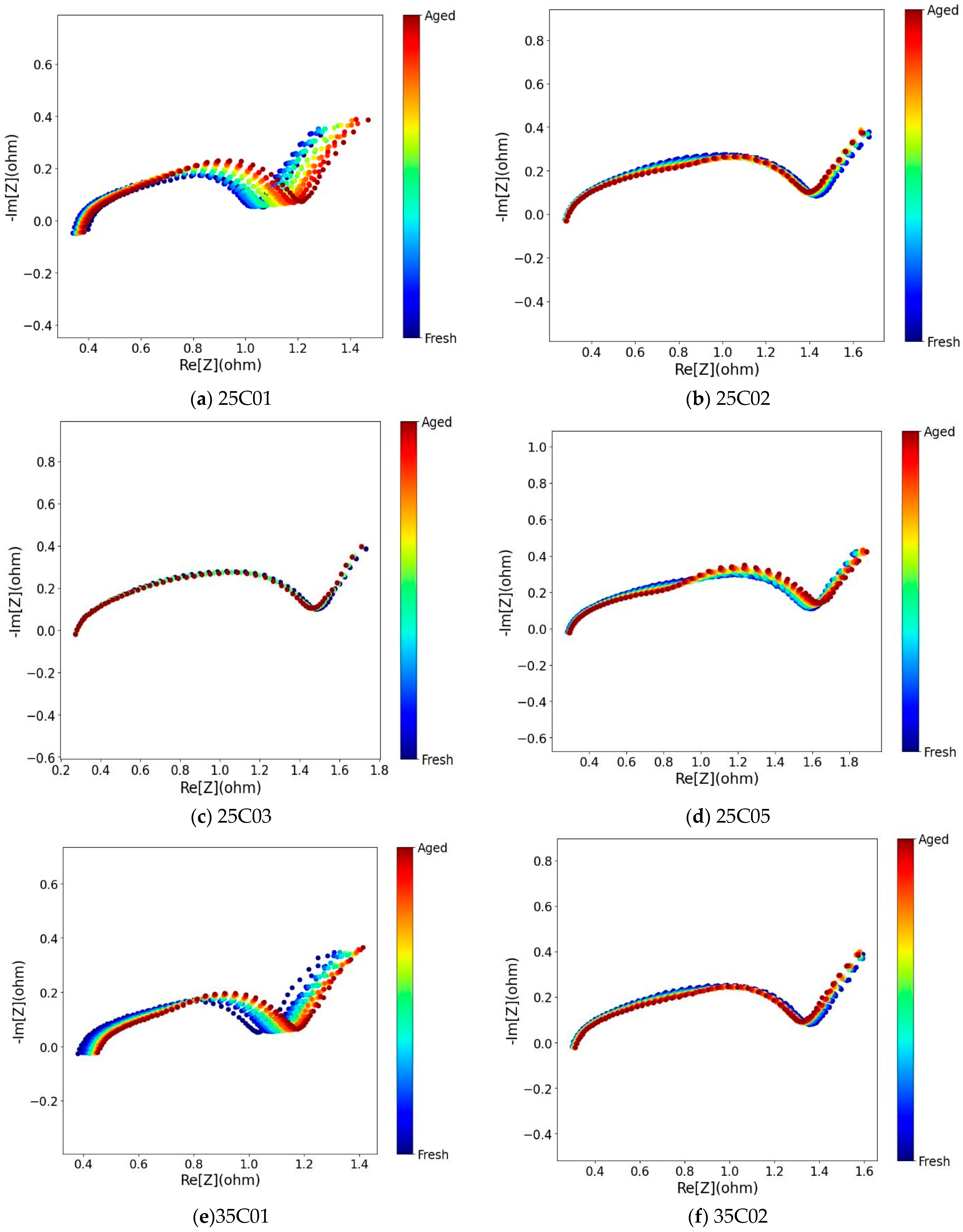
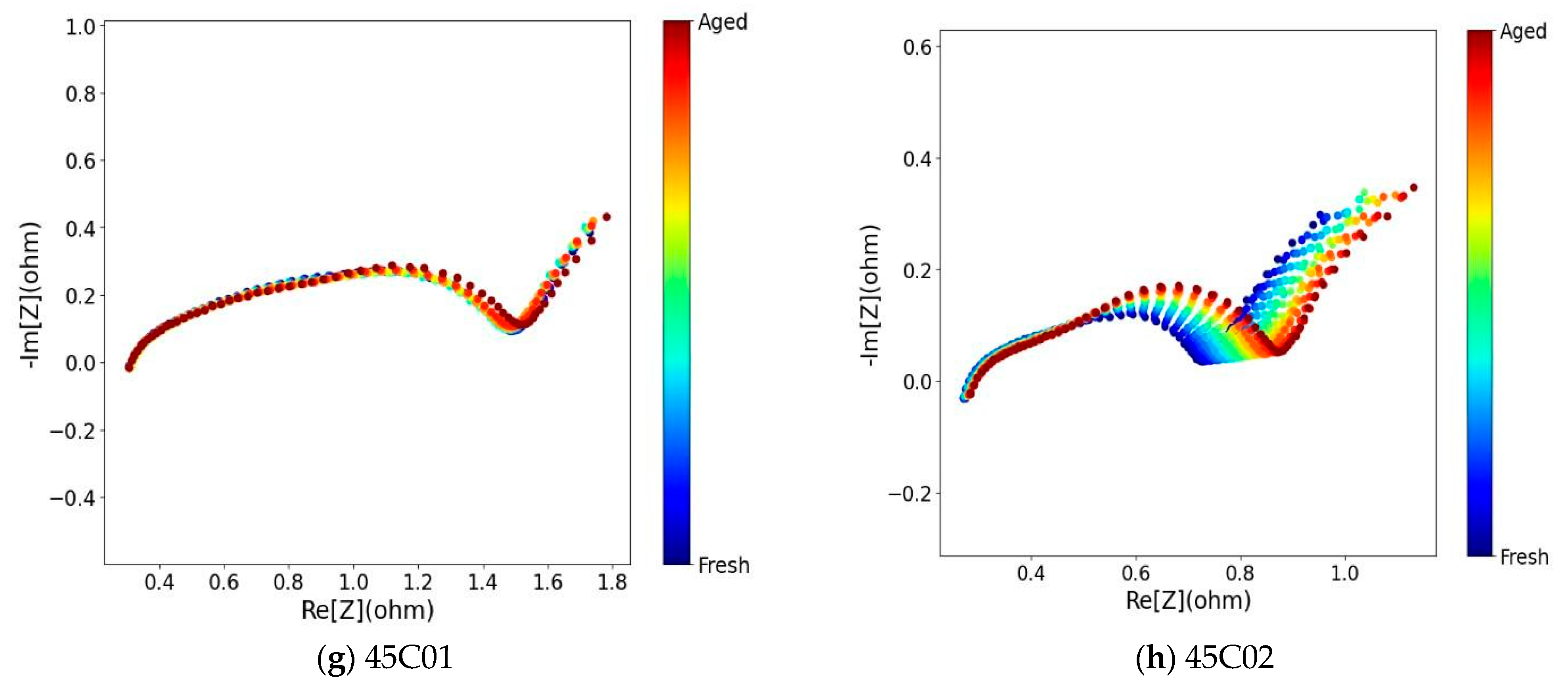
This Nyquist plot shows electrochemical impedance spectroscopy (EIS) data showing battery degradation from fresh (blue) to aged (red) states. Figure 1 shows real impedance on the x-axis and negative imaginary impedance on the y-axis, both measured in ohms for 25C01, 25C02, 25C03, 25C5, 35C01, 35C02, 45C01, and 45C02. Fresh batteries show lower impedance values with compact semicircular shapes, but aging continuously improves overall impedance and changes the curve features. The evolution from blue through green, yellow, orange to red demonstrates how internal resistance grows over battery lifetime. Capacity calibration was conducted at every odd cycle. The relationship between the capacity of all batteries and the number of cycles is depicted in Figure 1.

Finally, to remove ambiguity in feature interpretation, the 120 impedance features (Z1 to Z120) are clarified as representing the real and imaginary components of the 60 EIS frequency points listed in

Table 1. EIS frequency points.

Frequency Range	Actual Selected Frequency Point (Hz)
0.02–0.2 Hz	0.01999, 0.02528, 0.03192, 0.04042, 0.05102, 0.06443, 0.08153, 0.10309, 0.13007, 0.16452
0.2–2 Hz	0.20791, 0.26261, 0.33183, 0.41976, 0.53067, 0.67072, 0.84734, 1.07079, 1.35352, 1.70952
2–20 Hz	2.16054, 2.73547, 3.45686, 4.36941, 5.5173, 6.97545, 8.81772, 11.1448, 14.06813, 17.79613
20–200 Hz	22.48202, 28.40909, 35.93134, 45.3629, 57.36816, 72.51701, 91.6721, 115.77804, 146.35823, 185.05922
200 Hz–2 kHz	233.87738, 295.47278, 373.20856, 471.96338, 596.71857, 754.27557, 952.86591, 1203.8446, 1522.4358, 1923.1537
2 kHz–20 kHz	2430.7778, 3070.9827, 3881.2737, 4905.291, 6217.2461, 7835.48, 9909.4424, 12,516.703, 15,829.126, 20,004.453

, spanning 0.02 Hz to 20 kHz. Each frequency contributes two sequential features, Re(Z) and Im(Z), across the Z labels. For example, Z94 and Z108, identified as highly influential by SHAP, correspond to the imaginary impedance at mid- and high-frequency points within the 20 to 200 Hz and 200 Hz to 2 kHz bands, respectively. These frequency regions are closely associated with charge-transfer resistance, interfacial kinetics, and mobility limitations, which evolve with aging and thus serve as strong electrochemical indicators for SOH prediction.

One of the key diagnostic techniques for battery evaluation is EIS, which characterizes the system by applying a small AC excitation across a wide frequency range, typically from microhertz to kilohertz. The response signal, usually a voltage response to current input, is collected simultaneously. The collected data allows the calculation of complex impedance in the frequency domain. Based on this analysis, it is then possible to create a Nyquist plot from the impedance spectrum, using the resistor part or fundamental part on the horizontal axis and the negative imaginary part on the vertical axis. It allows for analysis of internal battery procedures, such as ohmic internal resistance, charge transfer, solid electrolyte interface layer, and double-layer capacitance, among others. These methods change as the battery ages, suggesting that EIS could serve as a reliable, objective metric for characterizing the battery’s aging state.

$$T={\displaystyle \sum _{i=1}^n\frac{1}{{{\displaystyle f}}_i}}\times m$$

(1)

Frequency intervals are presented in Table 1; a single impedance spectrum measurement consumes approximately 239.5 s, where T designates the calculated total duration for single EIS measurement, m indicates the number of sine wave cycle replications at each frequency, n signifies the overall quantity of frequency points (n = 60), and fi expresses the frequency value of the AC signal frequency point, as specified in Table 1 [1].

The SOH of a battery is determined by dividing its current capacity by its rated capacity. To reduce complex calculations and eliminate overfitting, the generated experimental data were randomized by the equations below.

$${{\displaystyle X}}_{norm} = {\displaystyle \frac{{{\displaystyle X}}_i-{{\displaystyle X}}_{\min }}{{{\displaystyle X}}_{\max } - {{\displaystyle X}}_{\min }}}$$

(2)

$$SOH={\displaystyle \frac{{{\displaystyle Q}}_{now}}{{{\displaystyle Q}}_{new}}}\times 100\%$$

(3)

where Xi is any datum, X_min is minimum value, X_max is maximum value, Q_now is the current capacity, and Q_new is capacity at fresh condition.

3. Materials and Methods

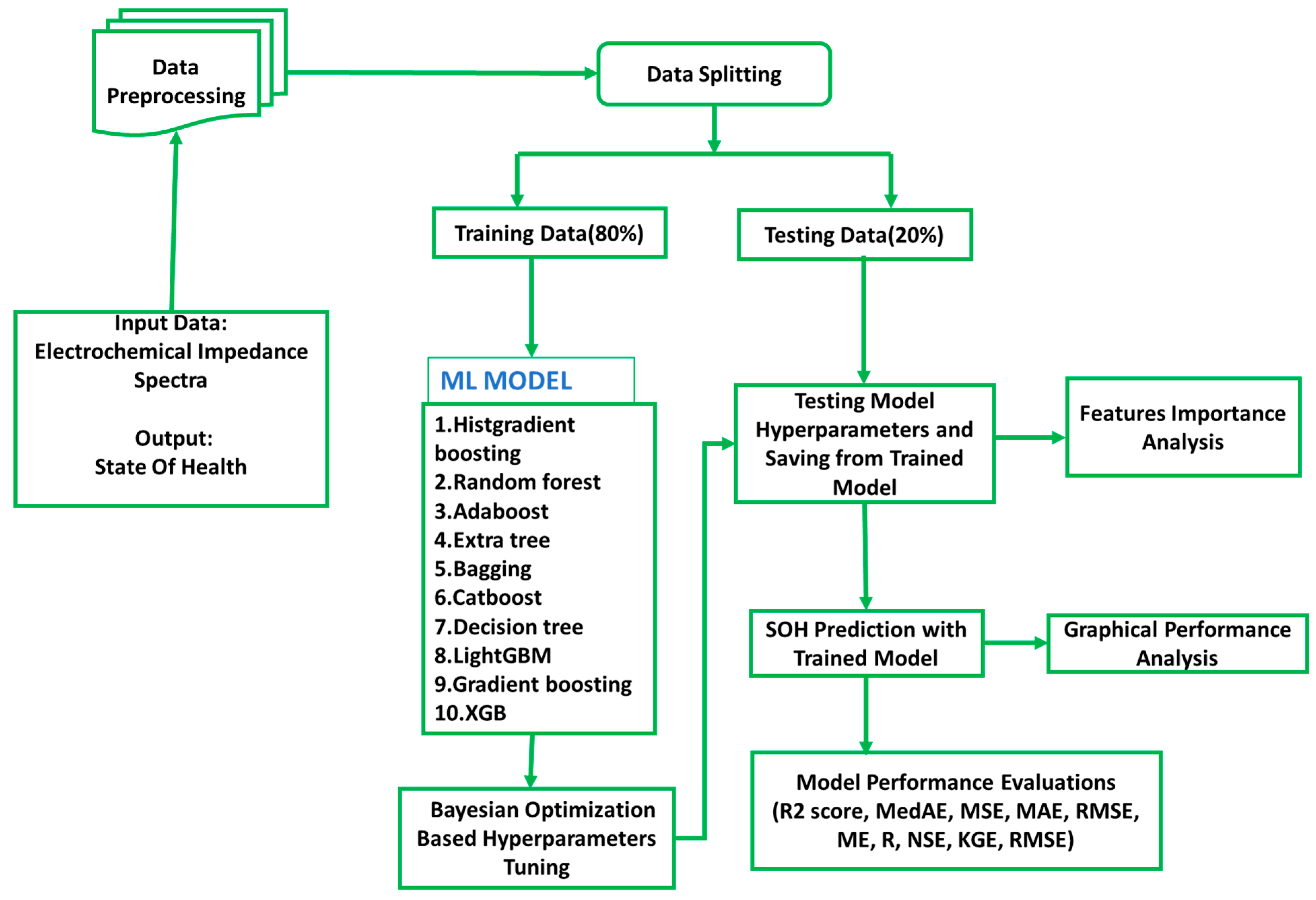
The methodological framework developed in this study is depicted in Figure 2, which delineates the comprehensive workflow for predicting battery SOH through EIS. This section delineates each phase of the process, encompassing data preprocessing, model selection, Bayesian optimization for hyperparameter tuning, and performance evaluation utilizing a range of machine learning algorithms. Additionally, the statistical metrics employed for model evaluation, including R², MSE, MAE, RMSE, ME, R, NSE, and KGE, are elucidated to facilitate a thorough comprehension of the quantitative assessment of prediction accuracy and robustness.

As shown in Figure 2, ten tree-based ML models were evaluated for battery SOH prediction, including HGB, RF, AdaBoost, ET, Bagging, CatBoost, DT, Light GBM, Gradient Boosting, and XG Boost. The dataset was divided using a random sample-based split, where individual EIS measurements from all batteries were randomly assigned to the training and test sets. Although this approach is common in prior EIS-based studies, it does not explicitly account for battery-wise or cycle-wise separation, which may lead to optimistic estimates of generalization. The training set was used to build the models, while the testing set evaluated their generalization performance. Bayesian optimization was applied to fine-tune the hyperparameters of each algorithm. The Bayesian approach systematically explores different parameter combinations to improve model performance. Each model’s effectiveness was assessed using the independent test dataset to ensure reliable predictions on unseen data. This methodology ensures robust model development and fair comparison between different tree-based ensemble algorithms for battery SOH assessment applications. The search was conducted over the hyperparameter ranges listed in

Table 2. Complete Bayesian optimization-based hyperparameters.

Model	Key Parameters	Search Range
HistGradientBoosting	max_iter	[50, 1000]
	learning_rate	[0.001, 0.3]
	max_depth	[3, 15]
	max_leaf_nodes	[15, 127]
	l2_regularization	[0, 10]
AdaBoost	n_estimators	[50, 1000]
	learning_rate	[0.001, 2.0]
	algorithm	[‘SAMME’, ‘SAMME.R’]
Extra Trees	n_estimators	[50, 500]
	max_ depth	[5, 30]
	min_sample_split	[2, 20]
	min_sample_leaf	[1, 10]
	max_features	[0.3, 1.0]
Random forest	n_estimators	[5, 500]
	max_depth	[5, 30]
	min_samples_split	[2, 20]
Bagging	n_estimators	[10, 300]
	max_samples	[0.5, 1.0]
	max_features	[0.5, 1.0]
Decision tree	max_depth	[3, 30]
	min_samples_split	[2, 50]
	max_features_leaf	[1, 20]
	max_features	[0.3, 1.0]
Catboost	depth	[4, 10]
	l2_leaf_reg	[1, 10]
	bagging_temperature	[0, 1]
LightGBM	num_leaves	[15, 127]
	learning_rate	[0.001, 0.3]
	min_child_samples	[5, 50]
Gradientboosting	n_estimators	[50, 1000]
	learning_rate	[0.001, 0.3]
	max_depth	[3, 15]
	subsample	[0.6, 1.0]
XGBoost	n_estimators	[50, 1000]
	learning_rate	[0.001, 0.3]
	gamma	[0, 1.0]
	colsample_bytree	[0.5, 1.0]

, including n_estimators, max_depth, learning_rate, min_samples_split, min_samples_leaf, subsample, and max_features. The optimization employed the Expected Improvement (EI) acquisition function with one random initialization point and three sequential optimization iterations, which provided an efficient balance between performance and computational cost.

Figure 2 also shows the methodological contribution of this study, which combines explainable machine learning with optimized EIS-based feature analysis for SOH prediction. In contrast to more traditional methods, the proposed framework combines model explainability through feature-importance analysis. This allows determining the impedance frequencies that have the most significant impact on SOH estimation. In addition, the methodology incorporates a comprehensive graphical performance evaluation, which enables a visual comparison of the model’s behavior across key statistical variables and supports the interpretability of prediction patterns. This framework provides a unified, systematic, and interpretable pipeline to improve diagnostic accuracy and enable data-driven decision-making in advanced battery management systems. It accomplishes this by merging Bayesian-optimized tree-based models with transparent evaluation methodologies.

3.1. HistGradientBoost (Histogram-Based Gradient Boosting)

HGB is a histogram-based gradient boosting technique that categorizes continuous features into discrete bins to accelerate training. It uses histogram-based techniques to effectively identify optimal splits and provides native support for missing values. The technique optimizes speed and precision using histogram statistics rather than precise feature values [32]. Predicted output is given by the following equation.

$$\widehat{y } ={\displaystyle {\sum }_{t=1^T }{{\displaystyle \gamma }}_t}·{{\displaystyle h}}_t\left(x\right)$$

(4)

where γ_t denotes the learning rate for the t-th tree, h_t(x) signifies the prediction of the t-th tree, and T is the total number of trees.

3.2. Random Forest

RF estimates use the mean of individual tree predictions for regression tasks or the total number of votes for classification tasks. It integrates bootstrap accumulating with random feature selection at each split, resulting in varied trees that continually offer accurate predictions with reduced variance [33]. The prediction equation for RB is as follows.

$$\widehat{y} =\left({\displaystyle \frac{1}{\beta }}\right){\displaystyle {\sum }_{\beta =1^{\beta }} {{\displaystyle T}}_{\beta }}\left(x\right)$$

(5)

where T_β(x) is the prediction of decision tree b, and B is the total number of trees in the forest.

3.3. AdaBoost (Adaptive Boosting)

AdaBoost is an adaptive boosting technique that continuously uses weak learners on weighted datasets. It increases the weights of misclassified cases and reduces the weights of accurately classified ones. Each subsequent weak learner focuses more on the examples that were incorrectly predicted by previous learners, leading to improved performance on difficult cases [34]. The prediction equation for AdaBoost is as follows.

$$\widehat{y} =sign\left({\displaystyle {\sum }_{t=1^T}{{\displaystyle \alpha }}_t·{{\displaystyle h}}_t\left(x\right)}\right)$$

(6)

where α_t = (1/2)ln((1 − ε_t)/ε_t) is the weight of the t-th weak learner, ε_t is the weighted error rate, and h_t(x) is the t-th weak learner’s prediction.

3.4. Extra Trees (Extremely Randomized Trees)

ET generates ensembles of decision trees by including more randomness in both feature selection and split threshold determination. Instead of identifying the optimal split for each feature, it randomly determines split thresholds, hence further eliminating variation while having low bias. This method results in rapid training and frequently improved generalization [35]. The prediction equation for ET is as follows.

$$\widehat{y} =\left({\displaystyle \frac{1}{k}}\right){\displaystyle {\sum }_{k=1^k}{{\displaystyle T}}_K\left(x\right)}$$

(7)

where T_k(x) is the prediction from the k-th extremely randomized tree, and K is the total number of trees in the ensemble.

3.5. Bagging

Bagging is an ensemble technique that integrates several models trained on various bootstrap samples of the original dataset. It reduces variance by averaging predictions from several weak learners, hence reducing the robustness of the final model and reducing its susceptibility to overfitting. Each model is trained individually on a randomly selected portion of the training data with replacement [36].

$$\widehat{y} =\left({\displaystyle \frac{1}{M}}\right){\displaystyle {\sum }_{i=1^M}{{\displaystyle h}}_i}\left(x\right)$$

(8)

where M is the number of bootstrap samples, h_i(x) is the prediction from the i-th model, and ŷ is the final averaged prediction.

3.6. CatBoost

CatBoost is a gradient boosting technique that inherently accommodates category information without necessitating preprocessing. It employs ordered boosting and symmetric trees to mitigate overfitting and enhance generalization. The technique constructs trees in succession, with each tree rectifying faults from prior iterations while preserving statistical efficiency via ordered target statistics [37]. The prediction equation for CatBoost is as follows.

$$\widehat{y} ={\displaystyle {\sum }_{i=1^M}{{\displaystyle \alpha }}_1}·{{\displaystyle h}}_i\left(x\right)$$

(9)

where α_i are the weights for each tree, h_i(x) are individual tree predictions, and M is the number of boosting iterations.

3.7. Decision Tree

Decision trees predict results by continuously splitting the input data according to feature values. Every internal node represents an evaluation of a feature, each branch shows the result of the evaluation, and each leaf node provides a class label or predicted value. The tree structure serves as simple rules for decision-making [10]. DT predicted output is given by the equation below.

$$\widehat{y} ={\displaystyle {\sum }_1\epsilon leaves {{\displaystyle c}}_1} · I\left(x\in {{\displaystyle R}}_1\right)$$

(10)

where c_l is the constant prediction value in leaf l, I(x ∈ R_l) is an indicator function that equals 1 if input x falls in region R_l, and 0 otherwise.

3.8. Light GBM

LightGBM is an efficient gradient boosting framework that uses HB techniques to enhance training speed and reduce memory used. It uses leaf-wise tree evolution rather than level-wise growth, which provides better precision with fewer iterations. The algorithm contains fundamental support for categorical features and handles missing data effectively [38]. LightGBM prediction is given by the equation below.

$$\widehat{y} = {\displaystyle {\sum }_{t=1^T}{{\displaystyle f}}_t}\left(x\right)$$

(11)

where f_t(x) represents the t-th tree prediction and T is the total number of trees. The objective function includes regularization terms to control overfitting.

3.9. Gradient Boosting

Gradient boosting builds models in order, with each subsequent model trained to address the residual errors of the initial ensemble. Each weak learner focused on the data severely predicted by recent models, resulting in improved overall performance [38]. GB’s predicted output is given by the equation below.

$$\widehat{y} = {{\displaystyle F}}_0\left(x\right)+{\displaystyle {\sum }_{m=1^M} {{\displaystyle \gamma }}_m}· {{\displaystyle h}}_m\left(x\right)$$

(12)

where F₀(x) is the initial prediction, γ_m is the learning rate for the m-th iteration, h_m(x) is the m-th weak learner, and M is the total number of iterations.

3.10. XGBoost (Extreme Gradient Boosting)

XGBoost is an optimization approach organized similarly to GBDT. It constructs the tree model sequentially, and every tree will try to eliminate residuals of the prior iteration on target. It offers a new tree method to decrease the target function at each time [32]. The XGBoost objective function at iteration t is given by the equation below.

$${{\displaystyle L}}^{\left(t\right)} ={\displaystyle {\sum }_{i=1^n}\left({{\displaystyle y}}_i , {{{\displaystyle \widehat{y}}}_i}^{(t-1)} + {{\displaystyle f}}_t\left({{\displaystyle x}}_i\right)\right)} + \mathrm{\Omega }\left({{\displaystyle f}}_t\right)$$

(13)

where l is the loss function, Ω is the regularization span that controls the complexity of the model, y_i is the true value, ŷ_i^(t−1) is the prediction from previous iteration, and f_t(x_i) is the new tree prediction. The hyperparameter ranges for different models are listed in Table 2.

3.11. Statistic Performance Analysis

Several statistical measures, including MAPE, KGE, R2, MedAE, MAE, NSE, RMSE, and MSE, as defined by equations below, were employed to assess the model’s predictive performance.

3.11.1. Coefficient of Determination

The coefficient of determination is given by the following equation. This equation represents the proportion of variance in the dependent variable that is predictable from the independent variable(s). Values range from 0 to 1 (or negative for poor models), where 1 indicates perfect prediction.

$$R^2 = 1-{\displaystyle \frac{{{\displaystyle \sum _{i=1}^n\left({{\displaystyle y}}_i-{{\displaystyle \widehat{y}}}_i\right)}}^2}{{\displaystyle \sum _{i=1}^n{\left({{\displaystyle y}}_i-{{\displaystyle \overline{y}}}_i\right)}^2}}}$$

(14)

where $y_i$ is the actual value, $y_i$ is the predicted value, $y$ is the mean of actual values, n is the number of observations, R² values range from 0 to 1, with higher values representing improved model performance.

3.11.2. Mean Absolute Percentage Error (MAPE)

The average of absolute percentage errors between predicted and actual values. It expresses accuracy as a percentage, making it scale-independent, and is given by the equation below.

$$MAPE={\displaystyle \frac{100}{n}}{\displaystyle \sum _{i=1}^n\left|\frac{{{\displaystyle y}}_i-{{\displaystyle \widehat{y}}}_i}{{{\displaystyle y}}_i}\right|}$$

(15)

3.11.3. Nash–Sutcliffe Efficiency (NSE)

NSE is given by the equation below. It compares model performance to using the mean of observed data as a predictor. Values above 0 indicate the model performs better than the mean; values near 1 indicate excellent performance.

$$NSE=1-{{\displaystyle \frac{{\displaystyle \sum _{i=1}^n\left({{\displaystyle y}}_i-{{\displaystyle \widehat{y}}}_i\right)}}{{\displaystyle \sum _{i=1}^n{\left({{\displaystyle y}}_i-{{\displaystyle \overline{y}}}_i\right)}^2}}}}^2$$

(16)

NSE is similar to R², and it shows how well the plot of observed versus simulated data fits the 1:1 line. The denominator is the total change of the observed data.

3.11.4. Kling–Gupta Efficiency (KGE)

KGE is another statistical performance indicator given by the equation below. It addresses some limitations of NSE by treating bias and variability errors more evenly.

$$KGE=1-\sqrt{{\left(r-1\right)}^2+{\left(\alpha -1\right)}^2+{\left(\beta -1\right)}^2}$$

(17)

where

$$r={\displaystyle \frac{{\displaystyle \sum _{i=1}^n\left({{\displaystyle y}}_i- \overline{y}\right)\left({{\displaystyle \widehat{y}}}_i- \widehat{\overline{y}}\right)}}{ \sqrt{{\displaystyle \sum _{i=1}^n{\left({{\displaystyle y}}_i-\overline{y}\right)}^2 }} \sqrt{{\displaystyle \sum _{i=1}^n{\left({{\displaystyle \widehat{y}}}_i- \overline{\widehat{y}}\right)}^2}}}}$$

r is the linear correlation coefficient, α is the ratio of the standard deviation of the predicted values to that of the observed ones, and β is similarly the ratio of the mean of the predicted values to the observed ones.

$$\alpha ={\displaystyle \frac{\partial \widehat{y}}{\partial y}}, \beta ={\displaystyle \frac{\mu \widehat{y}}{\mu y}}$$

3.11.5. Median Absolute Error (MedAE)

The median of absolute differences between predicted and actual values is more robust to outliers than MAE.

$$MedAE=median\left(\left|{{\displaystyle y}}_i-{{\displaystyle \widehat{y}}}_i\right|\right)$$

(18)

3.11.6. Mean Absolute Error (MAE)

The average of absolute differences between predicted and actual values measures the average magnitude of errors without considering their direction.

$$MAE={\displaystyle \frac{1}{n}}{\displaystyle \sum _{i=1}^n\left|{{\displaystyle y}}_i-{{\displaystyle \widehat{y}}}_i\right|}$$

(19)

3.11.7. Mean Squared Error (MSE)

MSE is the average of the squared differences between predicted and actual values, which is given by the equation below. It penalizes larger errors more heavily than MAE.

$$MSE={\displaystyle \frac{1}{n}}{{\displaystyle \sum _{i=1}^n\left({{\displaystyle y}}_i-{{\displaystyle \widehat{y}}}_i\right)}}^2$$

(20)

3.11.8. Root Mean Squared Error (RMSE)

The square root of MSE returns the error metric to the original units of the data and is given by the equation below. It is sensitive to outliers.

$$RMSE=\sqrt{{\displaystyle \frac{1}{n}}{{\displaystyle \sum _{i=1}^n\left({{\displaystyle y}}_i-{{\displaystyle \widehat{y}}}_i\right)}}^2}$$

(21)

4. Results and Discussion

This section presents a comprehensive evaluation of the performance of ten Bayesian-optimized tree-based machine learning (ML) algorithms for predicting the battery State of Health (SOH) using electrochemical impedance spectroscopy (EIS) data. The models include HistGradientBoosting (HGB), Random Forest (RF), AdaBoost (AB), Extra Trees (ET), Bagging (B), CatBoost (CB), Decision Tree (DT), LightGBM (LGBM), Gradient Boosting (GB), and XGBoost (XGB). Model performance was quantified using statistical indices such as R², MAE, MSE, NSE, KGE, and RMSE for both training and testing datasets, as summarized in

Table 3. Performance metrics for various investigated ML models.

MODEL	R2 Score	MEDAE	MSE	MAPE	MAE	ME	R	NSE	KGE	RMSE
HGB	0.9979	0.1787	0.2044	0.0035	0.2689	5.3198	0.9990	0.9978	0.9932	0.4521
	0.9942	0.4224	0.5531	0.0072	0.5423	4.9539	0.9971	0.9942	0.9955	0.7437
RF	0.9980	0.0832	0.1941	0.0022	0.1767	5.8390	0.9991	0.9979	0.9881	0.4406
	0.9978	0.1860	0.2074	0.0038	0.2886	3.9104	0.9989	0.9978	0.9911	0.4555
AD	0.9992	0.0471	0.0790	0.0013	0.1027	4.6767	0.9996	0.9992	0.9921	0.2810
	0.9973	0.1850	0.2526	0.0041	0.3128	3.7524	0.9987	0.9973	0.9941	0.5026
ET	0.9987	0.1293	0.1269	0.0016	0.1234	4.6767	0.9994	0.9987	0.9916	0.3558
	0.9987	0.1293	0.1269	0.0029	0.2147	2.9397	0.9993	0.9987	0.9939	0.3562
B	0.9961	0.1498	0.3728	0.0037	0.2892	7.0065	0.9982	0.9960	0.9841	0.6106
	0.9964	0.2522	0.3441	0.0051	0.3844	4.7362	0.9982	0.9963	0.9901	0.5866
CB	0.9987	0.1783	0.1274	0.0030	0.2318	4.6767	0.9994	0.9987	0.9939	0.3569
	0.9966	0.3045	0.3271	0.0054	0.4101	4.8281	0.9983	0.9965	0.9939	0.5719
DT	0.9893	0.5427	1.0292	0.0093	0.7141	8.6334	0.9946	0.9891	0.9882	1.0145
	0.9817	0.7017	1.7394	0.0118	0.8904	11.8256	0.9910	0.9817	0.9907	1.3189
LGBM	0.9987	0.1121	0.1230	0.0023	0.1822	4.6767	0.9994	0.9987	0.9921	0.3508
	0.9962	0.3100	0.3581	0.0056	0.4194	3.3839	0.9981	0.9962	0.9931	0.5984
GB	0.9993	0.0578	0.0715	0.0013	0.1041	4.6767	0.9996	0.9992	0.9933	0.2675
	0.9960	0.2868	0.3782	0.0054	0.4061	4.0960	0.9980	0.9960	0.9955	0.6149
XGB	0.9992	0.0710	0.0784	0.0015	0.1194	4.6767	0.9996	0.9992	0.9938	0.2801
	0.9956	0.3444	0.4214	0.0061	0.4631	3.2628	0.9978	0.9955	0.9912	0.6491
		Training Data			Testing Data

.

4.1. Model Performance Evaluation

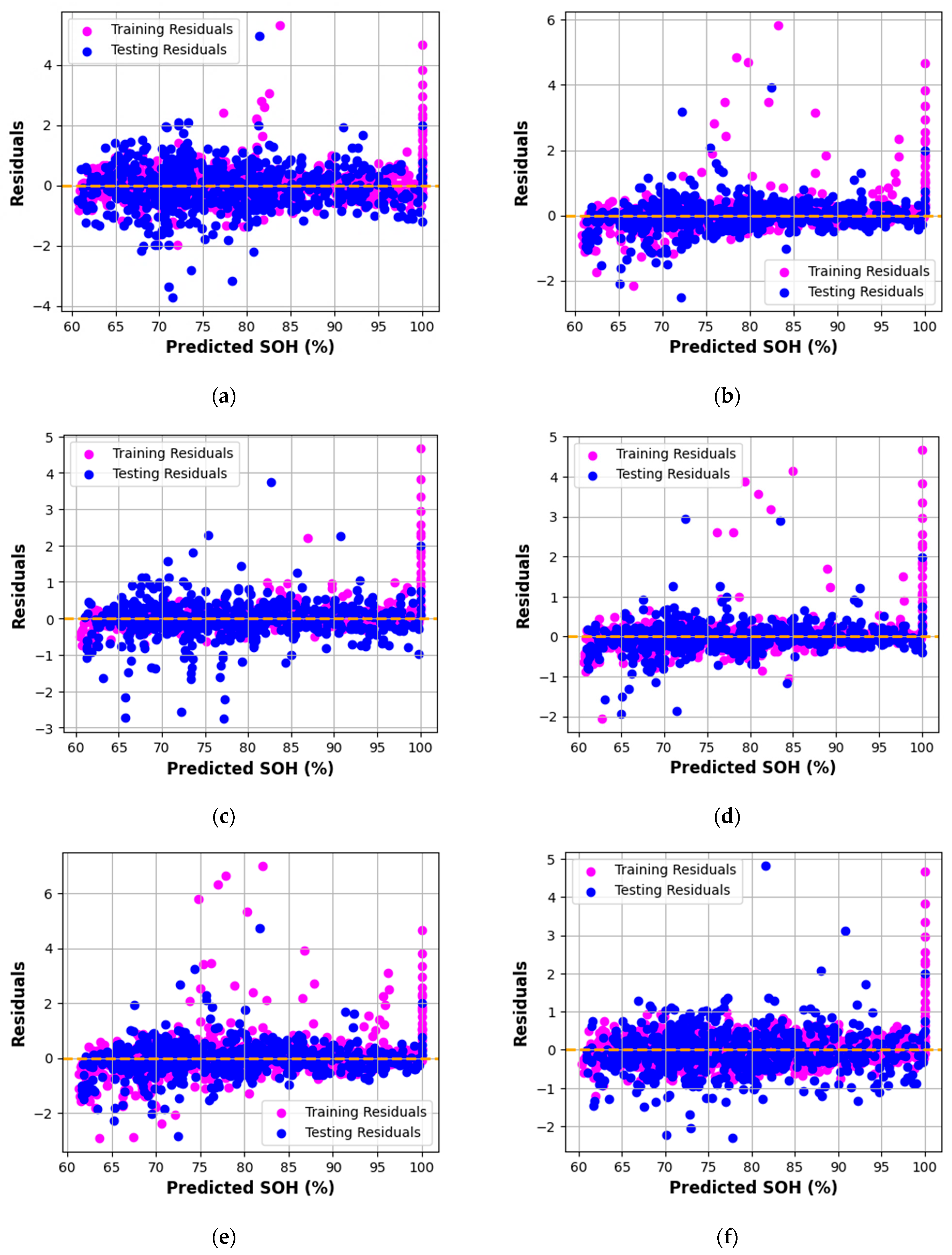
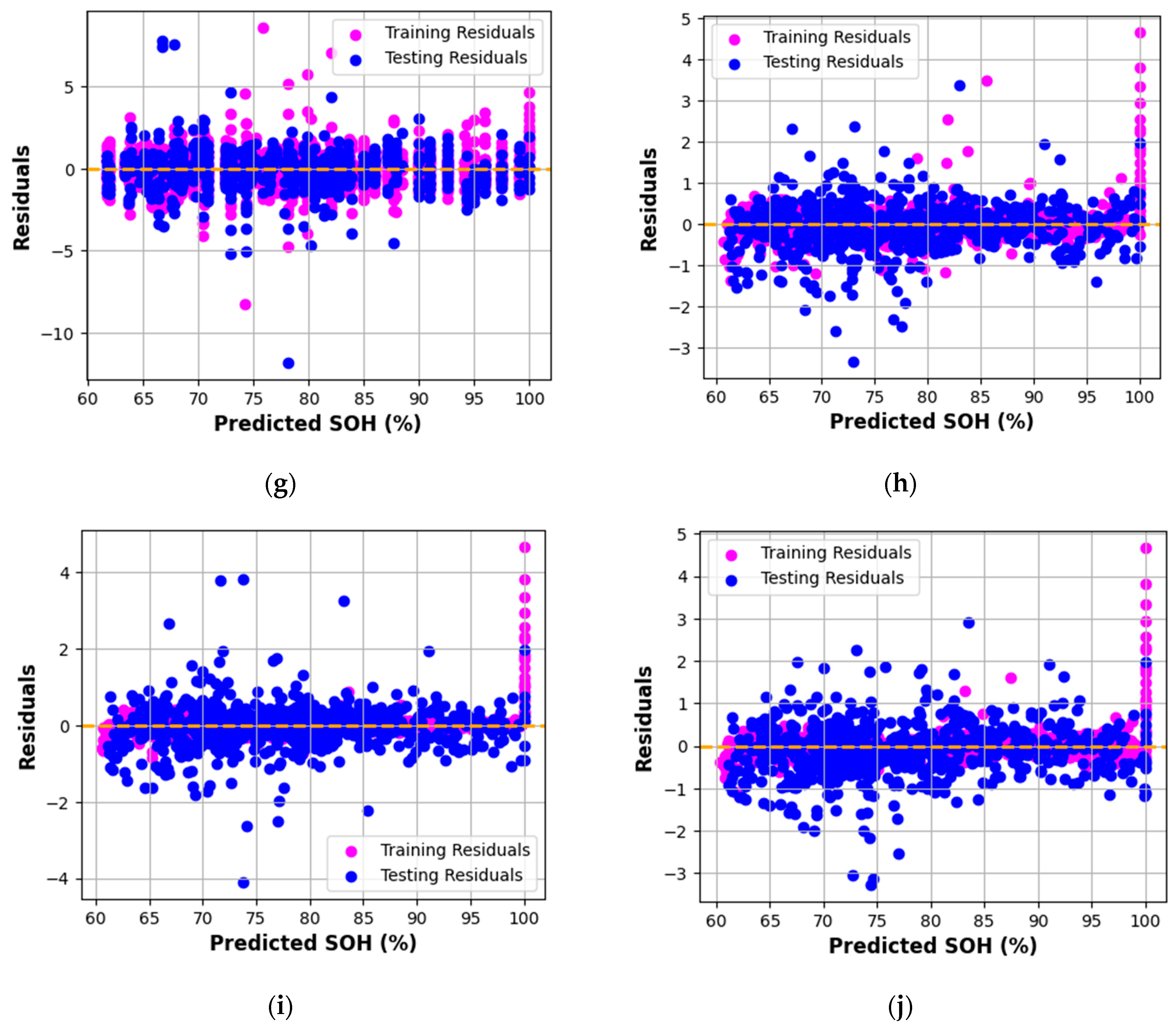
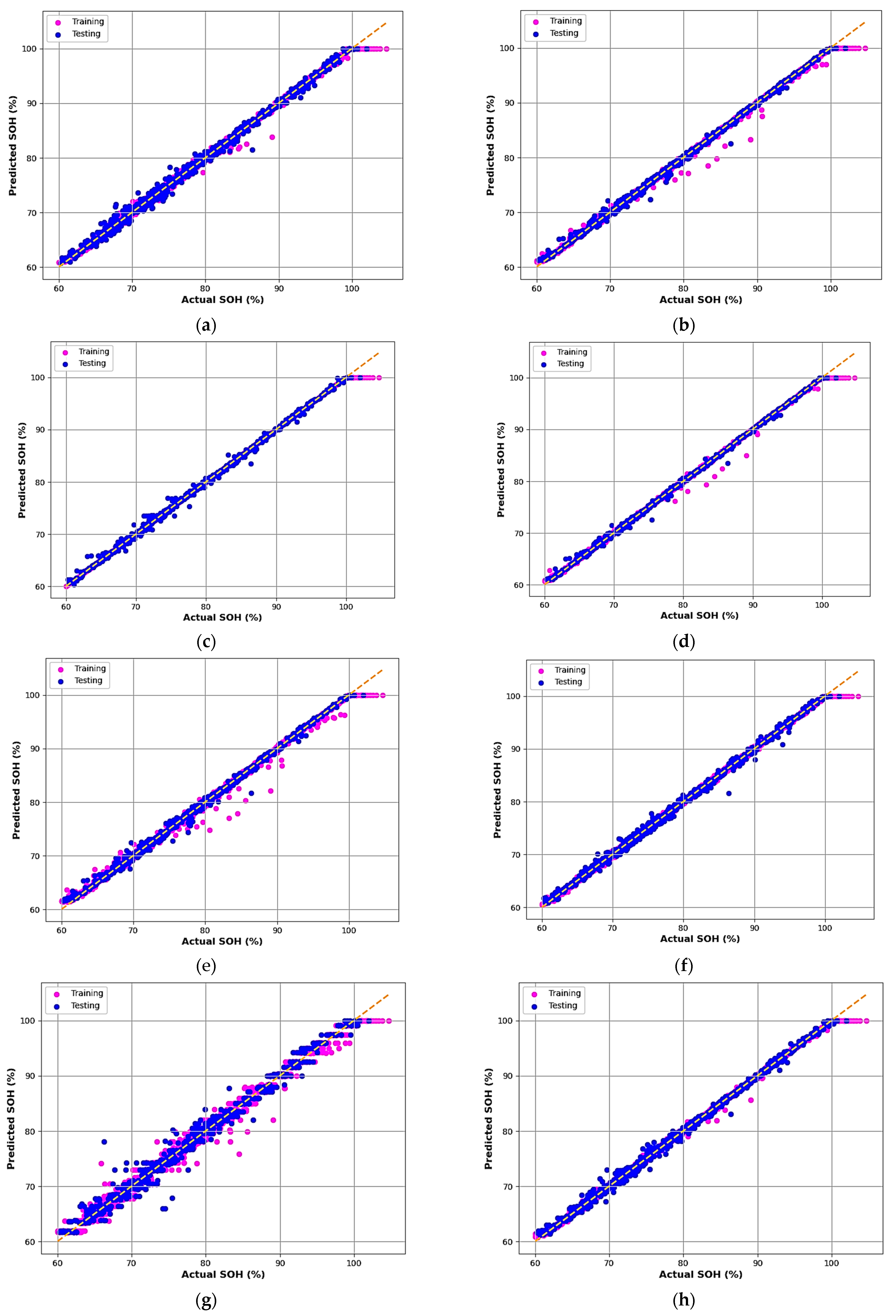
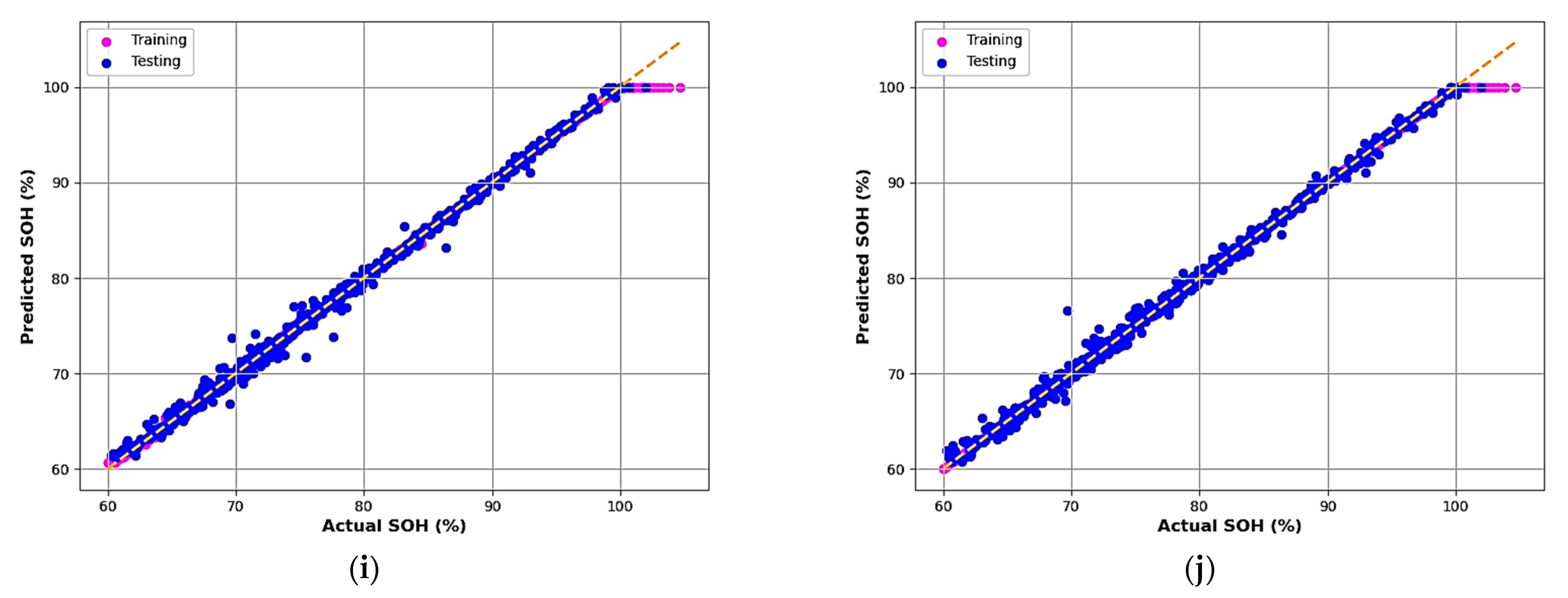
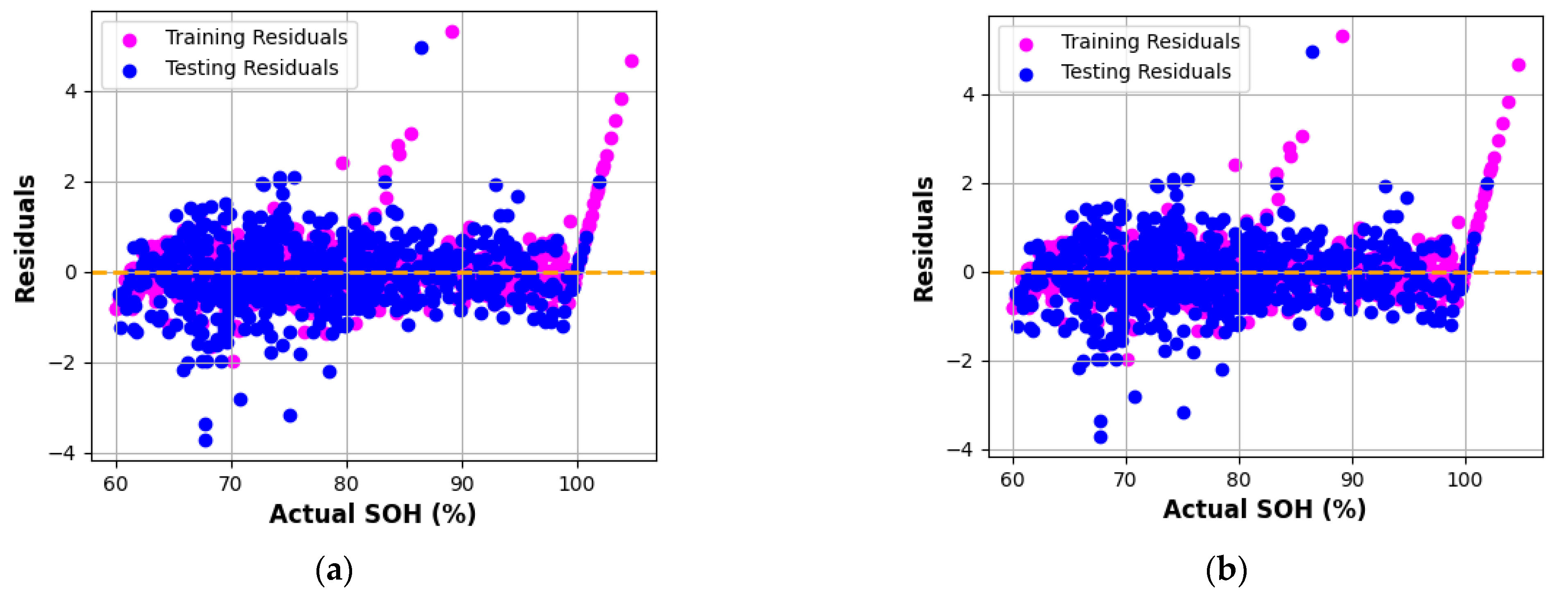
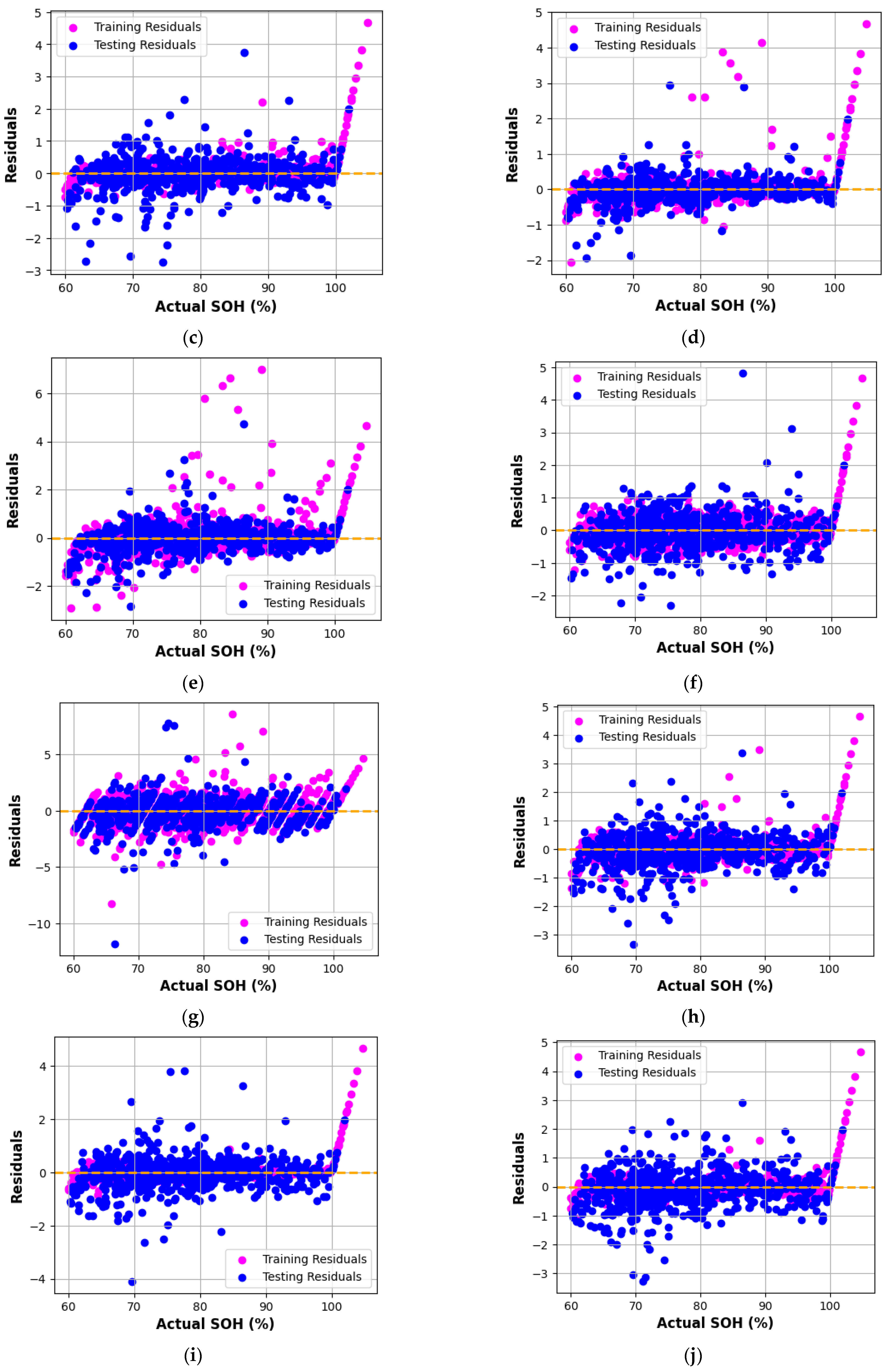
The predictive capability of each algorithm was assessed through multiple graphical diagnostics, including residual and scatter plots, as shown in Figure 3, Figure 4 and Figure 5.

Residual plots (Figure 3) depict the deviation of predicted SOH from experimental values across training and testing data. An ideal model exhibits residuals symmetrically distributed about the zero line, indicating minimal systematic error. Among all the models, Gradient Boosting (GB), AdaBoost (AB), and XGBoost (XGB) display residuals tightly clustered around zero, confirming strong predictive reliability and negligible bias.

Models such as HistGradientBoosting and Random Forest also demonstrate satisfactory performance, though with slightly broader residual dispersion. This minor spread suggests marginally higher variance in prediction errors, likely due to sensitivity to high-frequency EIS components.

The scatter plots in Figure 4 compare the actual versus predicted SOH values for all models. Each subplot shows training (pink) and testing (blue) data points against the 45° reference line (yellow dashed). A close alignment of the points along this line indicates a strong correlation between measured and predicted SOH values. All models exhibit a high degree of linearity, reaffirming the suitability of EIS data for data-driven SOH estimation.

Notably, GB, AB, and XGB models achieved near-perfect regression alignment, with R² ≈ 0.999, MAE ≤ 0.12, and RMSE ≤ 0.28 on training data, highlighting their superior accuracy and consistency.

Figure 5 provides another residual visualization, plotting residuals against actual SOH values. The GB, AB, and XGB models again exhibit compact clustering near zero residuals across the full SOH range (80–100%), confirming their robustness even for highly degraded cells. The Decision Tree and Bagging models, however, show broader residual bands, indicating weaker generalization capability and potential overfitting.

Between the two gradient-boosting variants, GB outperformed XGB by achieving slightly lower error metrics and smoother residual distributions. This can be attributed to GB’s better adaptation to the moderate-sized EIS dataset, whereas XGB tends to excel in larger, more heterogeneous datasets. The limited sample size and high-dimensional impedance features marginally constrained XGB’s convergence precision.

Overall, the Gradient Boosting, AdaBoost, and XGBoost algorithms consistently delivered the most accurate and stable SOH predictions, demonstrating that Bayesian-optimized ensemble learners can effectively capture the nonlinear relationship between impedance spectra and battery degradation.

4.2. Model Explainability and Feature Analysis

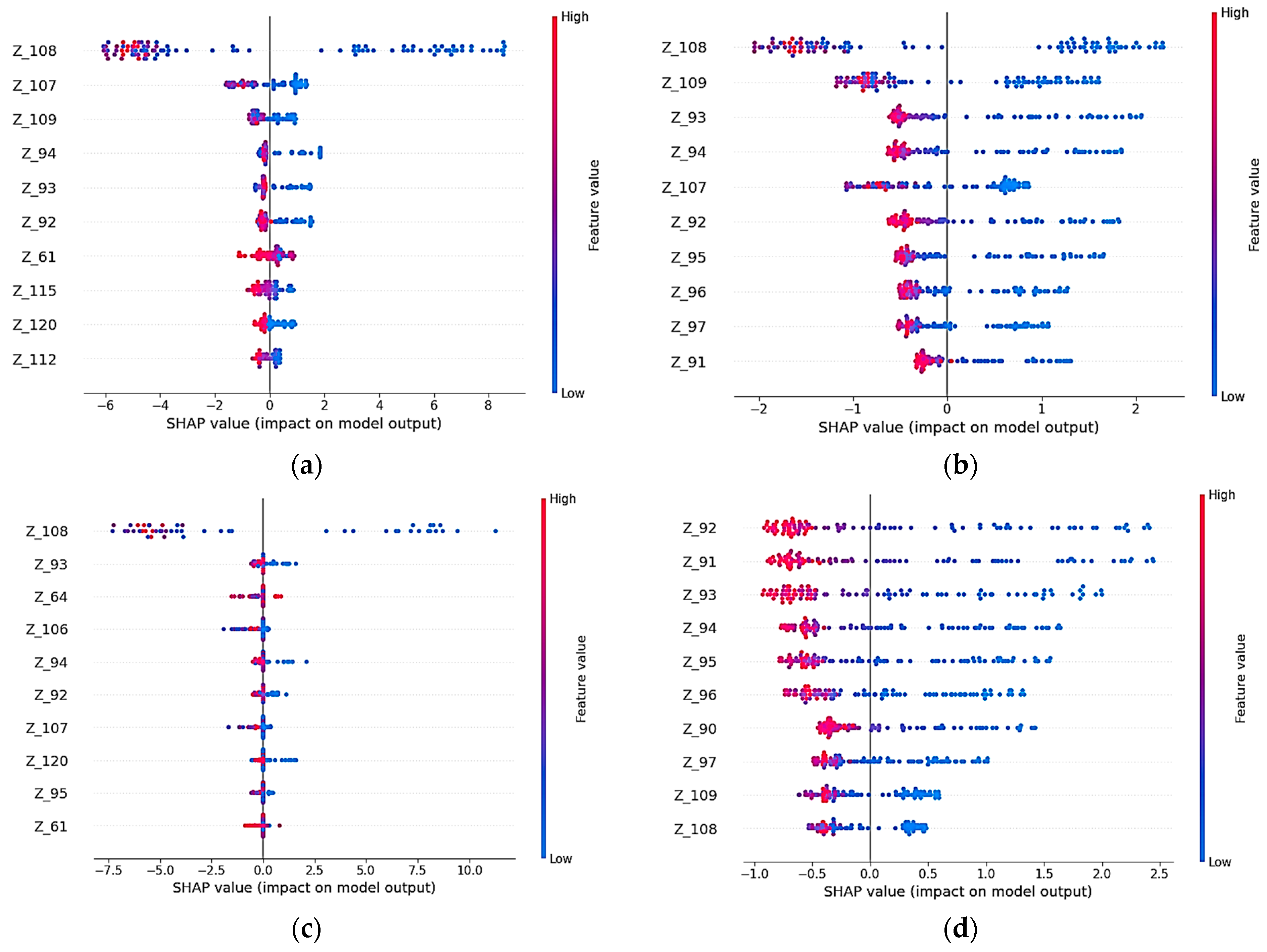
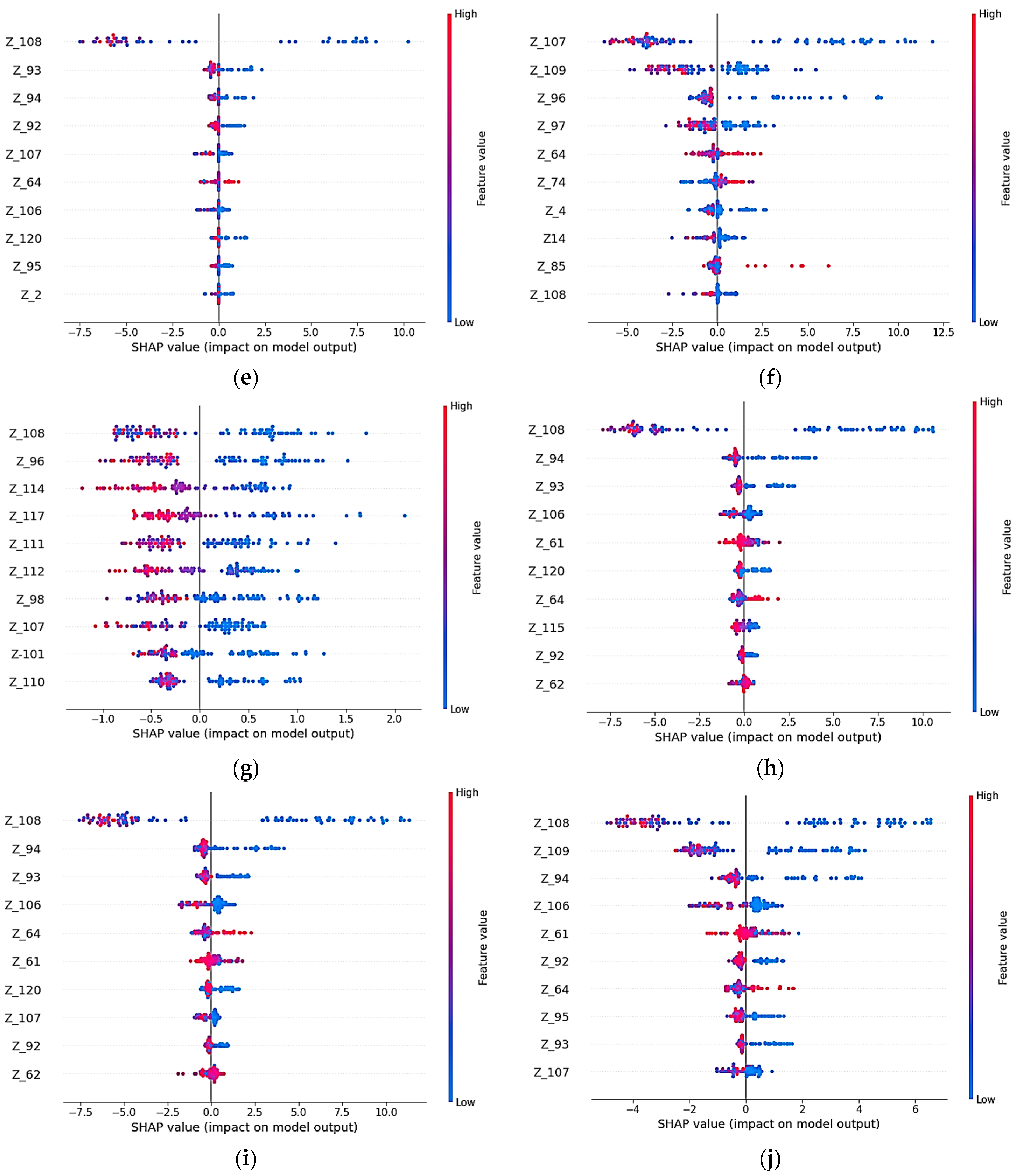
To ensure interpretability, SHAP (SHapley Additive exPlanations) analysis was conducted for all models, as shown in Figure 6. Each subplot reveals how individual EIS features influence SOH predictions. The color gradient from red (high feature value) to blue (low feature value) reflects the directional impact on model output.

Across most models, impedance components Z₁₀₈ and Z₉₄ emerged as the most influential features, showing that specific mid-frequency EIS responses contribute significantly to SOH estimation.

The Extra Trees and CatBoost models uniquely identified Z₉₂ and Z₁₀₇ as key predictors, indicating minor algorithmic variability in how impedance-based relationships are learned. This diversity emphasizes the complementary strengths of ensemble methods in identifying distinct yet physically relevant degradation signatures.

The physical connection between SHAP-identified frequency points and battery degradation mechanisms is established through three major frequency regions. Charge transfer resistance at electrode–electrolyte interfaces, which rises with aging due to SEI layer formation and active material loss, is directly captured by impedance characteristics in the mid-frequency region (30–100 Hz). It is extremely sensitive to capacity deterioration because feature Z94 (imaginary impedance at 57.37 Hz) matches the characteristic time constant of charge transfer reactions (around 2.8 ms). As batteries age, Nyquist plots show this sensitivity through rightward semicircle changes that indicate greater polarization resistance. Physical degradation processes, such as SEI layer evolution and double-layer capacitance variations, are captured by high-frequency measurements at 596.72 Hz and 754.28 Hz (Features Z₁₀₈, Z₁₁₀). Because they react to changes in electrode surface area as well as porosity before major capacity loss occurs, these frequencies are very useful for early degradation detection. Because of its unique impedance signature, the SEI layer, which keeps expanding throughout battery operation, is clearly visible in this frequency band.

Combined ohmic and charge transfer resistance effects are captured by real impedance components (Z₁–Z₆₀). The size of the Nyquist semicircle, which grows systematically with age and is directly correlated with total polarization resistance, is reflected in features at 45 Hz. The bimodal distribution found in SHAP values has a clear electrochemical meaning: the first peak around 57 Hz represents bulk degradation processes (charge transfer, active material loss), while the second peak around 600 Hz implies interface degradation (SEI development, contact resistance). This pattern indicates that battery aging is caused by several concurrent degradation mechanisms that operate at various time constants. Each of these mechanisms leaves unique signatures in particular frequency ranges, which the machine learning model is able to identify as predictive features for the SOH estimate.

By directing the reduced-frequency analysis, these explainability results were incorporated into the suggested protocol: the consistently high-impact features found across models (such as Z₁₀₈, Z₁₀₉, Z₉₄, and Z₁₂₀) fall within mid-to-high frequency ranges. Future potentiostat implementations for BMS applications might prioritize these selected frequency regions rather than performing full 0.02 Hz–20 kHz sweeps, according to this finding, with practical consequences for EIS hardware design. The next generation of fast-scan EIS hardware that is appropriate for embedded battery management systems would be informed by such targeted scanning, which would significantly cut measurement time and expense while maintaining predicted accuracy.

4.3. Comparative Performance Visualization

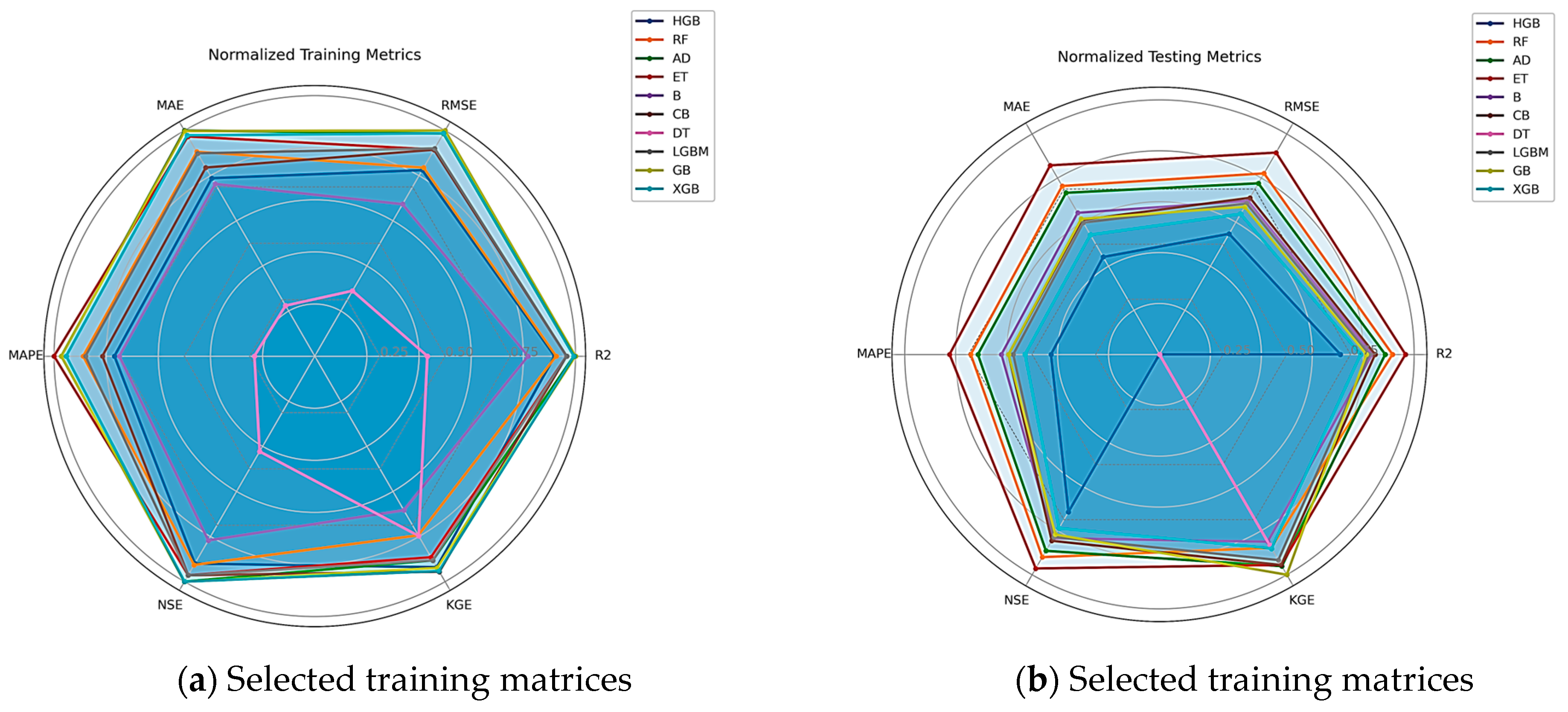
Figure 7 presents radar plots comparing the normalized performance metrics for all models on training and testing datasets.

The larger and more symmetric the polygon, the more balanced the model’s performance across all metrics.

The training results show high accuracy and stability for most models, while testing plots reveal greater differentiation in generalization capability. Gradient Boosting, LightGBM, and CatBoost form the most regular radar shapes, suggesting consistent precision across both datasets.

The radar charts in Figure 7 provide a visual comparison of the performance of each machine-learning model across several standardized evaluation metrics. Models that perform better and more evenly are those that form bigger, more consistent forms. While testing indicates more pronounced disparities in generalization ability, training plots demonstrate that most models attain consistently high accuracy with little variance across metrics.

4.4. Normalized Importance of Factors Under the Model

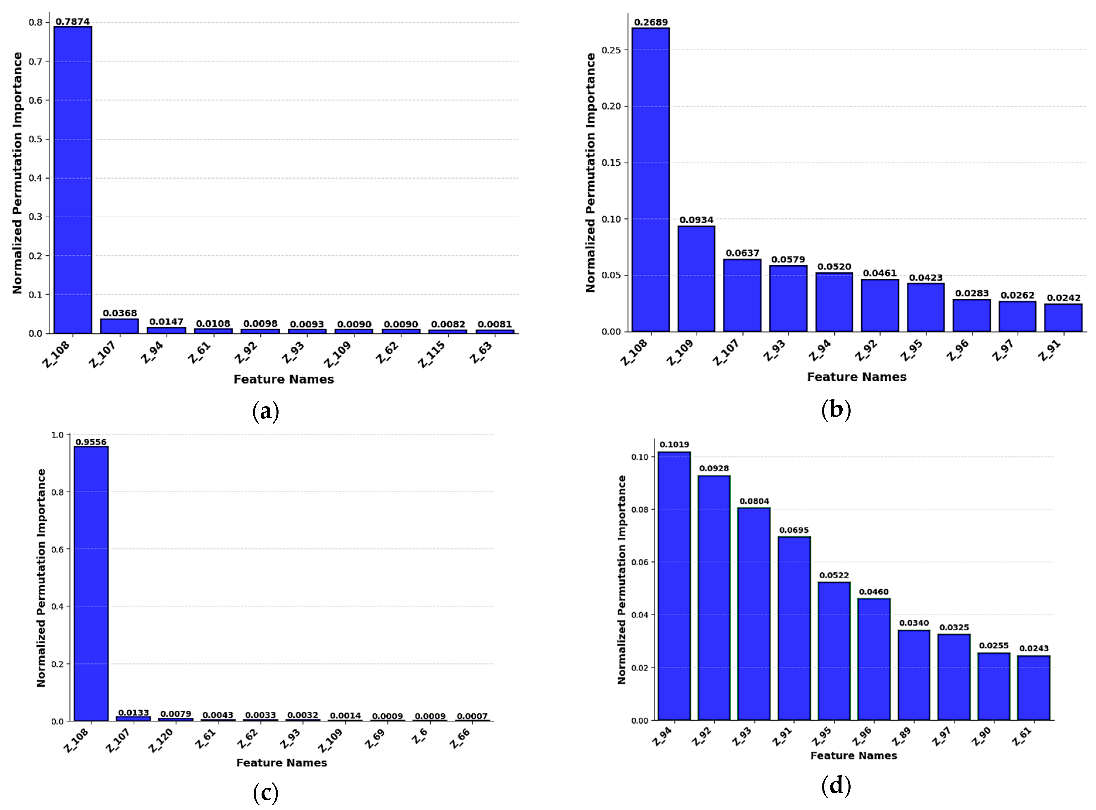
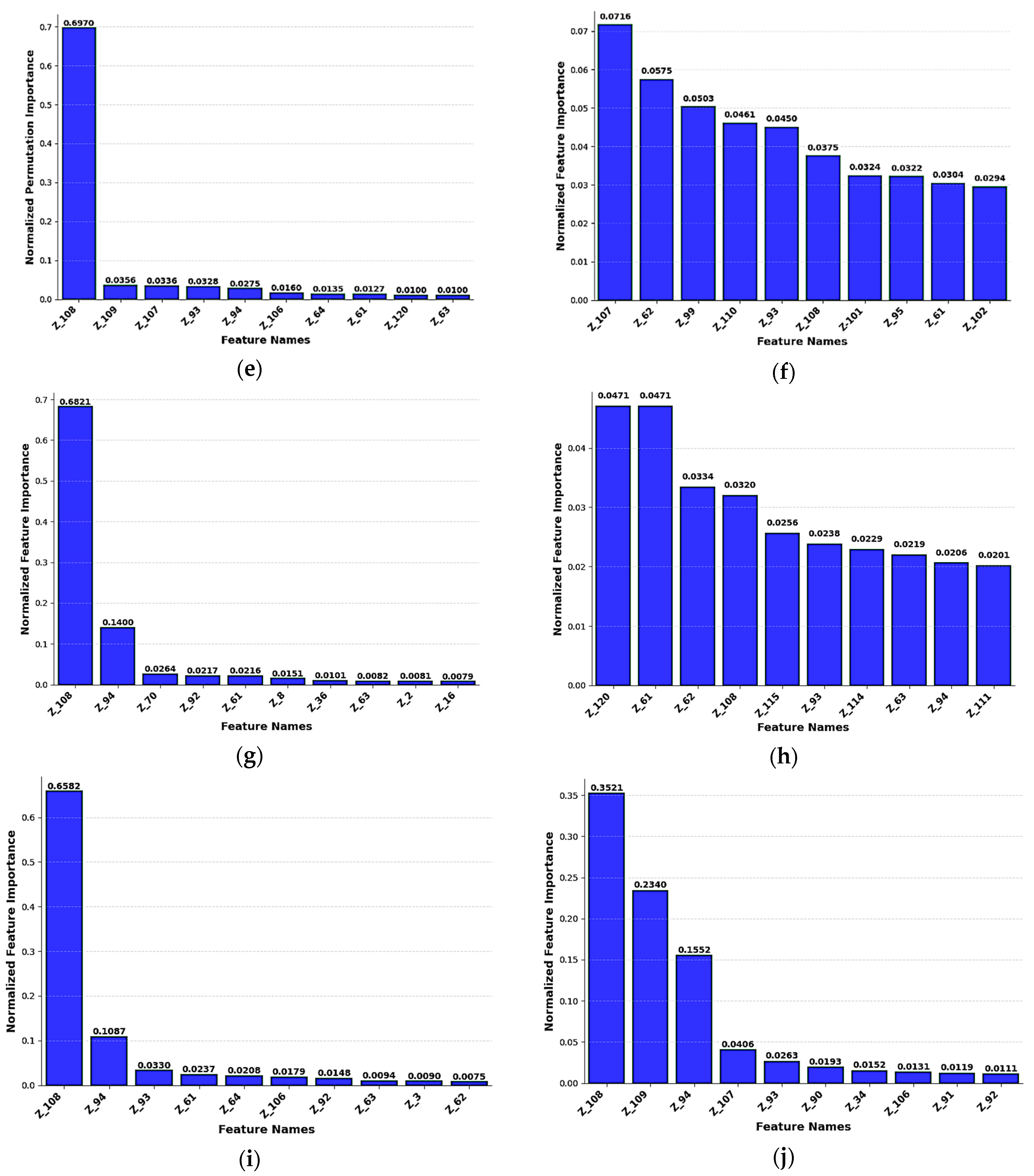
Analysis of ten machine learning models shows significant differences in their use of information for predictions (Figure 8). Bagging shows the highest concentration, with a significance score of 0.9582 for its primary feature, showing a major focus on a single predictor, while other features contribute less than 0.01. AdaBoost has an impressive significance of 0.9136 for its primary feature, showing an essential feature imbalance that could lead to overfitting issues. The Decision Tree and Histogram Gradient models show similar patterns, with their primary features achieving significance scores of 0.7702 and 0.7715. These models indicate the characteristic behavior of tree-based algorithms that automatically identify the most specific elements for split decisions. XGBoost has a feature value of 0.7356, while standard Gradient Boosting shows a feature importance of 0.6441 for its primary predictor.

Random Forest showed superior feature use, with its most significant feature achieving a significance score of 0.2647, showing substantial progress over models that have high levels. The residual features show a more equal distribution ranging from 0.0288 to 0.0623, showing improved feature variety. Extra Trees showed a great stability with an importance score of 0.1619 for its top feature, followed by a slow decline to 0.0394 for the tenth feature. LightGBM provides excellent balance, with its top two features showing similar importance values of 0.0471 and 0.0411, while CatBoost provides the most consistent distribution, with 0.0748 for the primary feature and 0.0429 for the tenth feature.

The analysis clearly shows that CatBoost (Figure 8f), LightGBM (Figure 8h), and Extra Trees (Figure 8d) are superior choices for robust model performance due to their balanced feature utilization, while Bagging, AdaBoost, and Decision Tree models pose significant overfitting risks due to their extreme dependence on single features.

The comparative analysis demonstrates that EIS data, when processed through Bayesian-optimized ensemble algorithms, enables highly accurate SOH forecasting. Gradient Boosting achieved the highest overall accuracy with R² = 0.9996, MAE = 0.104, and RMSE = 0.27 on training data.

The strong agreement between predicted and actual SOH across all high-performing models validates the proposed approach as a practical and explainable diagnostic tool for battery management systems.

The integration of EIS feature analysis and explainable AI ensures not only high predictive accuracy but also physical interpretability—linking impedance characteristics directly to degradation phenomena.

4.5. Overfitting Testing

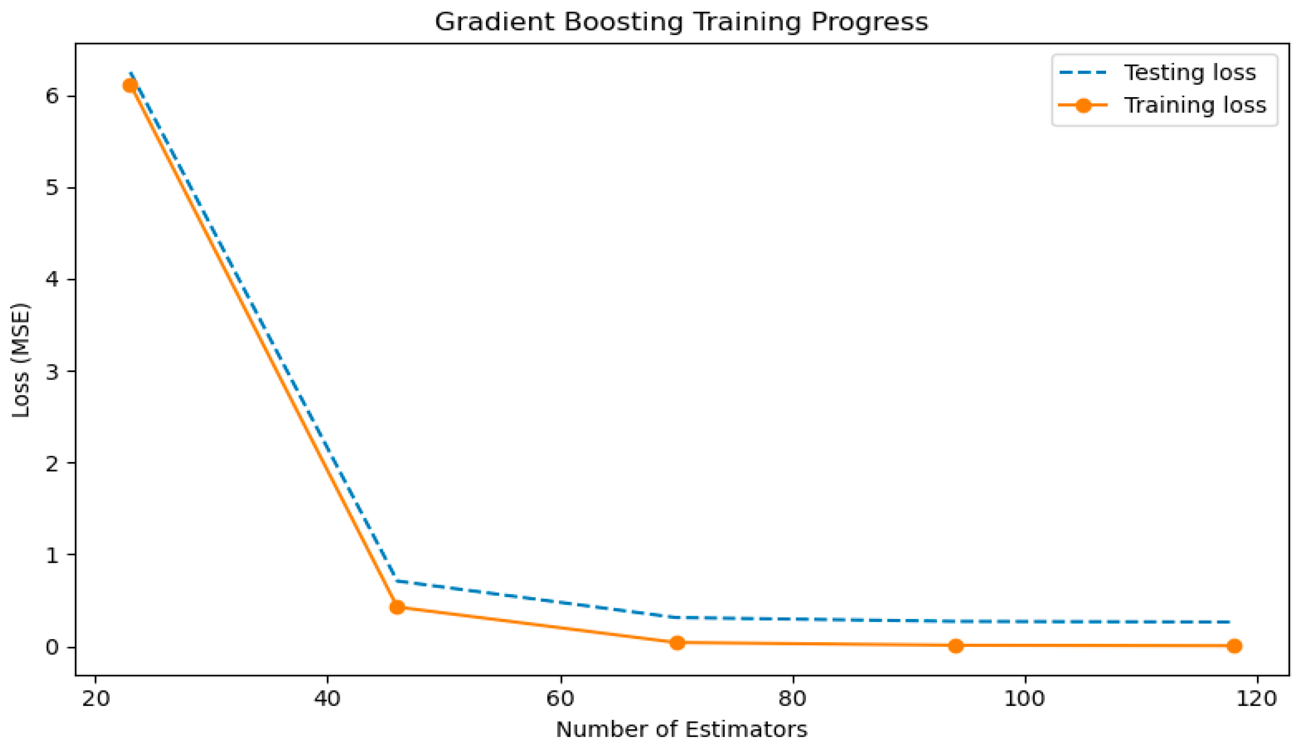
This subsection provides details on overfitting testing of the best-performing model, gradient boosting. Effective model learning is indicated by the learning curve in Figure 9, which shows that both the training and test losses decrease rapidly as the number of estimators increases. There is simply a tiny, steady difference between the two curves since the testing loss closely tracks the training loss throughout. This consistent behavior confirms that the Gradient Boosting model does not exhibit overfitting and generalizes well to unseen data.

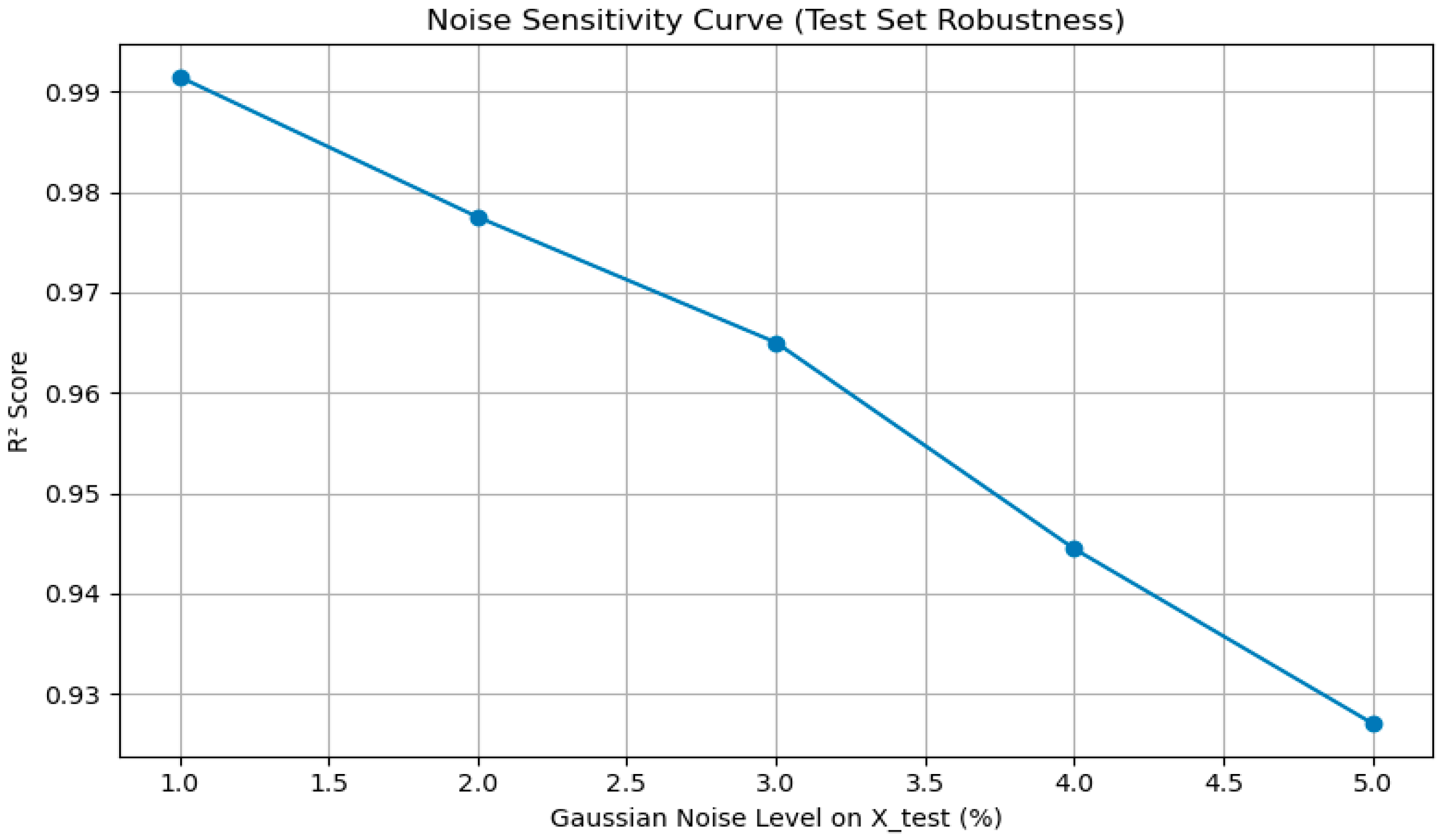
The noise sensitivity curve in Figure 10 shows that the R² score decreases gradually as Gaussian noise increases from 1% to 5%, reflecting the expected impact of measurement perturbations. Despite this added noise, the model maintains high predictive accuracy, with R² remaining close to 0.93 even at the highest noise level. This behavior demonstrates that the gradient boosting model is robust and stable under realistic variations in EIS measurements.

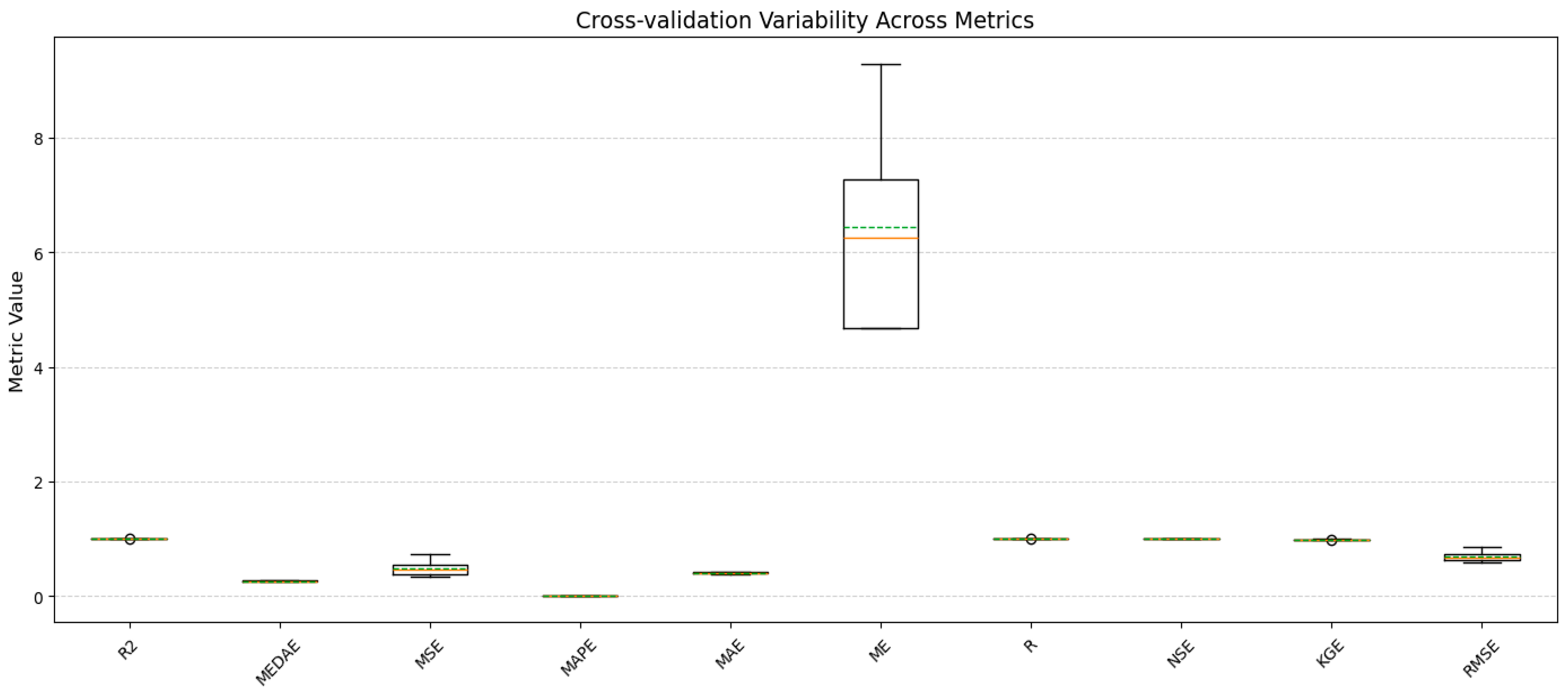
The box plot in Figure 11 illustrates the variability of all evaluation metrics across cross-validation folds for the gradient boosting model. Most metrics exhibit narrow dispersion, indicating stable, consistent performance across data partitions. The wider spread observed for ME is expected due to its signed nature and does not indicate systematic prediction bias.

5. Conclusions

An accurate SOH estimation is imperative to support high-level integration of renewable and EV energy with the systems. This research developed and evaluated ten sophisticated tree-based ensemble models for predicting SOH utilizing electrochemical impedance and operational data. All models demonstrated improved performance through hyperparameter tuning with Bayesian optimization. Gradient Boosting achieved the highest accuracy among all the considered models, with an R² of 0.9996 and minimal MAEs of 0.1044 and 0.4061 on the training and test datasets, respectively. Feature importance analysis indicates that impedance attributes, voltage characteristics, and cycle features are essential for predicting degradation patterns. In summary, the results demonstrate that the proposed optimized ensemble-learning approach enables accurate, comprehensive, and computationally inexpensive estimation of state-of-health. The findings underscore the significance of frequency-focused impedance analysis and explainable AI in facilitating rapid diagnoses, hence enhancing their applicability in practical battery monitoring and intelligent energy systems. In the future, we will validate the proposed framework on larger multi-chemistry datasets, integrate real-time experimental EIS measurements, and extend the methodology to concurrent SOH and residual functional life prediction for practical battery management systems. We also aim to incorporate temperature-compensated features and online learning mechanisms to handle in-field EIS drift, and to assess the cost-effectiveness of combining our approach with established coulomb-counting-based SOH estimation methods.